Inflation Policy and Public Understanding

During the 1970s many argued that government spending, specifically deficits, were a primary, possibly the major, cause of inflation. Ronald Reagan as candidate in 1980 said that he would reduce inflation by balancing the national government budget. The sharp decline in inflation despite a tripling of the deficit during Ronald Reagan's first term, however, suggests that inflation is not simply a result of the national government spending more than it receives in revenues.

Why did inflation fall from 12.4% in 1980 to 3.8% in 1983? Economists from the Urban Institute examined the fall in inflation during the early 1980s and concluded that a number of factors produced lower inflation (Stone and Sawhill 1984, 12–20, especially Table 4, p. 19). They suggested that 1.6 percentage points, 18.6% of the decline, resulted simply from a new measure of inflation, starting in 1983, in which the cost of homeownership was measured differently in the CPI than in previous years. In addition, 2.9 percentage points, 33.7% of the change, resulted from changes in the prices of food and energy, and in the international value of the dollar. Finally, 4.1 percentage points, 47.7% of the change, resulted from “economic slack,” that is high unemployment. Some of these elements can be influenced directly by policy changes but others are only indirectly, if at all, amenable to policy action.

The preferred policies one uses to deal with inflation depend at least partly on one's assumptions about the economy, judgments of causal relationships among various components, and judgments of the ability, tools, and resources of government to address inflation. In addition, ideological orientations—views of what government should do—strongly influence judgments of appropriate economic policy. All this is further complicated in the U.S. context by separation of powers, checks and balances, and the division of economic policy arenas among the president, Congress, the Federal Reserve, and others.

All parties have self-interests in policies directed toward inflation, unemployment, and other economic problems. The gainers and losers from inflation are less clear than those from high unemployment, that is, recessions. The “main relative gainers from recessions are the upper quintiles of the distribution, particularly the highest quintile.”⁴

The primary gainers from inflation, on the other hand, are less clear. Despite the usual view that the poor, those “on fixed incomes,” suffer most from inflation, it appears that inflation, over time, may slightly benefit those low in the income scale though the effects are small and not totally clear (Hibbs 1987, Ch. 3, especially p. 77–89).

Reflecting a combination of self-interest and ideology, identifiers with the two political parties diverge in their orientations toward the relative importance of inflation and unemployment as policy goals. Republicans generally emphasize low inflation as a primary goal while Democrats emphasize low unemployment (Hibbs 1987, Ch. 1–4).

Clarifying Terms: Inflation, the Consumer Price Index (CPI), and Cost of Living

The U.S. Bureau of Labor Statistics (BLS) has collected systematic data about prices since 1913, making CPI data available beginning that year. Economic historians, the BLS, and other organizations and individuals have estimated price levels for earlier years; Historical Statistics of the United States, last fully updated in 1975, presents price level estimates starting 1800. More recently, economic historians have revised and updated those earlier estimates and have produced price level estimates starting with 1665 (see McCusker 2001; the data he presents will be used in later editions of Historical Statistics). Although very large social, economic, and political changes have occurred since 1665, those estimates present at least a rough approximation of price levels and changes during a long period of American history. This paper uses those data—“re-based” so that 2003 is the base year, that is, equal to 1.000 or 100—to present U.S. historical data about politically relevant topics that involve dollar figures.

It is important to recognize that the CPI has strengths and limits. Although the CPI often is referred to as a “cost of living” index, in reality it more accurately can be described as a “cost of goods” index because it is based on changes in the prices of a “fixed market basket” of goods (Schultze and Mackie 2002, Executive Summary and especially ch. 1). The CPI (usually the CPI-U, for urban consumers, rather than the narrower CPI-W, for workers, which represents a smaller part of the U.S. public) is based on a “market-basket” of goods and services with many components and weightings to approximate purchasing patterns of U.S. households. The BLS and Census Bureau regularly sample the prices of the items in the market basket and use those prices to produce the CPI. The market basket, of course, changes over time, and a potential weakness of the CPI is that over time the components and weightings in the market basket diverge increasingly from actual purchasing patterns until adjustments occur. In addition, economists have long recognized that quality improvements may not be reflected directly in prices and so in the CPI, as illustrated by falling prices but rising quality for computers.

For these and a variety of other reasons, the CPI is changed periodically, with small revisions occurring periodically. The most recent major revision occurred starting in 1983, when a new measure of housing costs was introduced. Economists had long thought that the former CPI exaggerated the effect of changes in housing prices, so the post-1982 measure corrects for that. (As noted earlier, Urban Institute economists have estimated that 18.6% of the total reduction in inflation from 1980 to 1983 was due to this change in the CPI measure.) To provide historical continuity, the BLS and Census Bureau also calculated what price levels from 1950 to 1982 would have been using the new measure; that series is called CPI-U-X1. The BLS, the Census Bureau, and several other government agencies have developed various experimental measures of inflation.⁵

Much confusion accompanies measures of inflation on the part of officials and especially among the public. Because the inflation “market basket” attempts to reflect an average market basket of purchases, to some degree it does reflect cost of living. However it does not directly measure “standard of living,” which reflects changes in income and other measures of resources relative to changes in price levels.

One effect of this distinction is that low inflation is not necessarily associated with increases in standard of living. For example, if prices rise an average of 10% but wages rise an average of 12%, a net increase in average purchasing power occurs. If inflation falls to, say, 4%, but wage increases fall even more, say to 2%, a net decrease in purchasing power occurs.

An important set of limits in relation to inflation measures is that both price changes and income data are averages, and there is much variation in both. The various elements of the “market basket” on which the CPI is calculated often rise at different rates.⁶

Because the CPI represents an average, probably no specific individual's personal “market basket” exactly matches that of the CPI. As a result, those who purchase items whose prices rise less than overall price changes may experience a different effect on standard of living than implied by CPI changes. Similarly, there is large variation in income changes, so that some individuals experience income changes that offset price-level changes while others do not.

It also is important to recognize that living standards are affected not only by price changes but also by improvements in quality and other changes in various components of items purchased and by emergence of new items that improve standard of living. CPI, as noted, is changed periodically to reflect new items, improvements in quality, and so on, but the changes might not perfectly reflect the product changes and involve a lag in reflecting items in the CPI.

Probably a better measure of changes in standard of living is to denominate items purchased not only in inflation-adjusted dollars but also in terms of “work-hours,” “work-days,” or similar. For example, the income from the work of how many minutes, hours, or days was needed to purchase such items as specific types of food, or an automobile, or a long-distance telephone call in, say, 1950 and 2000?⁷

Even this, of course, does not reflect changes in preferences over time, the emergence of new products (say, cell phones or VCRs), or the fact that new inventions available only to the wealthy (e.g., the automobile, the PC) eventually become necessities.

Data limits and public views affect the ability to examine many potential comparisons over time. Price data for particular items are spotty over long time periods, and particularly there are limits on earnings data prior to the 1940s. However, some economists have examined family budget and similar data over long periods of time and economic historians have developed estimates of the pay of various parts of the workforce.⁸

Still, public views of inflation may be confused not only by incomplete understanding of inflation measures but also by daily experience. For example, the prices of some relatively small items that are purchased regularly tend to rise in increments that may be relatively steep, for example, the rise in price for pay phones calls from 25 to 35 to 50 cents over a short time period. These increases may lead to public judgments of inflation that differ sharply from the official measures of price changes.⁹

Using Inflation Measures to Examine Politically Relevant Topics

Many elements of political history involve dollar figures over time, yet news accounts and even scholarly analyses often do not take into account the effects of changes in price levels. Because inflation adjustment may reveal trends that are not evident using “current” (that is, non-inflation-adjusted) dollars, this paper shows historical trends of selected politically relevant topics taking into account changes in price levels, that is, inflation or deflation.

The web site http://www.orst.edu/ Dept/pol_sci/fac/sahr/sahr.htm includes the data presented here and many other examples. It also provides links to other sources of information about inflation and related topics and provides tables of “conversion factors” which can be used to convert dollars of any year from 1665 to dollars of recent years. Inflation estimates for this year are used to produce conversion factors to dollars of this year, but because these are only estimates this paper uses 2003 conversion factors based on final 2003 CPI.

The data used to produce the conversion factors were collected by many organizations using various methods, some of which have changed over time. Generally, estimates for the distant past—for example, spending in the 1860 presidential election campaign, or price levels in the late 1600s—are less complete and accurate than for more recent time periods.

The following graphs show data in constant (inflation-adjusted, or real) dollars. Some graphs also present data in current dollars (that is, non-inflation-adjusted).

What follows, then, must be read with the recognition that seemingly precise measures have numerous limits, so changes must not be taken too literally. Nevertheless, examining politically relevant data over time using inflation-adjusted dollars often shows striking, and sometimes surprising, patterns.

The Size of the US Economy through U.S. History, Overall Price Levels, and Price Level Changes (Inflation or Deflation)

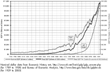
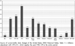
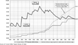
Graph A shows the size of the American economy (Gross Domestic Product, GDP) for the period 1789 to 2003 in billions of inflation-adjusted (2003) dollars. (The current-dollar data are from Economic History Net, at http://www.eh.net/hmit/gdp/gdp_answer.php.) It also shows GDP per capita in inflation-adjusted dollars. (Reliable GDP data are available starting 1930; economic historians have estimated GDP for earlier years.)

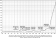
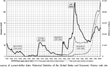
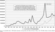
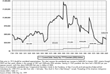
Graph B shows price levels and estimates for the period 1665 to 2014. (Estimates for 2004 to 2009 are averages of estimates by the Office of Management and Budget and the Congressional Budget Office; after 2009, only CBO.) As the graph shows, the U.S. price level in 1945 was essentially the same as price levels at several earlier peaks: the War of 1812, the Civil War, and the early 1920s. The graph also shows that price level changes involve both increases (inflation) and decreases (deflation). Deflation has not occurred since the 1930s in the United States, though it has occurred in Japan and some fear its reemergence in the U.S.

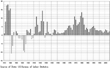
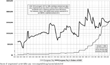
Graph C shows price level changes (inflation or deflation) year-by-year for the period 1915 to 2003. The chart shows the deflation associated with the Great Depression and the high inflation associated with wars and during much of the period beginning in the late 1960s.

Levels of National Government Spending and the National Debt

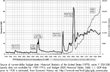
Examining national government budget trends using dollars adjusted for inflation often shows counter-intuitive results. That is, national government spending and the national debt adjusted for inflation show quite different trends than when presented in “current” dollars. Similarly, spending changes during presidential terms also show quite sharp differences when price level changes are accounted for. Graph D shows national government outlays (spending in a particular fiscal year) from 1792 to estimated 2004, in inflation-adjusted (2003) dollars. (Yearly data are not available for 1789–1791.) It also shows national government spending relative to the size of the economy (GDP; reliable data of which began in 1930).

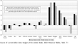
Graph E shows change in inflation-adjusted national government spending (outlays) by presidential term, from 1952 to estimated 2004 calculated from current-dollar data in Bush administration budget documents for fiscal year 2005, in early 2004. (This graph uses CPI-U-X1, which applies the same CPI measure to the entire period starting from 1950. All graphs here that involve only the period starting from 1950 use the CPI-U-X1.)

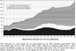
Graph F shows U.S. national debt (accumulated deficits) from 1792 to estimated 2004 in three ways: current dollars, constant (2003) dollars, and as percent of GDP. Graph G shows changes in inflation-adjusted national debt by presidential term for Presidents Truman to estimated George W. Bush. As noted on that graph, the broader measure “gross debt” generally is considered less important economically than “debt held by the public,” which excludes debt held by the Social Security trust funds and similar national government units. (For comparability over the entire time period, Graph F shows total or gross national debt rather than separately showing debt owned by the public.)

The Composition of National Government Spending

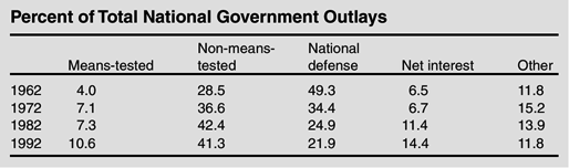
The composition of the national government budget has changed sharply during the second half of the twentieth century. The table shows that as percent of total outlays the share for both means-tested and non-means-tested programs has increased and the share for national defense spending has decreased.

The table shows four major categories of national government spending—defense, net interest, means-tested social spending, and non-means-tested social spending—and a residual “other” category for the period starting 1962. (The 1962 budget year is the first for which consistent data for these spending categories, from the Congressional Budget Office, are available.) The largest nonmeanstested programs are Social Security and Medicare. The largest meanstested program is Medicaid. Graph H shows outlays in constant (2003) dollars for each of those categories for the period 1962 to estimated 2004.

Graph I enlarges on long-term trends for the largest federal-funds item of the national government budget, national defense. Although defense has fallen during recent decades as percent of outlays and of the economy, from the 1950s through the 1970s it stayed within the relatively narrow band of $250 to $300 billion in dollars of 2003, except for increases during the Vietnam War. Since the buildup in defense spending under President Reagan, defense spending fell to a low point of slightly below $300 billion before rising during the late Clinton presidency and increasing even more during the George W. Bush presidency.

Although national defense spending has fallen as percent of total national government spending, it has remained in recent years at about half of total national government discretionary spending, the part “controllable” by Congress and the president through the appropriations process. At the same time defense spending fell as percent of total spending, discretionary spending share of total spending also fell sharply, from 67.5% in 1962 to 43.7% in 1982, and to 36.5% in 2002.

A major reason defense spending has such large impact on presidential and congressional budgetary decisions is that it is by far the largest single category of discretionary spending. In budget year 2002 defense was 47.5% of discretionary spending; it is a larger share more recently and in the near future. Defense is not only a very large share of discretionary spending but it vastly dwarfs all the other discretionary spending items. Defense was $348.9 billion in budget year 2002 and the second largest discretionary category, education, was a very distant second, about one-eighth as large, at $43.3 billion or 5.9% of discretionary spending. Because defense spending is increasing and other growth in other discretionary spending is slowing (or in some instances decreasing in real dollars), defense spending soon will rise to more than half of discretionary spending.

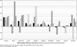
Governor and presidential candidate George W. Bush in 2000 stated that when examining changes in state, and presumably national, government spending, both inflation and population change should be taken into account. Graph J shows change in inflation-adjusted outlays per-person by presidential term for overall spending and for each of the earlier categories, from President Johnson through President George W. Bush. This graph shows change, using Census Bureau population data, to control not only for price changes but also population changes.

Graph J challenges a number of elements of “conventional wisdom” (CW) about spending by Republican and Democratic presidents, for example that Democratic presidents increase and Republican presidents decrease social spending and that Republican presidents increase and Democratic presidents decrease defense spending. That graph instead emphasizes that changes in domestic spending are related to policy changes somewhat independent of presidential party. For example, large increases in social spending occurred under Republican President Nixon as Social Security and other policies were changed. Similarly, defense spending levels are related more to historical circumstances—the beginning and ending of wars, for example—and less to the party of the president. For example, until the current Bush presidency, the only Republican president since Dwight Eisenhower to increase defense spending was Ronald Reagan. Increases during his terms may have been the most important factor in establishing the CW about presidential parties and defense spending.

Social insurance programs in the United States are much more widely supported than public assistance programs. This difference is reflected in changes in inflation-adjusted benefit levels for programs in each category. Prior to 1974, Social Security benefit levels were changed by congressional and presidential action, often resulting in large increases in “even numbered” (election) years. Legislation in 1974 produced automatic adjustment of Social Security benefits starting in 1976. Welfare programs, on the other hand, are not adjusted automatically to offset price level changes. Notice that in 1970 the benefit levels of the two programs were relatively close but since that time there has been large divergence. Graph K shows inflation-adjusted benefit levels for Social Security and “welfare” (first AFDC, later TANF) for the period starting 1936 (data are not available for both series for all years). The dollar values of each are indicated for 1970 and 2000 to illustrate divergent trends in benefit levels.

Similarly, the minimum wage has been a subject of political conflict since its establishment in 1938. During long periods it has fallen in inflation-adjusted dollars. Graph L shows inflation-adjusted minimum wage for each year from its origination in 1938, indicating its peak in the late 1960s and its decline during long periods. The graph also shows what its current-dollar value would have had to be in various years to equal the peak level (1968) in inflation-adjusted value.

Campaign Spending and Campaign Contribution Limits

Surprising trends appear when examining campaign spending. The quality and completeness of data, especially for the earlier periods, almost certainly vary. So, as with some of the other data presented here, the underlying data almost certainly are not complete or precisely comparable for the entire period. Graph M shows spending for presidential general election campaigns from 1860 to 2000.

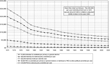
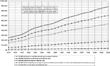
Contribution limits have been a central element of recent campaign finance issues. The following two graphs show the limits established in 1974 in two ways: First, Graph N shows the value in dollars of 2003 of the 1974 spending limits for each year starting 1974. Second, Graph O shows what the 1974 contribution limits would have had to be each year to maintain the same purchasing power as 1974. These data provide ammunition for those who argue that, at the least, campaign contribution limits should be increased given their sharp decrease in purchasing power since the 1970s.¹⁰

Most people appear to believe that the pay of government officials always increases. Yet for both presidents and members of Congress, pay in recent years is less, adjusted for inflation, than in many earlier years. For example, Graph P shows presidential pay from George Washington to President 2004. As that indicates, President Clinton's $200,000 yearly pay made him, in inflation-adjusted dollars, the lowest paid president in American history, with an average in 2003 dollars of $230,000 during his two terms. When yearly presidential pay had been increased from $100,000 to $200,000 in 1969, that equaled about $3005,000 2003 dollars; it had fallen to about $214,000 2003 dollars in Clinton's last year, before rising to $400,000 ($415,000 2003 dollars) with the inauguration of the new president. William Howard Taft's $75,000 per year, the equivalent of about $1,400,000 2003 dollars, made him by far the highest paid. And the pay of members of Congress, $158,100 in 2004, reached a peak, adjusted for inflation, in 1969, at about $214,000 in dollars of 2003, as Graph Q shows.

The pay of both presidents and members of Congress have declined sharply since 1960 relative to the pay of corporate officials. In 1960, the pay of top-500 CEOs, using Business Week data, was 1.9 times that of the president and 8.5 times that of members of Congress; in 1970 the ratios were 2.7 and 24.4, respectively, in 1980, 3.1 and 14.7 respectively, and in 1992 17.5 and 27.0, respectively. During the 1990s the ratios zoomed upward, to 28.9 and 43.3 in 1996 and to 65.5 and 92.7 in 2000, before declining the past two years.

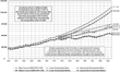
In addition, trends in family income in inflation-adjusted dollars suggest that if 1947 to 1973 average growth in inflation-adjusted family income had continued after that time, the median family income in 2001 would have been about $110,000 (assuming exponential growth best fit), nearly twice as high as the actual median (linear growth would have produced a median of 70–75,000), as Graph R shows. That faster rising family income during the post-1973 period would have had very large political effects.

Trends in many other politically relevant topics show surprising results when examined using inflation-adjusted dollars. (All those shown here, and many others, are shown on the web site indicated earlier.)

All these data, using inflation-adjusted dollars, help illuminate trends in American politics that are less clear if non-inflation-adjusted dollars are used. Many of these also challenge “conventional wisdom” about such topics as presidents, the size of government, and other elements. And, at the least, they emphasize the importance for careful political analysis of adjusting dollar figures over time for the effects of price changes.