1. Introduction
Though buoyancy forces in Rayleigh–Bénard (RB) convection act only vertically, pressure drives horizontal motion as well. For some geometries and boundary conditions, mean horizontal motion can arise that is stronger than the vertical motion by several orders of magnitude. Here we simulate RB convection in a two-dimensional layer with periodicity imposed in the horizontal direction, focusing on states with horizontal mean flow at moderate-to-large Rayleigh numbers. Such mean flows are vertically sheared, and this large-scale shear alters many bulk properties of the convection by shearing all smaller flow structures in the same way. Hence, we refer to such states as shearing convection. States without mean shear, which might be thought of as ordinary RB convection, we refer to as non-shearing convection. By analogy with wavenumber-zero mean flows in planetary atmospheres and tokamak plasmas (Diamond et al. Reference Diamond, Itoh, Itoh and Hahm2005), which are discussed below, we refer to the mean horizontal flow as zonal flow. Both zonal flow and non-zonal flow are present in shearing convection, whereas the zonal component either is absent from non-shearing convection or vanishes in long-time averages.
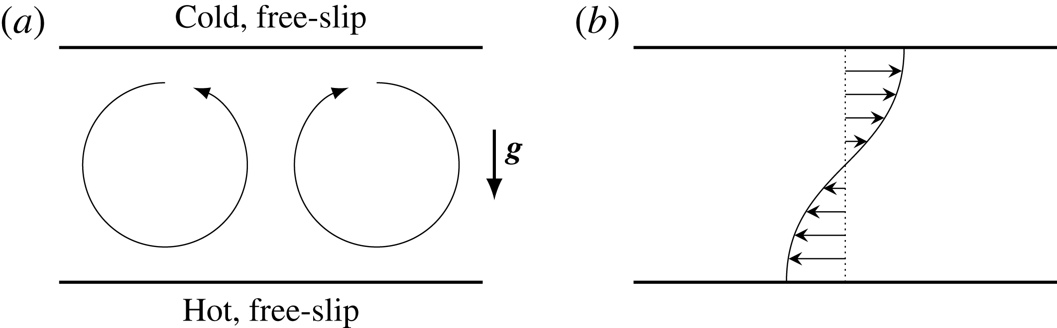
Our configuration is shown in figure 1, which includes schematics of the vortical motions that typically drive two-dimensional (2D) convection and the sort of mean zonal flow profile that can arise. Free-slip conditions are imposed at the top and bottom boundaries. This configuration, perhaps more than any other, encourages very strong mean flows: horizontal periodicity allows for mean flow with a horizontal wavenumber of zero, free-slip boundaries apply no shear stresses to slow the fluid, and two-dimensionality precludes transverse perturbations that can disrupt the mean flow. The zonal flow will always be vertically sheared since conservation of horizontal momentum requires any mean flow developing from static fluid to consist of both left-going and right-going regions, as in figure 1(b). Our chosen geometry is the simplest finite domain in which convection can drive wavenumber-zero mean flow. Other examples, all of which must have a periodic coordinate, include azimuthal mean flow in an annulus and longitudinal mean flow in a spherical shell.
The configuration of 2D RB convection studied here with schematic drawings of (a) the vortical motions typical of 2D convection and (b) the sort of mean zonal flow that can develop with free-slip boundary conditions. The downward direction of gravity (
 $\boldsymbol{g}$
) is indicated.

The shearing convection we study here differs in several ways from the ordinary (non-shearing) RB convection described, for example, in the review of Ahlers, Grossmann & Lohse (Reference Ahlers, Grossmann and Lohse2009). Because zonal flow helps disperse thermal plumes (Terry Reference Terry2000), it can significantly depress the net heat transport, along with the accompanying work expended by buoyancy, thereby inhibiting its own source of energy. These trends are qualitatively understood, but quantitative questions remain. In particular, for what parameters can shearing convection persist? And, when it does, how energetic will the zonal flow be, and how quickly will heat be transported?
Past studies of shearing convection have been motivated either by experimental or planetary convection or by plasmas in tokamaks. These applications share several features with our RB model. First, at least one boundary is often modelled as free-slip in the study of both atmospheres and tokamaks. Second, the zonal flows that form are sheared normally to their directions of motion and inhibit transport in these normal direction. Finally, anisotropies render fluid motion roughly two-dimensional locally. This is achieved in tokamaks by fast equilibration along magnetic field lines (Wesson Reference Wesson2011) and in rotating atmospheres by the Taylor–Proudman effect.
In horizontally isotropic three-dimensional (3D) domains, persistent shearing convection has not been reported, nor have we found it in our own preliminary simulations. It thus appears that simulating shearing convection requires adding an anisotropic effect to 3D convection or, as in this work, imposing two-dimensionality. (The need for anisotropy in 3D is supported by the asymptotic analysis of Massaguer, Spiegel & Zahn Reference Massaguer, Spiegel and Zahn1992 and by the transient nature of zonal flow in the reduced model of Matthews et al. Reference Matthews, Rucklidge, Weiss and Proctor1996.) Zonal flow can arise also in systems driven by means other than buoyancy (Drake et al. Reference Drake, Finn, Guzdar, Shapiro, Shevchenko, Waelbroeck, Hassam, Liu and Sagdeev1992; Finn, Drake & Guzdar Reference Finn, Drake and Guzdar1992; Childress Reference Childress2000), but only with buoyancy can the zonal flow inhibit the very convective structures that drive it – an important feedback found in applications like planetary atmospheres and tokamaks.
In laboratory convection experiments, large-scale mean flows in domains of large horizontal extent have been described by Malkus (Reference Malkus1954a ) and Krishnamurti & Howard (Reference Krishnamurti and Howard1981). In rectangular and cylindrical domains with horizontal extents comparable to their heights, weaker mean ‘winds’ that may drift or reverse direction are often seen in physical and numerical experiments (Ahlers et al. Reference Ahlers, Grossmann and Lohse2009). It is possible that finite-wavenumber circulation will resemble zonal flow more and more as the domain is widened. If so, periodic domains offer a way of studying this limit without the computational expense of simulating very wide domains. In either case, the zonal flow we study here is distinguished from the better known winds by its greater strength, its permanence once established, and its ability to significantly depress vertical heat flux.
Planetary atmospheres derive much of their kinetic energy from buoyancy forces, and it has been suggested that the upscale kinetic energy transfer that drives zonal flow in RB convection also drives atmospheric zonal jets (Thompson Reference Thompson1970; Busse Reference Busse1994), in concert with other mechanisms (e.g. Scott & Polvani Reference Scott and Polvani2007). Simulations with rotation have produced zonal flow in 2D domains like our own (Brummell & Hart Reference Brummell and Hart1993), in annuli (Morin & Dormy Reference Morin and Dormy2004; Tao & Tan Reference Tao and Tan2010; Calkins et al. Reference Calkins, Aurnou, Eldredge and Julien2012; Teed, Jones & Hollerbach Reference Teed, Jones and Hollerbach2012), and in 2D spherical shells modelling stars (Ballot, Brun & Turck-Chièze Reference Ballot, Brun and Turck-Chièze2007; Brown et al. Reference Brown, Browning, Brun, Miesch and Toomre2008) and gas giants (Christensen Reference Christensen2002; Heimpel & Aurnou Reference Heimpel and Aurnou2007; Kaspi, Flierl & Showman Reference Kaspi, Flierl and Showman2009; Heimpel & Aurnou Reference Heimpel and Aurnou2012). Many of these simulations also display the sort of pronounced bursts that we describe here without rotation.
In toroidal tokamak devices, zonal flows in the poloidal direction are crucial to the effort to confine plasmas magnetically. This has motivated studies of models similar to the present one, as reviewed by Garcia et al. (Reference Garcia, Bian, Naulin, Nielsen and Rasmussen2006), even though some important effects are lost in 2D. If a tokamak plasma is regarded as a magnetohydrodynamic fluid, the radial ‘interchange motions’ driven by centrifugal forces are analogous to RB convective motions. Interchange motions harm plasma confinement by adding to radial transport, but they can also drive poloidal zonal flow that lessens this harm, much as RB convection can drive horizontal zonal flow that reduces vertical heat flux. In plasma terminology, the onset of zonal flow is credited with the transition from the low-confinement mode to the high-confinement mode that has been seen in many devices and is considered essential for achieving fusion (Terry Reference Terry2000; Diamond et al. Reference Diamond, Itoh, Itoh and Hahm2005; Wagner Reference Wagner2007). Here, we use the Nusselt number to quantify the depression of heat transport by zonal flow. Plasma physicists might prefer to think of this depression as an increase in confinement.
Among past work on horizontally periodic 2D convection, shearing convection is absent from most analytical studies, perhaps because it does not occur in the weakly nonlinear regime for generic parameter values (Howard & Krishnamurti Reference Howard and Krishnamurti1986; Rucklidge & Matthews Reference Rucklidge and Matthews1996; Goluskin Reference Goluskin2013). Instead, shearing convection has been found using direct numerical simulation (Thompson Reference Thompson1970; Finn Reference Finn1993; Bian et al. Reference Bian, Benkadda, Garcia, Paulsen and Garbet2003; Garcia & Bian Reference Garcia and Bian2003; Garcia et al. Reference Garcia, Bian, Paulsen, Benkadda and Rypdal2003; Zhu & Flierl Reference Zhu and Flierl2012; van der Poel et al. Reference van der Poel, Ostilla-Mónico, Verzicco and Lohse2014), numerical bifurcation analysis (Rucklidge & Matthews Reference Rucklidge and Matthews1996), and reduced models (beginning with Howard & Krishnamurti Reference Howard and Krishnamurti1986). Still, parameter space has scarcely been explored at large Rayleigh numbers, despite the fact that plasma-physical and astrophysical applications fall in this regime. The tokamak-motivated simulations by Garcia, Bian, and collaborators give some tantalizing first results: when zonal flow is present at a Prandtl number of unity, convective transport occurs in bursts and is, on average, significantly lessened. We expand on these findings here, computing integral quantities in a larger spatial domain and over greater ranges of the control parameters.
The governing equations are introduced in § 2. The shearing convection we simulate can be roughly divided into two categories. At larger Prandtl numbers, the convective transport is strong at all times, so we say that the shearing convection is sustained. At smaller Prandtl numbers, convective transport comes in pronounced bursts, so we say that the shearing convection is bursting. Sustained and bursting flows are described in § 3 and § 4, respectively. Heat transport in both sorts of shearing convection is summarized in § 5. Discussion is offered throughout, and concluding remarks appear in § 6.
2. Governing equations
We adopt the Boussinesq approximation, in which the fluid has constant kinematic viscosity,
 ${\it\nu}$
, and thermal diffusivity,
 ${\it\kappa}$
. We non-dimensionalize lengths by the layer height,
 $d$
, times by the thermal diffusion timescale,
 $d^{2}/{\it\kappa}$
, and temperatures by the decrease,
 ${\it\Delta}$
, from the bottom boundary to the top one in the static state. (With the fixed boundary temperatures we impose here, this temperature difference is unchanged by fluid motion.) The resulting dimensionless Boussinesq equations are (Chandrasekhar Reference Chandrasekhar1981)
 $$\begin{eqnarray}\displaystyle & \boldsymbol{{\rm\nabla}}\boldsymbol{\cdot }\boldsymbol{u}=0, & \displaystyle\end{eqnarray}$$
 $$\begin{eqnarray}\displaystyle & \partial _{t}\boldsymbol{u}+\boldsymbol{u}\boldsymbol{\cdot }\boldsymbol{{\rm\nabla}}\boldsymbol{u}=-\boldsymbol{{\rm\nabla}}p+\mathit{Pr}\,{\rm\nabla}^{2}\boldsymbol{u}+\mathit{Pr}\,\mathit{Ra}\,T\,\hat{\boldsymbol{z}}, & \displaystyle\end{eqnarray}$$
 $$\begin{eqnarray}\displaystyle & \partial _{t}T+\boldsymbol{u}\boldsymbol{\cdot }\boldsymbol{{\rm\nabla}}T={\rm\nabla}^{2}T. & \displaystyle\end{eqnarray}$$
 $\boldsymbol{u}=(u,w)$
, and temperature,
 $T$
, are defined on a dimensionless spatial domain bounded vertically by
 $-\frac{1}{2}\leqslant z\leqslant \frac{1}{2}$
and in the (periodic) horizontal direction by
 $0\leqslant x<A$
, where
 $A$
is the aspect ratio. We fix
 $A=2$
here, meaning that the domain’s width of the domain is twice its height. The two dimensionless control parameters are the Rayleigh and Prandtl numbers, defined respectively by
 $$\begin{eqnarray}\mathit{Ra}=\frac{g{\it\alpha}d^{3}{\it\Delta}}{{\it\kappa}{\it\nu}},\quad \mathit{Pr}=\frac{{\it\nu}}{{\it\kappa}},\end{eqnarray}$$
where
 $g$
is the gravitational acceleration in the
 $-\hat{\boldsymbol{z}}$
direction, and
 ${\it\alpha}$
is the linear coefficient of thermal expansion.
We have simulated the Boussinesq equations using the spectral element code nek5000 (Fisher, Lottes & Kerkemeier Reference Fisher, Lottes and Kerkemeier2014), which integrates (2.1)–(2.3), and a fully spectral code that integrates the corresponding vorticity–stream function formulation. Our methods of computation and verification are described in appendix A.
2.1. Boundary conditions
At the top and bottom boundaries, we impose free-slip velocity conditions,
 $$\begin{eqnarray}w=\partial _{z}u=0\quad \text{at }z=\pm {\textstyle \frac{1}{2}},\end{eqnarray}$$
so the boundaries exert no tangential stresses on the fluid. Boundaries in some astrophysical and plasma-physical applications are indeed better modelled as free-slip than no-slip, though neither is quite realistic. Laboratory experiments are better modelled as no-slip, but we restrict ourselves to free-slip conditions because they admit strong zonal flows at computationally accessible
 $\mathit{Ra}$
. When one boundary is changed to no-slip, the minimum
 $\mathit{Ra}$
needed for shearing convection can rise by several orders of magnitude, and it rises by even more when both boundaries are made no-slip (van der Poel et al.
Reference van der Poel, Ostilla-Mónico, Verzicco and Lohse2014). (With
 $\mathit{Ra}=10^{9}$
, for instance, we have seen zonal flow between no-slip boundaries only when
 $A\lesssim 1.4$
. If shearing convection can occur in wider domains, it requires even larger
 $\mathit{Ra}$
.)
The dimensionless boundary temperatures are fixed here as
 $$\begin{eqnarray}T=\mp {\textstyle \frac{1}{2}}\quad \text{at }z=\pm {\textstyle \frac{1}{2}}.\end{eqnarray}$$
These temperatures could be translated arbitrarily since only their difference, which has been non-dimensionalized to unity, affects the dynamics. Results of simulations with heat fluxes fixed at the boundaries, carried out by us and by Zhu & Flierl (Reference Zhu and Flierl2012), are similar to the fixed-temperature results described here, as is the case with non-shearing convection at large
 $\mathit{Ra}$
(Johnston & Doering Reference Johnston and Doering2009).
2.2. Integral quantities
To judge how zonal flow affects heat transport, we examine several integral quantities that are averaged over either the horizontal direction or the entire domain, and in some cases over time as well. We denote averages over the horizontal direction by an overbar and averages over the entire domain by angle brackets, as in
 $$\begin{eqnarray}\displaystyle & \displaystyle \overline{f}(z,t):=\frac{1}{A}\int _{0}^{A}f(x,z,t)\,\text{d}x, & \displaystyle\end{eqnarray}$$
 $$\begin{eqnarray}\displaystyle & \displaystyle \langle \,f\rangle (t):=\int _{-1/2}^{1/2}\overline{f}(z,t)\,\text{d}z. & \displaystyle\end{eqnarray}$$
 $t$
indicates that the infinite-time average is also taken, as in
 $\overline{f}^{t}(z)$
and
 $\langle \,f\rangle ^{t}$
. In this notation, the time-averaged zonal flow profile is
 $\overline{u}^{t}(z)$
. We define shearing convection as a flow in which
 $\overline{u}^{t}(z)$
is not identically zero. Non-shearing convection may have non-zero instantaneous profiles,
 $\overline{u}(z,t)$
, but these will vanish in long-time averages.
To quantify the strength of the zonal flow, we decompose the kinetic energy,
 $E$
, into a horizontal part,
 $E_{x}$
, and vertical part,
 $E_{z}$
, where
 $$\begin{eqnarray}E_{x}={\textstyle \frac{1}{2}}\langle u^{2}\rangle ^{t},\quad E_{z}={\textstyle \frac{1}{2}}\langle w^{2}\rangle ^{t},\quad E=E_{x}+E_{z}.\end{eqnarray}$$
At large
 $\mathit{Ra}$
, zonal flow accounts for almost all of the horizontal motion, so the zonal energy is thus roughly equal to the horizontal energy,
 $E_{x}$
. The remaining horizontal energy, residing in non-zero horizontal wavenumbers, is comparable to the vertical energy, and they together comprise the non-zonal energy, which is roughly twice
 $E_{z}$
.
Bulk heat transport in RB convection is typically quantified by the dimensionless Nusselt number,
 $N$
, which is defined as the total heat flux due to both convection and conduction, normalized by that due to conduction alone. With the fixed-temperature boundary conditions we impose, the (dimensionless) mean conductive flux is fixed at unity, and the mean convective flux is
 $\langle wT\rangle ^{t}$
, so the spatiotemporally averaged Nusselt number is
 $$\begin{eqnarray}N=1+\langle wT\rangle ^{t}.\end{eqnarray}$$
The instantaneous Nusselt number is analogously defined as
 $N(t)=1+\langle wT\rangle (t)$
.
Several scaling arguments have been put forth to explain and predict the parameter-dependence of
 $N(Ra,\mathit{Pr})$
in RB convection. The arguments of Grossmann & Lohse (Reference Grossmann and Lohse2000) were perhaps the first to systematically predict a number of different scalings in different parameter regimes. In their most recent form, the arguments predict that
 $N$
will vary roughly as a power of
 $\mathit{Ra}$
, with powers between
 $\frac{1}{5}$
and
 $\frac{1}{2}$
in various regimes (Stevens et al.
Reference Stevens, van der Poel, Grossmann and Lohse2013). As far as we know, all growth rates reported for past physical and numerical experiments fall within this range (Grossmann & Lohse Reference Grossmann and Lohse2000; Ahlers et al.
Reference Ahlers, Grossmann and Lohse2009). In the present work, however, we find that zonal flow can cause
 $N$
to grow more slowly than
 $\mathit{Ra}^{1/5}$
and even, in some parameter regimes, to decrease as
 $\mathit{Ra}$
is raised.
3. Sustained shearing convection at a large Prandtl number
Shearing convection is shown in the temperature fields of figure 2(b–d) for
 $\mathit{Ra}=2\times 10^{6}$
,
 $2\times 10^{7}$
, and
 $2\times 10^{8}$
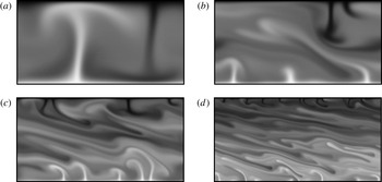
, and non-shearing convection is shown for comparison in figure 2(a). Supplementary movies 1–4 (available at http://dx.doi.org/10.1017/jfm.2014.577) show the time evolution of these four flows. In the non-shearing state, counter-rotating rolls produce rising hot plumes and falling cold ones; these plumes fluctuate but have no mean drift to the left or right. In the shearing states of figure 2(b–d), and especially in supplementary movies 2–4, zonal flows are evidenced by the leftward drift of cold plumes along the top and the rightward drift of hot plumes along the bottom. Top and bottom boundary layers differ instantaneously but not in long-time averages. Although the flows of figure 2(b–d) are all sheared in the same way, their mirror images under the reflection
 $x\mapsto -x$
can arise just as easily; the reflectional symmetry of the governing equations can be broken in either sense. Once the zonal flow has fully developed with one sign or the other, however, we have never seen it reverse at large
 $\mathit{Ra}$
, nor were Krishnamurti & Howard (Reference Krishnamurti and Howard1981) able to induce such reversals in experiments.
Instantaneous temperature fields with
 $\mathit{Pr}=10$
and
 $\mathit{Ra}=2\times 10^{5}$
,
 $2\times 10^{6}$
,
 $2\times 10^{7}$
, and
 $2\times 10^{8}$
(in a–d, respectively). The lowest-
 $\mathit{Ra}$
case (
 $a$
) is non-shearing. The other three cases are examples of sustained shearing convection in which the zonal flow travels leftward along the top boundary and rightward along the bottom one. The hottest fluid (white) is one dimensionless degree warmer than the coldest fluid (black). See also supplementary movies 1–4.

The temperature fields of shearing convection in figure 2(b–d) suggest how zonal flows can persist despite not being directly driven by buoyancy forces. As the fluid in a hot plume rises, it is diverted leftward, first by the sheared mean flow and then by the top boundary, feeding the zonal flow in the upper part of the domain. Likewise, the fluid in a cold plume is diverted rightward as it falls. Put another way, energy created by the action of buoyancy forces cascades upscale, via the velocity nonlinearity, and into the zonal flow. The transfer of energy into the zonal flow is stronger at larger
 $\mathit{Ra}$
, smaller
 $\mathit{Pr}$
, and smaller
 $A$
(Howard & Krishnamurti Reference Howard and Krishnamurti1986; Rucklidge & Matthews Reference Rucklidge and Matthews1996; Goluskin Reference Goluskin2013). These parameter trends are reflected in the linear instability of steady rolls to perturbations of the zonal flow (Thompson Reference Thompson1970; Busse Reference Busse1983; Howard & Krishnamurti Reference Howard and Krishnamurti1986), and they hold also when the zonal flow is dominant, as in the convection studied here.
3.1. Parameter regimes and bistability
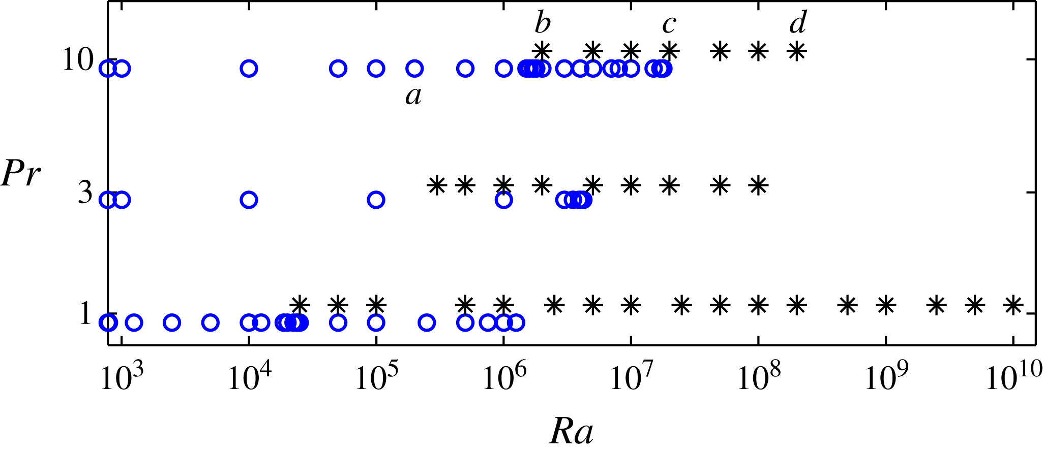
Figure 3 summarizes the parameter values at which we have simulated shearing states (*) and non-shearing states (○) that persist in a domain of aspect ratio 2. The points labelled a–d correspond to the flows shown in figure 2. At each of the three
 $\mathit{Pr}$
simulated, there is a bistable regime in which both shearing and non-shearing states can persist. Non-shearing states in the bistable range of
 $\mathit{Ra}$
can be found by beginning with
 $\mathit{Ra}$
below the range and slowly raising it, while shearing states can be found by beginning with
 $\mathit{Ra}$
above the range and slowly lowering it. It is hard to pinpoint the
 $\mathit{Ra}$
values at which the various solution branches lose stability because transients can be very long, but the data suggest two conclusions: first, that shearing convection is inevitable as
 $\mathit{Ra}\rightarrow \infty$
, and, second, that raising
 $\mathit{Pr}$
also raises the
 $\mathit{Ra}$
at which the transition to shearing convection occurs.
Rayleigh number ranges over which we have found shearing (*) and non-shearing (○) convection to persist with
 $A=2$
and
 $\mathit{Pr}=1$
, 3, or 10. Upper bounds on the non-shearing regimes (
 $\mathit{Ra}=1.2\times 10^{6}$
,
 $3.5\times 10^{6}$
, and
 $1.8\times 10^{7}$
) and the lower bounds on the shearing regimes (
 $\mathit{Ra}=2.5\times 10^{4}$
,
 $3\times 10^{5}$
, and
 $2\times 10^{6}$
) are only approximate. The shearing flows are bursting when
 $\mathit{Pr}=1$
and sustained when
 $\mathit{Pr}=3$
or 10 (see text).

In addition to distinguishing shearing convection from its non-shearing counterpart, we can distinguish between the sustained shearing convection that occurs at larger
 $\mathit{Pr}$
and the bursting shearing convection that occurs at smaller
 $\mathit{Pr}$
. We refer to the sustained flows as such because convective transport is significant at all times, meaning that the instantaneous Nusselt number,
 $N(t)$
, never drops close to unity. We refer to the bursting flows as such because convective transport occurs almost exclusively during discrete bursts, in between which
 $N(t)$
is very close to unity. The distinction between the sustained and bursting types of shearing convection is qualitative, but there is ambiguity only over a narrow transitional range of Prandtl numbers, as described in § 3.4. The present section focuses on sustained shearing convection with
 $\mathit{Pr}=10$
, of which figure 2(b–d) are examples. The shearing convection we have simulated is sustained also when
 $\mathit{Pr}=3$
, whereas it is bursting when
 $\mathit{Pr}=1$
. Bursting shearing convection is the focus of § 4.
The bistable regime shrinks and disappears as the imposed horizontal period,
 $A$
, is decreased. This is consistent with the bifurcation structure of steady states, wherein shearing states arise via supercritical bifurcations when
 $A$
and
 $\mathit{Pr}$
are sufficiently small (Hermiz, Guzdar & Finn Reference Hermiz, Guzdar and Finn1995; Goluskin Reference Goluskin2013; Fitzgerald & Farrell Reference Fitzgerald and Farrell2014). The narrower periods imposed in most prior studies of the full partial differential equations (Rucklidge & Matthews Reference Rucklidge and Matthews1996; Bian et al.
Reference Bian, Benkadda, Garcia, Paulsen and Garbet2003; Garcia & Bian Reference Garcia and Bian2003; Garcia et al.
Reference Garcia, Bian, Paulsen, Benkadda and Rypdal2003) seem to be too narrow for there to be bistability between shearing and non-shearing convection.
3.2. Comparison of integral quantities in shearing and non-shearing convection
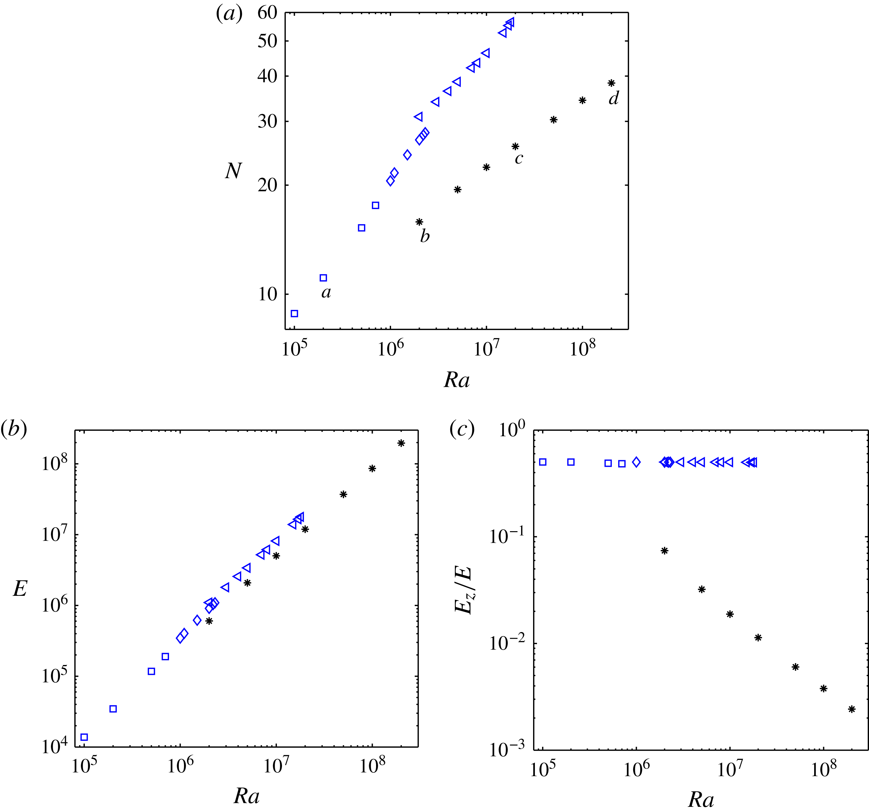
For both shearing and non-shearing solutions, figure 4 shows the Rayleigh-number dependence of time-averaged Nusselt numbers (
 $N$
), total kinetic energies (
 $E$
), and the fractions of these kinetic energies contributed by vertical velocities (
 $E_{z}/E$
). We believe the non-shearing states are variously chaotic, periodic, and quasiperiodic, as indicated in the figure, while the shearing states are all chaotic at this Prandtl number. (Throughout this work, we refer to solutions as quasiperiodic when multiple incommensurable temporal frequencies are present and as chaotic when they appear to have broken all spatial and temporal symmetries of the governing equations. We have not demonstrated that any mathematical definition of chaos is met.) The solutions represented in the temperature fields of figure 2(a–d) are labelled a–d, respectively, in figure 4(a).
(a) Time-averaged Nusselt numbers (
 $N$
), (b) total kinetic energies (
 $E$
), and (c) the fractions of kinetic energies due to vertical velocities (
 $E_{z}/E$
) in sustained shearing convection (*) and non-shearing convection at various Rayleigh numbers for
 $(A,\mathit{Pr})=(2,10)$
. The non-shearing solutions seem to be variously chaotic (▫), periodic (♢), and quasiperiodic (◃), while the shearing solutions all seem to be chaotic. Temperature fields from the cases labelled a–d are shown in figure 2(a–d), respectively.

Some integral quantities, but not all, are significantly affected by zonal flow. Nusselt numbers are smaller and increase more slowly with
 $\mathit{Ra}$
in shearing convection than in non-shearing convection at the same parameters: the Nusselt numbers of the shearing states of figure 4(a) (*) grow approximately like
 $\mathit{Ra}^{0.19}$
, while those of its chaotic non-shearing states (▫) grow like
 $\mathit{Ra}^{0.35}$
. (Heat transport in shearing convection is discussed further in § 5.) Kinetic energies,
 $E$
, grow at similar rates in shearing and non-shearing convection. This is shown for
 $\mathit{Pr}=10$
in figure 4(b) and remains true in our simulations at other Prandtl numbers. However, the fractions of the kinetic energy in the vertical motion,
 $E_{z}/E$
, differ greatly between the two types of flow. In non-shearing convection, horizontal and vertical motions are comparable at all
 $\mathit{Ra}$
, so the fractions remain near
 $\frac{1}{2}$
. In shearing convection,
 $E_{z}/E$
is already smaller than
 $\frac{1}{10}$
when
 $\mathit{Ra}=2\times 10^{6}$
, and it decreases further as
 $\mathit{Ra}$
is raised, even though
 $E_{z}$
itself increases. If this trend continues at very large
 $\mathit{Ra}$
, after the onset of shear turbulence, then
 $E_{z}/E$
will approach zero as
 $\mathit{Ra}\rightarrow \infty$
. In other words, the fraction of kinetic energy in the zonal flow will approach unity.
Energy fluxes shed light on how zonal flow can so greatly change the ways that
 $N$
and
 $E_{z}/E$
depend on
 $\mathit{Ra}$
while hardly changing the dependence of
 $E$
on
 $\mathit{Ra}$
. Averaging
 $\boldsymbol{u}\ \boldsymbol{\cdot }$
(2.2) over space and time yields the time-averaged velocity power integral (Malkus Reference Malkus1954b
; Howard Reference Howard1963),
 $$\begin{eqnarray}\mathit{Ra}(N-1)=\langle |\boldsymbol{{\rm\nabla}}\boldsymbol{u}|^{2}\rangle ^{t}.\end{eqnarray}$$
The left-hand side of expression (3.1) is the mean rate at which the flow gains kinetic energy from buoyancy forces (in suitable units), while the right-hand side is the mean rate at which it loses energy to viscous dissipation. Being equal in the infinite-time limit, either flux can be thought of as the mean energy throughput. Although kinetic energies,
 $E$
, grow with
 $\mathit{Ra}$
at very similar rates in shearing and non-shearing convection, the energy throughput grows more slowly in the shearing case. This is possible because the kinetic energy of shearing convection resides, on average, at larger scales and so dissipates more slowly, meaning the right-hand side of (3.1) is smaller. Correspondingly, less work by buoyancy is needed to maintain the kinetic energy, hence the Nusselt number on the left-hand side of (3.1) is smaller.
3.3. Spatial structure of sustained shearing convection
The vertical structure of sustained shearing convection is markedly different from that of non-shearing convection. In both cases, the thermal boundary layers become thinner as
 $\mathit{Ra}$
is raised, meaning more heat is being conducted upward across them, and the plumes shrink proportionally while becoming more numerous. But, it seems, only in non-shearing convection is the shrinking of the plumes accompanied by their increasing tendency to cluster into composite plumes that can penetrate the whole interior (Parodi et al.
Reference Parodi, von Hardenberg, Passoni, Provenzale and Spiegel2004; von Hardenberg et al.
Reference von Hardenberg, Parodi, Passoni, Provenzale and Spiegel2008). It is evident from the temperature fields of figure 2(b–d) that there is no such clustering in sustained shearing convection. Consequently, as
 $\mathit{Ra}$
is raised, the plumes penetrate less and less far before losing coherence. This is because the mean shear is growing stronger and thus more effective at dispersing plumes horizontally – a phenomenon known as Taylor shear dispersion (Taylor Reference Taylor1953). The dispersion of plumes in shearing convection is more involved than in Taylor’s study because the shear, rather than being imposed a priori, is dynamically driven via the very plumes it helps disperse. When the plumes exceed their time-averaged strength, the zonal flow strengthens and further disperses them; when the plumes fall below this strength, the zonal flow weakens and lets them grow.
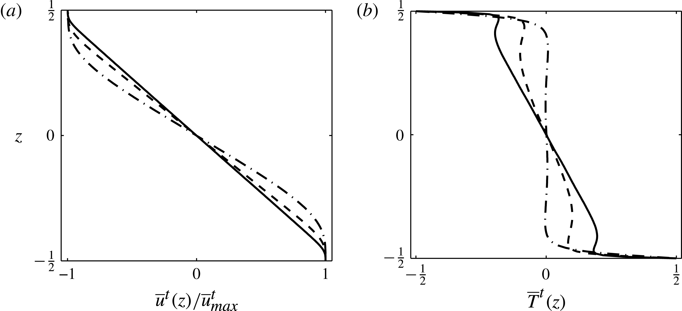
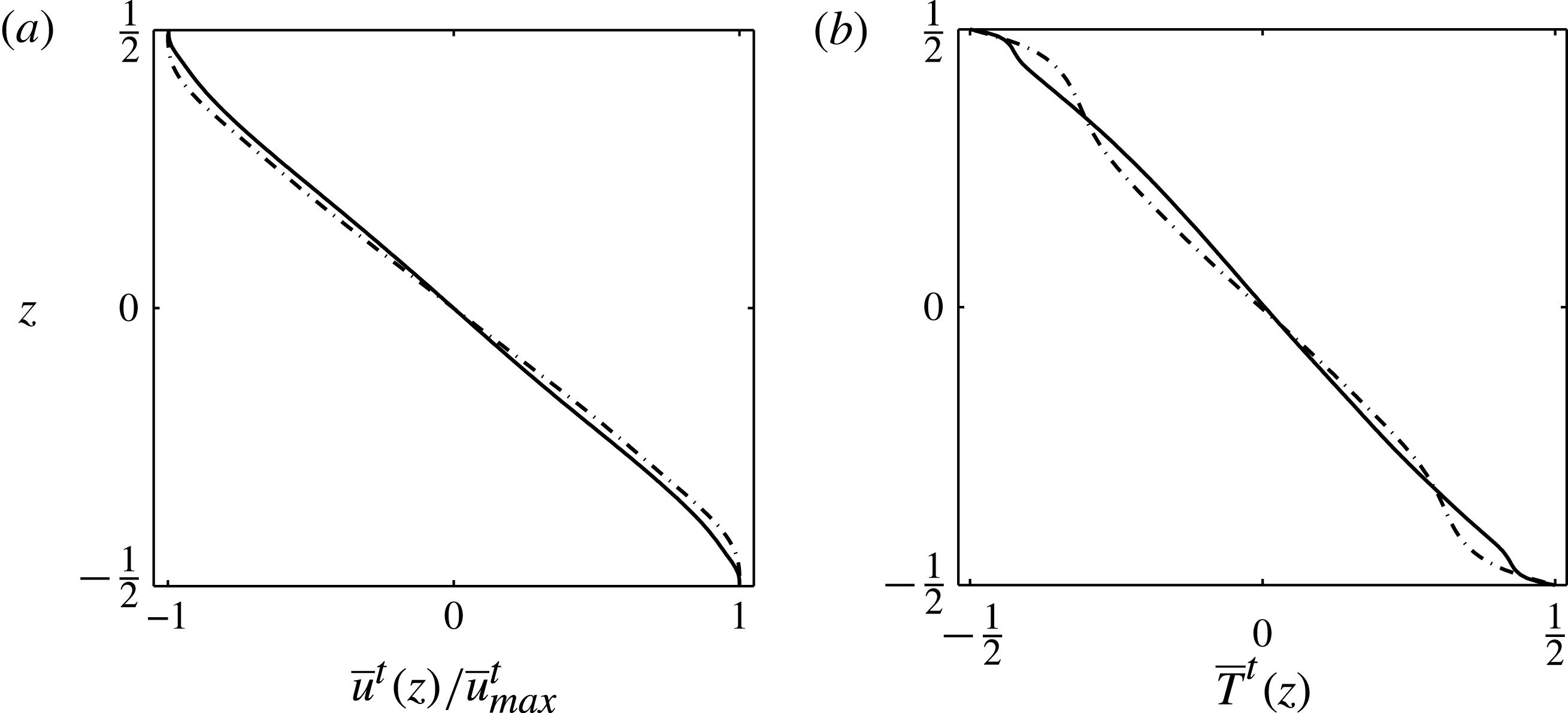
For the three examples of shearing convection visualized in figure 2(b–d), mean vertical profiles of the normalized horizontal velocity,
 $\overline{u}^{t}(z)/\overline{u}_{max}^{t}$
, and the temperature,
 $\overline{T}^{t}(z)$
, are shown in figure 5. All three velocity profiles are roughly linear in the interior, so the shearing of smaller-scale structures by the zonal flow is roughly constant in
 $z$
. This interior region is surrounded by boundary layers in which the shear stresses vanish, as required by the free-slip conditions, and these boundary layers shrink as
 $\mathit{Ra}$
is raised.
Mean vertical profiles of (a) zonal flow and (b) temperature for sustained shearing convection with
 $(A,\mathit{Pr})=(2,10)$
at Rayleigh numbers of
 $2\times 10^{6}$
(– ⋅ – ⋅ –),
 $2\times 10^{7}$
(– – –), and
 $2\times 10^{8}$
(——). Each zonal flow profile is normalized by its maximum value,
 $\overline{u}_{max}^{t}$
. Reversing
 $\overline{u}^{t}(z)$
yields the profiles that arise when symmetry breaks in the opposite way. Figure 9 shows analogous profiles for bursting shearing convection.

Mean temperature profiles in shearing convection are more structured than their non-shearing counterparts. Of the three shearing states represented in figure 5(b), only at the lowest
 $\mathit{Ra}$
, where the zonal flow is weakest, does the
 $\overline{T}^{t}(z)$
profile resemble those of non-shearing convection. That is, there are two thermal boundary layers where heat is transported almost solely by conduction and a nearly isothermal interior where heat is transported almost solely by convection. On the other hand, for the states with
 $\mathit{Ra}=2\times 10^{7}$
and
 $2\times 10^{8}$
, in which the zonal flow is more dominant, we can identify five distinct regions that are delimited by changes in the sign of
 $\text{d}\overline{T}^{t}/\text{d}z$
: two conductive thermal boundary layers, two mixing layers, and the interior.
To interpret the alternating signs of
 $\text{d}\overline{T}^{t}/\text{d}z$
in the profiles of figure 5(b) with
 $\mathit{Ra}=2\times 10^{7}$
and
 $2\times 10^{8}$
, we recall that the time-averaged heat flux is the same across every horizontal plane; only the relative contributions of conduction,
 $-\text{d}\overline{T}^{t}/\text{d}z$
, and convection,
 $\overline{wT}^{t}(z)$
, can change with height, so
 $$\begin{eqnarray}N=-\frac{\text{d}\overline{T}^{t}}{\text{d}z}(z)+\overline{wT}^{t}(z)\end{eqnarray}$$
for all
 $z$
. Just as in non-shearing convection, heat transport in the thermal boundary layers is almost totally conductive. In the mixing layers, defined as the regions where
 $\text{d}\overline{T}^{t}/\text{d}z>0$
, conduction actually carries heat downward but is overmatched by strong upward convection. The vertical extent of these mixing layers roughly corresponds to regions where the plumes are pronounced, as can be seen by comparing figures 2(c,d) and 5(b). In the interior, convection and conduction both contribute to upward heat transport. Some sheared plumes are still discernible there, but they transport less heat than in the mixing layers.
Convection has been studied in which large-scale shear is driven by counter-moving boundaries, rather than by the convection itself. Like the spontaneously arising shear we describe, this imposed shear depresses heat transport at large
 $\mathit{Ra}$
(Lipps Reference Lipps1971; Domaradzki Reference Domaradzki1988; Zaleski Reference Zaleski and Jiménez1991). Temperature profiles reported for systems with counter-moving boundaries resemble their counterparts in non-shearing convection, rather than the more structured profiles we have found with convectively driven shear, but this would be likely to change with stronger imposed shear and larger
 $\mathit{Ra}$
. For Poiseuille–Rayleigh–Bénard convection, where shear is induced by a horizontal pressure gradient, Scagliarini, Gylfason & Toschi (Reference Scagliarini, Gylfason and Toschi2014) report temperature profiles that lack inversions but resemble our own in the interior region.
3.4. Transition between the sustained and bursting regimes of shearing convection
The qualitative distinction between the sustained shearing convection described thus far and the bursting shearing convection described in § 4 is evident in the supplementary movies of evolving temperature fields. It is also evident in time series of various quantities, such as the instantaneous Nusselt number,
 $N(t)$
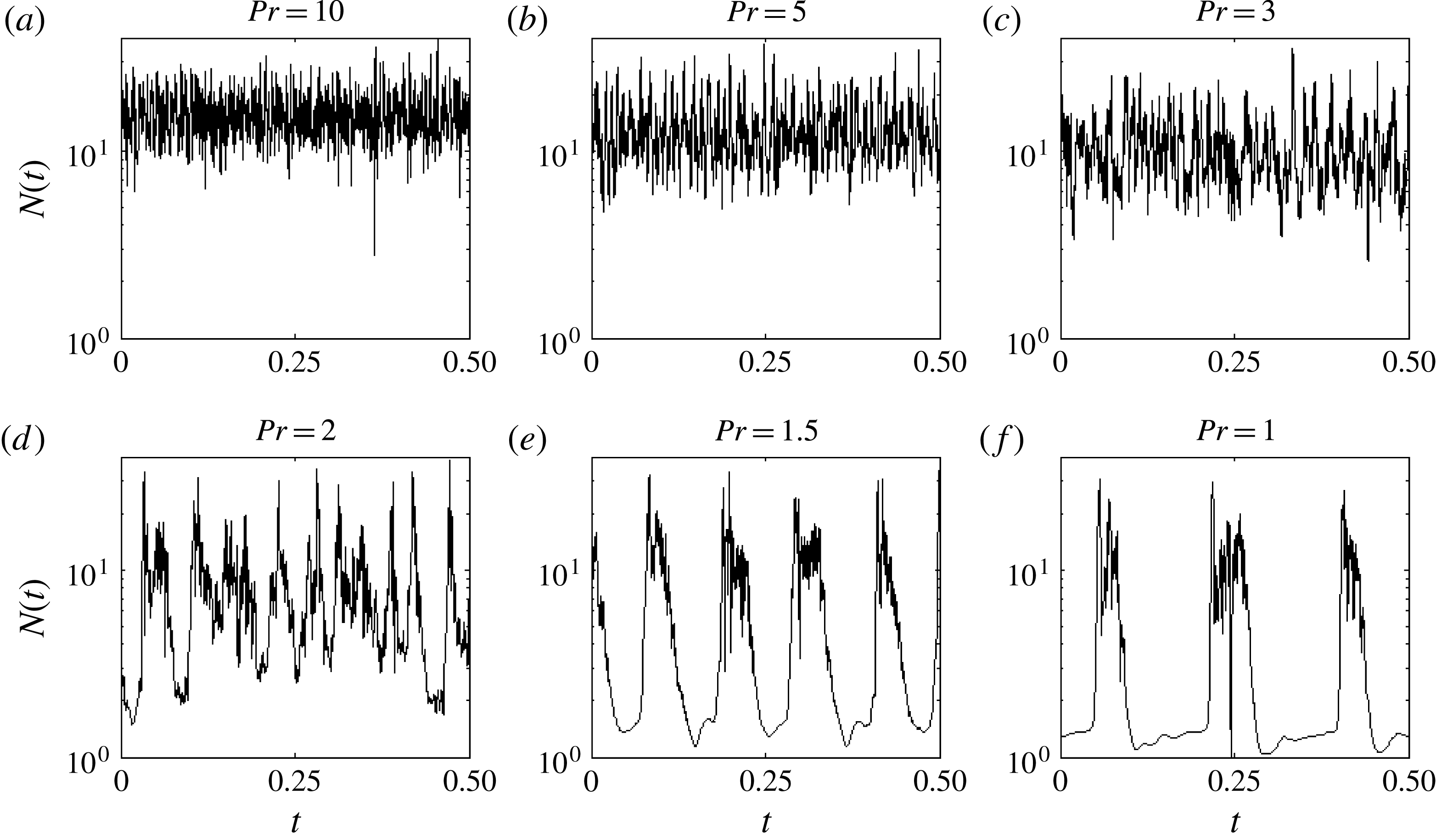
. Figure 6 shows the onset of bursting in
 $N(t)$
as the Prandtl number is lowered from 10 to 1 with
 $\mathit{Ra}=2\times 10^{6}$
. Raising the Prandtl number back through the same values produces similar time series; the transition to bursting seems to be smooth and without hysteresis. At the largest three Prandtl numbers represented in figure 6,
 $N(t)$
remains well above unity at all times, meaning the vertical convection that drives the flow is always significant. This is the sense in which the convection is sustained. Similarly, time series such as
 $E_{x}(t)$
and
 $E_{z}(t)$
in sustained shearing convection deviate only modestly from their time-averaged values (cf. § B.1).
Time series of instantaneous (volume-averaged) Nusselt numbers in shearing convection for six Prandtl numbers between 1 and 10 with
 $(A,Ra)=(2,2\times 10^{6})$
. The transition between the sustained and bursting versions of shearing convection is illustrated.

The fluctuations of
 $N(t)$
in figure 6 intensify as
 $\mathit{Pr}$
is lowered until, when
 $\mathit{Pr}$
is near 1.5, they become so pronounced that
 $N(t)$
begins to ‘bottom out’ near unity. This creates a quiescent phase with little convective transport, punctuated by convective bursts: bursting shearing convection. The transition occurs over a fairly narrow range of
 $\mathit{Pr}$
but not at a well-defined value. Quiescent phases are hinted at (in figure 6) when
 $\mathit{Pr}=2$
, are short when
 $\mathit{Pr}=1.5$
, and are quite pronounced when
 $\mathit{Pr}=1$
. The transition between bursting and sustained shearing convection thus occurs over the approximate range
 $1.5\lesssim \mathit{Pr}\lesssim 2$
when
 $\mathit{Ra}=2\times 10^{6}$
. This range is similar at larger
 $\mathit{Ra}$
, at least up to
 $10^{8}$
.
4. Bursting shearing convection at a moderate Prandtl number
In this section, we examine bursting shearing convection, which we have simulated with
 $(A,\mathit{Pr})=(2,1)$
and Rayleigh numbers in the range
 $2.5\times 10^{4}\leqslant Ra\leqslant 10^{10}$
. Unlike the sustained shearing convection described in § 3, bursting flows at a Prandtl number of unity have been simulated previously (Bian et al.
Reference Bian, Benkadda, Garcia, Paulsen and Garbet2003; Garcia & Bian Reference Garcia and Bian2003; Garcia et al.
Reference Garcia, Bian, Paulsen, Benkadda and Rypdal2003; van der Poel et al.
Reference van der Poel, Ostilla-Mónico, Verzicco and Lohse2014). Moreover, exactly periodic bursts have been seen in reduced models that account for zonal flow (Leboeuf, Charlton & Carreras Reference Leboeuf, Charlton and Carreras1993; Malkov, Diamond & Rosenbluth Reference Malkov, Diamond and Rosenbluth2001; Bian & Garcia Reference Bian and Garcia2003), and less pronounced bursts can occur even when the large-scale shear is driven directly by boundary motion (Zaleski Reference Zaleski and Jiménez1991). We add to past findings here by simulating a wider range of Rayleigh numbers in a larger domain.
4.1. The physics of a burst
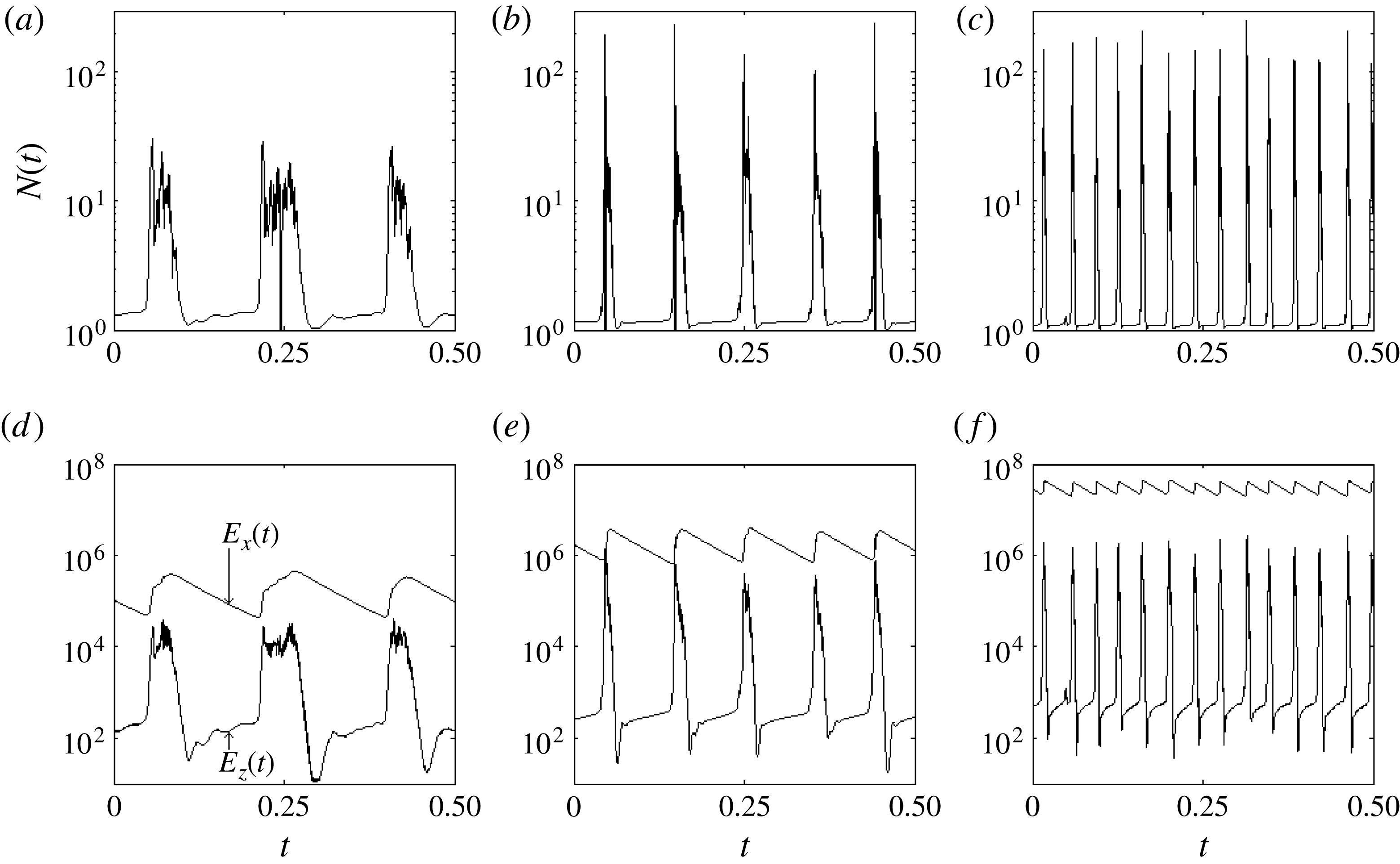
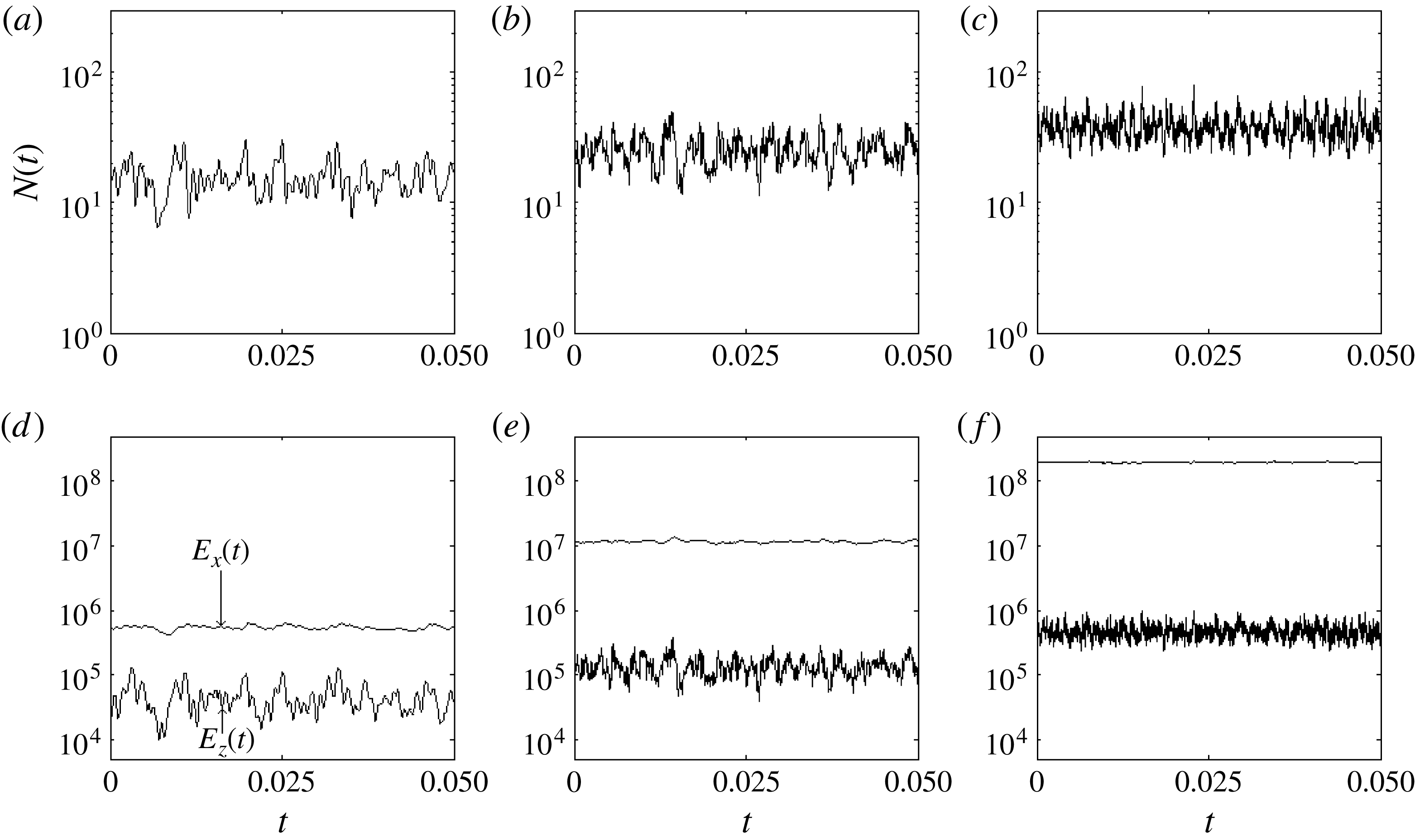
Figure 7 shows time series of
 $N(t)$
,
 $E_{x}(t)$
, and
 $E_{z}(t)$
for bursting shearing convection with
 $\mathit{Ra}=2\times 10^{6}$
,
 $2\times 10^{7}$
, and
 $2\times 10^{8}$
. These are the same three Rayleigh numbers as in the examples of sustained shearing convection in § 3; only the Prandtl number has changed (from 10 to 1), as described in § 3.4. In each time series of figure 7, the quiescent phase is punctuated by global bursts that are much stronger than the flow’s local fluctuations and have a much lower mean frequency. All three quantities in figure 7 rise quickly during a burst, after which
 $N(t)$
and
 $E_{z}(t)$
return quickly to their quiescent values, while
 $E_{x}(t)$
relaxes until the next burst. For the case with
 $\mathit{Ra}=2\times 10^{8}$
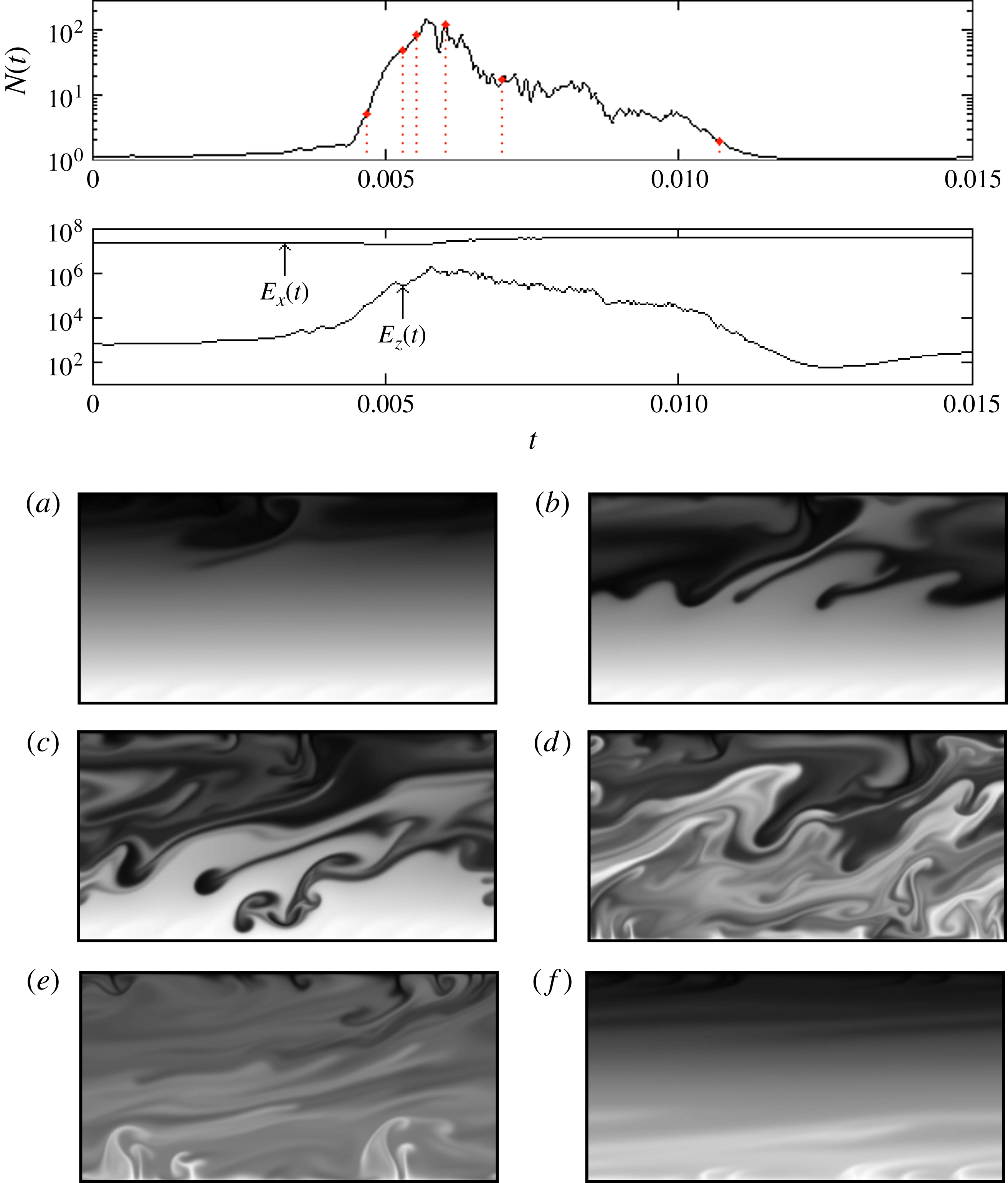
, the life cycle of a single burst is illustrated in figure 8, where
 $N(t)$
is shown alongside six representative temperature fields.
Time series of (a–c) the Nusselt numbers and (d–f) the kinetic energies of the horizontal velocities (
 $E_{x}$
, upper curves) and vertical velocities (
 $E_{z}$
, lower curves) in bursting shearing convection with
 $(A,\mathit{Pr})=(2,1)$
. The three Rayleigh numbers represented are
 $2\times 10^{6}$
(a,d),
 $2\times 10^{7}$
(b,e), and
 $2\times 10^{8}$
(c, f). The integral quantities are as defined in expressions (2.9a,b
) and (2.10) but with time averages not taken.

Time series of
 $N(t)$
,
 $E_{x}(t)$
, and
 $E_{z}(t)$
during a single burst, along with six instantaneous temperature fields, with
 $(\mathit{Pr},Ra)=(1,2\times 10^{8})$
. The time origin is arbitrary, and the full quiescent phases are not shown. The instants represented in fields (a)–(f) are marked from left to right, respectively, by vertical dashed lines on the time series of
 $N(t)$
. The hottest fluid (white) is one dimensionless degree warmer than the coldest fluid (black). See also supplementary movie 5.

The physics behind the bursts of figure 7 has been discussed before (Leboeuf et al.
Reference Leboeuf, Charlton and Carreras1993; Garcia et al.
Reference Garcia, Bian, Naulin, Nielsen and Rasmussen2006) and can be interpreted with the help of the three integral quantities shown. During the quiescent phase, there is little convective motion, so
 $N(t)\approx 1$
and
 $E_{z}(t)\ll E_{x}(t)$
. The small Nusselt number means that buoyancy is doing very little work on the fluid, so
 $E_{x}(t)$
relaxes towards zero. As convective structures are dispersed more and more, the vertical temperature profile comes very close to being linear, and the gravest zonal mode,
 $u\propto \sin {\rm\pi}z$
, dominates the flow because it decays the most slowly. That is,
 $$\begin{eqnarray}\displaystyle & T\approx -z, & \displaystyle\end{eqnarray}$$
 $$\begin{eqnarray}\displaystyle & (u,w)\approx (c\text{e}^{-{\rm\pi}^{2}\mathit{Pr}\,t}\sin {\rm\pi}z,0), & \displaystyle\end{eqnarray}$$
 $c$
is a constant that depends on the time origin and the parameters. At the large Rayleigh numbers under study, this conductive temperature profile would be highly unstable if the fluid were at rest. When the zonal flow has significant momentum, however, it suppresses the convective instability, so convection does not return until the zonal flow has decayed sufficiently. This same mechanism raises the critical Rayleigh number of linear instability when steady shear is imposed on the two-dimensional RB model (Deardorff Reference Deardorff1965; Gallagher & Mercer Reference Gallagher and Mercer1965; Ingersoll Reference Ingersoll1966).
Bursts begin when the zonal flow becomes too weak to suppress the usual mechanism of convective instability, at which time
 $N(t)$
and
 $E_{z}(t)$
quickly grow, and the fluid overturns, as shown in figure 8(b–d) and supplementary movie 5. Thermal plumes return, and the fluid is once again energized as buoyancy drives circulation. However, the newfound kinetic energy is quickly transferred into the zonal flow, which then shuts off the
 $N(t)$
and
 $E_{z}(t)$
bursts as a new quiescent phase begins.
To see the bursting from the perspective of dynamical systems, we can note that the relaxation defined by expressions (4.1) and (4.2) solves the governing equations exactly and lies in the stable manifold of the static state. During the quiescent phase, the flow is close to this exact solution. Each burst carries the system away from the relaxing solution and then back towards it, leaving the flow with more energy (that is, farther from the static equilibrium). Similar behaviour has been called on–off intermittency (Platt, Spiegel & Tresser Reference Platt, Spiegel and Tresser1993), one of several types of fluid dynamical bursting surveyed by Knobloch & Moehlis (Reference Knobloch, Moehlis, Golubitsky, Luss and Strogatz1999).
Yet another way to view bursting shearing convection is by analogy with the oscillations of predator and prey populations in the Lotka–Volterra equations, a pair of first-order ordinary differential equations (Lotka Reference Lotka1925). Several authors have spoken in these terms, and a few have even derived predator–prey-type equations from the Boussinesq equations under various closure assumptions (Leboeuf et al. Reference Leboeuf, Charlton and Carreras1993; Malkov et al. Reference Malkov, Diamond and Rosenbluth2001; Bian & Garcia Reference Bian and Garcia2003).
4.2. Dependence of bursts on the Rayleigh number
The bursts shown in figure 7 change in several ways as
 $\mathit{Ra}$
is raised. They become more frequent, relative to the timescale of thermal diffusion by which we have non-dimensionalized, and more extreme. In our simulations of sustained shearing convection, on the other hand,
 $N(t)$
and
 $E_{z}(t)$
fluctuate less strongly as
 $\mathit{Ra}$
is raised, and the fluctuations in
 $E_{x}(t)$
are scarcely perceptible (cf. § B.1).
The dependence of the time-averaged Nusselt number,
 $N$
, on
 $\mathit{Ra}$
is not obvious from the time series of
 $N(t)$
in figure 7. Raising
 $\mathit{Ra}$
makes the bursts of
 $N(t)$
stronger and more frequent but also shorter-lived, and these trends are in opposition. As reported in § 5, the trends are in close competition, so
 $N$
changes only very gradually over several decades of
 $\mathit{Ra}$
.
4.3. Vertical and temporal structure
Thermal plumes are localized in time in bursting shearing convection, whereas they are localized in space in the sustained shearing convection of § 3. In the sustained case, the supplementary movies accompanying figure 2 illustrate that plumes exist at all times but have limited vertical extent, and we have identified this extent with the regions of positive temperature gradient, here called mixing layers, in the
 $\overline{T}^{t}(z)$
profiles of figure 5(b). In the bursting case, there are no mixing layers; figure 8 and the accompanying supplementary movie 5 show that plumes penetrate the entire layer during bursts and are almost totally dispersed in between. Time-averaging over the bursts yields
 $\overline{T}^{t}(z)$
profiles that are fairly close to linear, as shown in figure 9(b), with the deviation from linearity near the boundaries being created almost entirely by the bursts. On the other hand, the normalized zonal flow profiles, shown for the bursting case in figure 9(a), are similar to their sustained counterparts in figure 5(a).
Mean vertical profiles of (a) zonal flow and (b) temperature for bursting shearing convection with
 $(A,\mathit{Pr})=(2,1)$
at Rayleigh numbers of
 $2\times 10^{6}$
(– ⋅ – ⋅ –) and
 $2\times 10^{8}$
(——). Each zonal flow profile is normalized by its maximum value,
 $\overline{u}_{max}^{t}$
. Reversing
 $\overline{u}^{t}(z)$
yields the profiles that arise when symmetry breaks in the opposite way. Figure 5 shows analogous profiles for sustained shearing convection.

5. Nusselt numbers
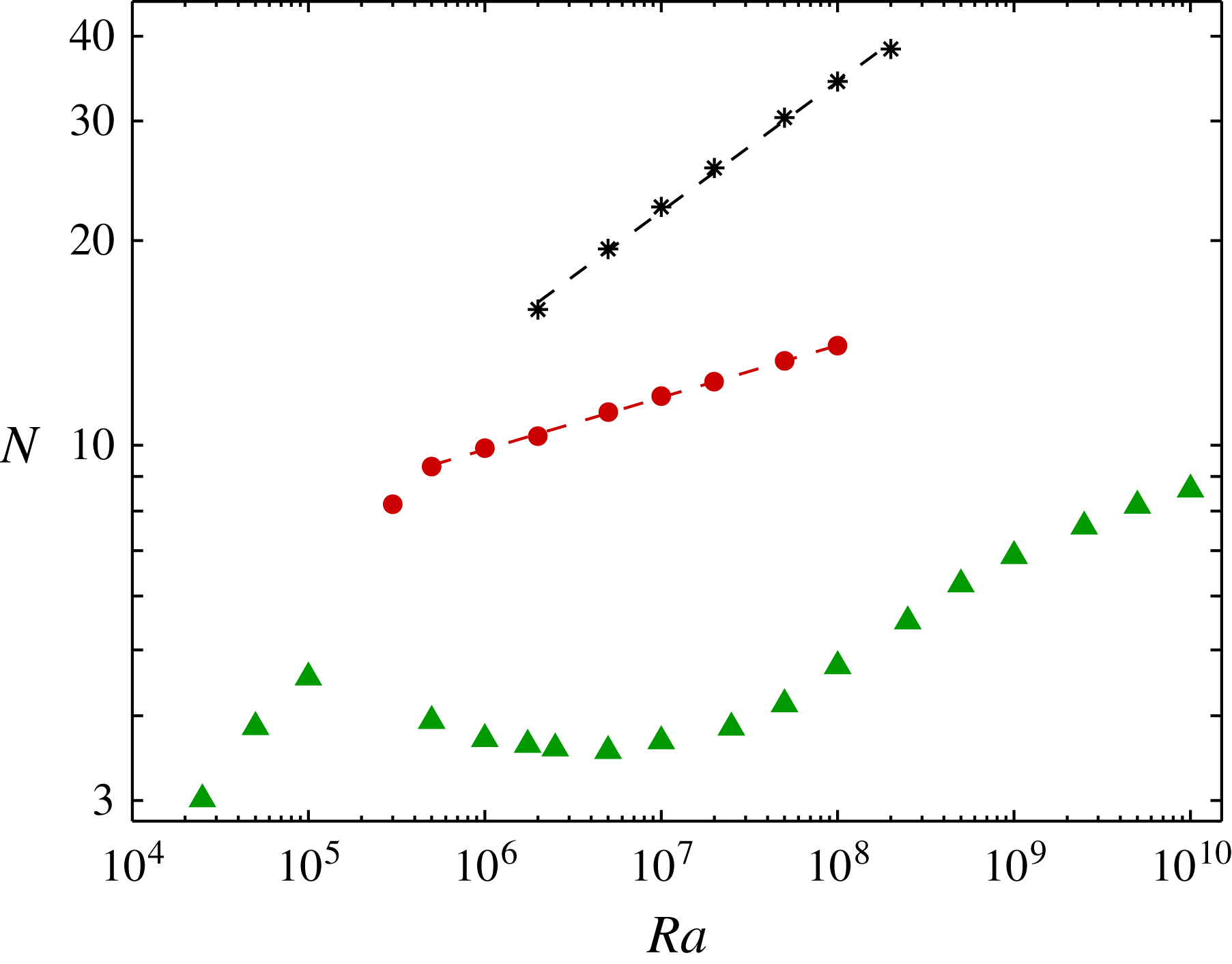
Our findings on the mean Nusselt numbers of shearing convection are summarized in figure 10, where the dependence of
 $N$
on
 $\mathit{Ra}$
is shown for Prandtl numbers of 1 (▴), 3 (●), and 10 (*). The shearing convection is bursting when
 $\mathit{Pr}=1$
and sustained when
 $\mathit{Pr}=3$
or 10, as illustrated in figure 6 for the particular Rayleigh number of
 $2\times 10^{6}$
. At each
 $\mathit{Pr}$
, we found no shearing states at lower
 $\mathit{Ra}$
than shown in figure 10.
Mean Nusselt numbers,
 $N$
, of shearing convection at three Prandtl numbers and various Rayleigh numbers in a domain with
 $A=2$
. The shearing convection is bursting with
 $\mathit{Pr}=1$
(▴) and sustained with
 $\mathit{Pr}=3$
(●) and
 $\mathit{Pr}=10$
(*). In the sustained cases, dashed lines show power-law fits of
 $N\sim 3.4\,Ra^{0.077}$
for
 $\mathit{Pr}=3$
and
 $N\sim 1.0\,Ra^{0.19}$
for
 $\mathit{Pr}=10$
. These
 $N$
values are compared to those of non-shearing states for
 $\mathit{Pr}=10$
and
 $\mathit{Pr}=1$
in figures 4 and 12, respectively.

The sharp change in the
 $\mathit{Pr}=1$
data of figure 10 seems to correspond to a transition from quasiperiodic states (in the three flows with lowest
 $\mathit{Ra}$
) to chaotic bursting. We have found no quasiperiodic states with
 $\mathit{Pr}=10$
, where shearing convection sets in at larger
 $\mathit{Ra}$
. With
 $\mathit{Pr}$
smaller than unity, on the other hand, shearing convection sets in at smaller
 $\mathit{Ra}$
and can be quasiperiodic, periodic, or even steady (Rucklidge & Matthews Reference Rucklidge and Matthews1996; Goluskin Reference Goluskin2013). Such highly symmetric shearing states exist also at the parameters studied here but do not arise in simulations because they are unstable.
When
 $\mathit{Pr}$
is smaller, the minimum Rayleigh number needed for shearing convection is also smaller. This is borne out not only by the
 $\mathit{Ra}$
at which shearing convection persists in direct numerical simulations (cf. figure 10) but also by the
 $\mathit{Ra}$
at which steady shearing states come into existence (Rucklidge & Matthews Reference Rucklidge and Matthews1996). These steady states exist at the parameters studied here but do not arise in simulations because they are unstable. Steady shearing states that are stable have been found in our geometry only when
 $\mathit{Pr}\lesssim 0.3$
(Goluskin Reference Goluskin2013). At somewhat larger
 $\mathit{Pr}$
, shearing states that are periodic or quasiperiodic in time can be stable. Of the states represented in figure 10, it appears that the first with
 $\mathit{Pr}=3$
and the first three with
 $\mathit{Pr}=1$
are quasiperiodic, while the rest are chaotic. A more thorough study of these transitional states could be better carried out using the tools of numerical bifurcation analysis.
For all three Prandtl numbers represented in figure 10, the dependence of
 $N$
on
 $\mathit{Ra}$
in shearing convection is unlike any reported for ordinary (non-shearing) RB convection. In the bursting shearing convection with
 $\mathit{Pr}=1$
,
 $N$
varies non-monotonically with
 $\mathit{Ra}$
, decreasing in the range
 $10^{5}\lesssim Ra\lesssim 2.5\times 10^{6}$
before continuing to increase. This range of decrease is quite unusual, and we are not aware of a precedent. In the sustained shearing convection, the Nusselt number grows roughly as a power of the Rayleigh number: our measured
 $N$
are best-fit by power laws proportional to
 $\mathit{Ra}^{0.077}$
when
 $\mathit{Pr}=3$
and to
 $\mathit{Ra}^{0.19}$
when
 $\mathit{Pr}=10$
. In the study of ordinary RB convection, many such power laws have been fitted to measured
 $N$
and
 $\mathit{Ra}$
, but the powers are always larger, ranging from
 $\frac{1}{5}$
to
 $\frac{1}{2}$
(Grossmann & Lohse Reference Grossmann and Lohse2000; Ahlers et al.
Reference Ahlers, Grossmann and Lohse2009).
The only prior result on the scaling of
 $N(Ra,\mathit{Pr})$
in shearing convection, as far as we know, appears in the plasma-motivated work of Garcia et al. (Reference Garcia, Bian, Paulsen, Benkadda and Rypdal2003), who simulated bursting shearing convection in a square domain with
 $\mathit{Pr}=1$
. Defining a suitable
 $N$
and
 $\mathit{Ra}$
for their thermal boundary conditions, we find that their
 $N$
grew monotonically (though slowly) with
 $\mathit{Ra}$
, contrary to our findings at the same Prandtl number. As discussed in § B.2, this difference might be caused by their narrower domain.
We have not found scaling arguments for
 $N(Ra,\mathit{Pr})$
in shearing convection that are consistent with the data of figure 10. It may be easier to first study
 $N(Ra,\mathit{Pr})$
in non-shearing RB convection between free-slip boundaries. Such convection has received much less attention than its no-slip counterpart, but the importance of velocity boundary conditions is hinted at by analytical upper bounds on
 $N$
, whose scalings with
 $\mathit{Ra}$
can depend on the boundary conditions (Otero et al.
Reference Otero, Wittenberg, Worthing and Doering2002; Plasting & Ierley Reference Plasting and Ierley2005; Ierley, Kerswell & Plasting Reference Ierley, Kerswell and Plasting2006; Whitehead & Doering Reference Whitehead and Doering2011, Reference Whitehead and Doering2012). In particular,
 $N$
cannot grow faster than
 $\mathit{Ra}^{5/12}$
when the boundaries are free-slip and the flow is two-dimensional (Whitehead & Doering Reference Whitehead and Doering2011), so the flow cannot achieve the ultimate scaling of
 $\mathit{Ra}^{1/2}$
that is expected when the boundaries are no-slip (Kraichnan Reference Kraichnan1962; Spiegel Reference Spiegel1971b
). A viable alternative is the ultimate scaling of
 $\mathit{Ra}^{1/3}$
suggested by the argument, due to Priestly (see Spiegel Reference Spiegel1971a
), that
 $N$
should not depend on the layer thickness in the infinite-
 $\mathit{Ra}$
limit. At large but non-ultimate
 $\mathit{Ra}$
, however, we are not aware of scaling arguments for RB convection between free-slip boundaries, be it shearing or non-shearing.
6. Conclusions
Large-scale shear in RB convection is of interest not only because the RB model is an exemplar of complexity, but also because the interplay between convection and mean shear captures some aspects of more complicated astrophysical and plasma-physical applications. We have studied the phenomenon by simulating a configuration in which it is especially pronounced; the free-slip boundaries and horizontal periodicity let mean horizontal flow travel unimpeded, and the two-dimensionality prevents disruption by motions transverse to the mean flow. When large-scale shear is present, we have referred to the total state as shearing convection and to its mean horizontal component as the zonal flow.
Although large-scale shear has been seen in laboratory convection (for instance, by Malkus Reference Malkus1954a ; Krishnamurti & Howard Reference Krishnamurti and Howard1981), the shear we have examined is different. Simulations with horizontal periodicity, which is impossible in Cartesian laboratory experiments, allow for mean flows with horizontal wavenumbers of zero – the so-called zonal flows. These flows can account for a large fraction of the total kinetic energy and can significantly depress the vertical heat transport. Their name is adopted from the zonal flows that are seen in planetary atmospheres and tokamaks, and with which they share several features.
A direct comparison between shearing and non-shearing convection is possible in parameter regimes where states of both types are bistable, and such regimes exist for all Prandtl numbers between 1 and 10 that we have simulated in our chosen geometry. Shearing states are distinguished by the fact that plumes on opposing boundaries drift in opposite directions, as well as by the values of key integral quantities. Remarkably, the fraction of the total kinetic energy that the zonal flow accounts for tends towards unity as
 $\mathit{Ra}\rightarrow \infty$
. The resulting large-scale shear helps disperse thermal plumes, thereby reducing heat transport. Nusselt numbers in shearing convection, compared to those of non-shearing convection, are smaller and grow more slowly with
 $\mathit{Ra}$
, if they grow at all. Large-scale shear has been credited with depressing Nusselt numbers in a number of RB experiments (such as those of Castaing et al.
Reference Castaing, Gunaratne, Heslot, Kadanoff, Libchaber, Thomae, Wu, Zaleski and Zanetti1989; Werne Reference Werne1993), but the effect is more more pronounced here. It more resembles the dramatic reduction of heat transport that is possible when shear is imposed at the boundaries, rather than arising as a secondary flow (Lipps Reference Lipps1971; Domaradzki Reference Domaradzki1988; Zaleski Reference Zaleski and Jiménez1991).
Shearing convection at large Rayleigh numbers exhibits one of two forms of time dependence. In what we call sustained shearing convection, which occurs in our simulations when the Prandtl number is larger than about 2, vertical convective transport is significant at all times. In bursting shearing convection, which occurs at smaller Prandtl numbers, convective transport is confined to discrete bursts that resemble on–off intermittency (Platt et al. Reference Platt, Spiegel and Tresser1993). The bursting form of shearing convection has been described before, as surveyed by Garcia et al. (Reference Garcia, Bian, Naulin, Nielsen and Rasmussen2006), whereas it seems that the sustained form has not. The zonal flow may be thought of as a parasite, draining energy from its convective host. In the sustained case, buoyancy forces are able to energize the host flow as quickly as the zonal flow parasitizes it. In the bursting case, the parasite drains energy too quickly, creating bursts as the host flow plummets and rebounds.
Several astrophysical questions may benefit from an improved understanding of shearing convection. For instance, helioseismic studies have revealed large-scale horizontal flows at the top and the bottom of the solar convection zone, and convection may play a role in driving them. The convective cores of massive stars rotate rapidly and so might also be poised to produce large-scale shear. If so, the shear is likely to influence the lifetimes and internal structures of the stars since it has been found to augment reaction rates (Spiegel & Zaleski Reference Spiegel and Zaleski1984), much as it augments diffusion.
In tokamak plasmas, zonal flow is central to the effort to confine fusion magnetically (Wagner Reference Wagner2007). Since tokamaks cannot yet be simulated under operating conditions, the construction of increasingly large experiments is justified, in part, by extrapolating past results. It is crucial that enlarging the tokamak does not significantly enhance the interchange motions that harm confinement, at least in the ‘high-confinement mode’ where zonal flow is present. The analogous behaviour in the RB system would be the Nusselt number of shearing convection holding steady as
 $\mathit{Ra}$
is raised. However, this is not what we observe: zonal flow slows, but often does not stop, the growth of the Nusselt number with
 $\mathit{Ra}$
. This is especially true of the sustained form of shearing convection, which more resembles the high-confinement mode. (The bursting form of shearing convection has instead been likened to edge-localized modes in tokamaks (Finn Reference Finn1993; Leboeuf et al.
Reference Leboeuf, Charlton and Carreras1993; Horton, Hu & Laval Reference Horton, Hu and Laval1996).) The analogy between tokamaks and RB convection is only qualitative, and we cannot say how well it holds up. If taken at face value, our findings suggest that interchange motions would become increasingly harmful in ever-larger tokamaks, even in the high-confinement mode.
Open questions surround even basic features of large-scale shear in RB convection. Mapping out the parameter regimes in which shearing convection can be stable is not easy; the states in question are apparently chaotic when the domain is wide or the Prandtl number large, so transitions are hard to locate precisely, though our simulations give some estimates. Domains wider than ours have not been explored, and it is unclear how readily large-scale shear will persist in very wide domains. Once shearing convection is found in a region of parameter space, we can gain some insight into its character from integral quantities like the heat flux and the energy of the zonal flow. Beyond the data we have reported, little is known about the parameter-dependence of these quantities. An especially intriguing question is the fate of the Nusselt number in the infinite-
 $\mathit{Ra}$
limit. The ultimate scaling of
 $N\propto Ra^{1/2}$
conjectured for no-slip boundaries is ruled out for free-slip boundaries in two dimensions (Whitehead & Doering Reference Whitehead and Doering2011), and even the unbounded growth of
 $N$
is not assured in shearing convection. Perhaps the real moral of our tale is that thermal convection continues to yield new aspects after centuries of study. It will no doubt remain a model of complexity for quite some time.
Acknowledgements
We are grateful for the interest and conversation of C. Doering, E. van der Poel, J. Whitehead, J. Aurnou, K. Julien, and E. Knobloch, and for the suggestions of the anonymous referees. D. Zhu, in collaboration with G.R.F., performed many simulations with heat fluxes, rather than temperatures, fixed at the boundaries and found similar behaviour to what we have reported. The 2010 GFD summer program at the Woods Hole Oceanographic Institute was instrumental in our undertaking of this work. E.A.S. thanks A. Provenzale for some apposite remarks. D.G. is grateful for the general support of D. Keyes and for the guidance of P. Fischer and A. Obabko in running nek5000. D.G. was supported during part of this work by NSF project EMSW21 – RTG: Numerical Mathematics for Scientific Computing (award no. DMS-0602235). Some computing resources were provided by the New York Center for Computational Sciences at Stony Brook University/Brookhaven National Laboratory, which is supported by the DOE (contract no. DE-AC02-98CH10886) and by the State of New York. G.R.F. was supported by NSF collaborative proposal Models of the Deep Circulation of Gas Giants: Solar Heating, Convection, and Zonal Flows (award no. AST-0708106).
Supplementary movies
Supplementary movies are available at http://dx.doi.org/10.1017/jfm.2014.577.
Appendix A. Computational details
Simulations were carried out using both the nek5000 spectral element code (Fisher et al.
Reference Fisher, Lottes and Kerkemeier2014) and a fully spectral collocation code modified from that used by Johnston & Doering (Reference Johnston and Doering2009). The two codes were verified against one another by simulating bursting shearing convection with
 $\mathit{Pr}=1$
and
 $\mathit{Ra}\leqslant 10^{7}$
. At each
 $\mathit{Ra}$
, time-averaged Nusselt numbers agreed to at least two significant figures and usually to three. Bursting flows with
 $\mathit{Ra}>10^{7}$
, which are the most numerically challenging flows studied here, were simulated using only the fully spectral code. Higher-
 $\mathit{Pr}$
flows, which do not burst and are less numerically challenging, were simulated primarily using nek5000 because the code scales well to large numbers of processors, though some cases were verified using the spectral code also.
The nek5000 code was configured for second-order variable time stepping with a target Courant number of
 $\frac{1}{2}$
. Without bursting, time averages were deemed converged after a time span,
 ${\it\tau}$
, when cumulative averages of the Nusselt number and kinetic energy,
 $N$
and
 $E$
, agreed with their values after
 ${\it\tau}/2$
to within 0.2 %. Spatial meshes, composed of square and uniform elements, were deemed converged when increasing the polynomial order of each element by 2 changed
 $N$
and
 $E$
by less than 1 %. Most simulations were performed in a domain of aspect ratio
 $A=2$
with
 $64\times 32$
elements. Elements of polynomial order 8 were needed when
 $\mathit{Ra}\geqslant 10^{8}$
, while elements of order 6 or 4 sufficed at smaller
 $\mathit{Ra}$
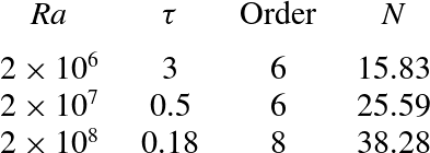
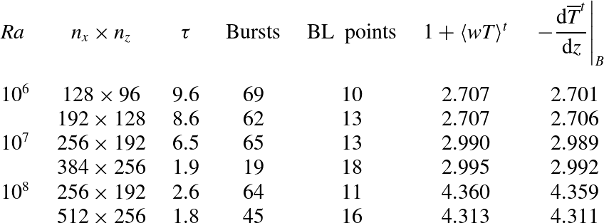
. Table 1 gives representative parameters and Nusselt numbers for simulations of sustained shearing convection with
 $(A,\mathit{Pr})=(2,10)$
.
The meshes needed to resolve sustained shearing convection are much coarser than demanded by non-shearing convection at similar
 $\mathit{Ra}$
, and guidelines based on ordinary RB convection (Shishkina et al.
Reference Shishkina, Stevens, Grossmann and Lohse2010) overestimate the resolution needed for our
 $N$
and
 $E$
to converge. This is reasonable since the shear leads to thicker thermal boundary layers, and it disperses fine structures. To further check mesh convergence in our nek5000 simulations, the three highest-
 $\mathit{Ra}$
simulations were repeated using the fully spectral code, and
 $N$
was computed using four different expressions that should agree in the infinite-time limit. The results for
 $\mathit{Ra}=2\times 10^{8}$
are shown in table 2. Among both codes, both spectral meshes, and all four methods of calculating
 $N$
, the greatest per cent error was less than 1 %.
The spectral collocation scheme we used to simulate the bursting shearing convection of § 4 uses a Fourier basis in
 $x$
and a Chebyshev basis in
 $z$
. The method is as described by Johnston & Doering (Reference Johnston and Doering2009), except that we impose free-slip conditions here. Since the scheme integrates the vorticity–stream function (
 ${\it\omega}$
–
 ${\it\psi}$
) formulation of (2.1)–(2.3), impenetrable free-slip conditions are enforced easily by
 $$\begin{eqnarray}{\it\omega}={\it\psi}=0\quad \text{at }z=\pm {\textstyle \frac{1}{2}}.\end{eqnarray}$$
A tensor product of dimensions
 $n_{x}\times n_{z}$
was used for the spatial mesh. When
 $n_{z}\geqslant 128$
, the ordinary Chebyshev spacing in
 $z$
was modified by a coordinate mapping similar to that of Kosloff & Tal-Ezer (Reference Kosloff and Tal-Ezer1993). When
 $n_{x}\geqslant 256$
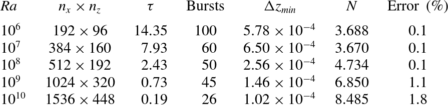
, an eighth-order exponential filter was used to control aliasing errors in the convection term. Table 3 gives representative parameters and Nusselt numbers for simulations of bursting shearing convection with
 $(A,\mathit{Pr})=(2,1)$
. Time averages were deemed converged after a time span,
 ${\it\tau}$
, when
 $N$
and
 $E$
agreed with their values after
 ${\it\tau}/2$
to within 2 %. Spatial resolution was tested in a square domain (
 $A=1$
) for
 $\mathit{Ra}\leqslant 10^{8}$
, and meshes were deemed converged when increasing the resolution by
 $\frac{1}{3}$
changed
 $N$
by less than 1.5 %. Table 4 gives the results of these resolution tests.
Representative parameters for simulations, using nek5000, of sustained shearing convection with
 $(A,\mathit{Pr})=(2,10)$
. Quantities shown for each
 $\mathit{Ra}$
are the dimensionless runtime after transients (
 ${\it\tau}$
), element order, and time-averaged
 $N$
. All three simulations used a uniform mesh of
 $64\times 32$
square elements. These three flows are used as examples throughout § 3 and in figure 11.

Verification of the Nusselt number in sustained shearing convection with
 $(A,\mathit{Pr},Ra)=(2,10,2\times 10^{8})$
. Tabulated quantities include the mesh size (
 $n_{x}\times n_{z}$
), dimensionless runtime after transients (
 ${\it\tau}$
), the estimated number of points in the thermal boundary layer, and four expressions for
 $N$
that should be equal in the infinite-time limit.

Representative parameters for simulations, using the spectral collocation code, of bursting shearing convection with
 $(A,\mathit{Pr})=(2,1)$
. Quantities shown for each
 $\mathit{Ra}$
are the mesh size (
 $n_{x}\times n_{z}$
), dimensionless runtime after transients (
 ${\it\tau}$
), number of bursts, minimum
 $z$
-spacing of the mapped mesh (
 ${\rm\Delta}z_{min}$
), Nusselt number (
 $N$
), and the relative error between
 $N$
after runtime
 ${\it\tau}/2$
and after runtime
 ${\it\tau}$
. Values of
 $N$
computed using the temperature gradient at a boundary, instead of using
 $1+\langle wT\rangle ^{t}$
, differ by less than 1 %.

Appendix B. Supplementary results
B.1. Time series for sustained shearing convection with
 $\mathit{Pr}=10$

Figure 11 shows time series of
 $N(t)$
,
 $E_{x}(t)$
, and
 $E_{z}(t)$
for the three examples of sustained shearing convection whose temperature fields and time-averaged properties are explored in § 3. These series may be contrasted with the bursting time series shown in figure 7. Only fast local fluctuations are present in figure 11, as opposed to bursts, and all three quantities fluctuate less strongly as
 $\mathit{Ra}$
is raised.
Time series of (a–c) the Nusselt numbers and (d–f) the kinetic energies due to horizontal velocities (
 $E_{x}$
, upper curves) and vertical velocities (
 $E_{z}$
, lower curves) in sustained shearing convection with
 $(A,\mathit{Pr})=(2,10)$
. The three Rayleigh numbers represented are
 $2\times 10^{6}$
(a,d),
 $2\times 10^{7}$
(b,e), and
 $2\times 10^{8}$
(c, f). The integral quantities are as defined as in expressions (2.9a,b
) and (2.10) but with time averages not taken.

Mesh convergence studies for simulations, using the spectral collocation code, of bursting shearing convection with
 $(A,\mathit{Pr})=(1,1)$
. Quantities shown for each
 $\mathit{Ra}$
are the mesh size (
 $n_{x}\times n_{z}$
), dimensionless runtime after transients (
 ${\it\tau}$
), number of bursts, the estimated number of points in the thermal boundary layer during the peak of a larger-than-average burst, and two expressions for
 $N$
that should be equal in the infinite-time limit.

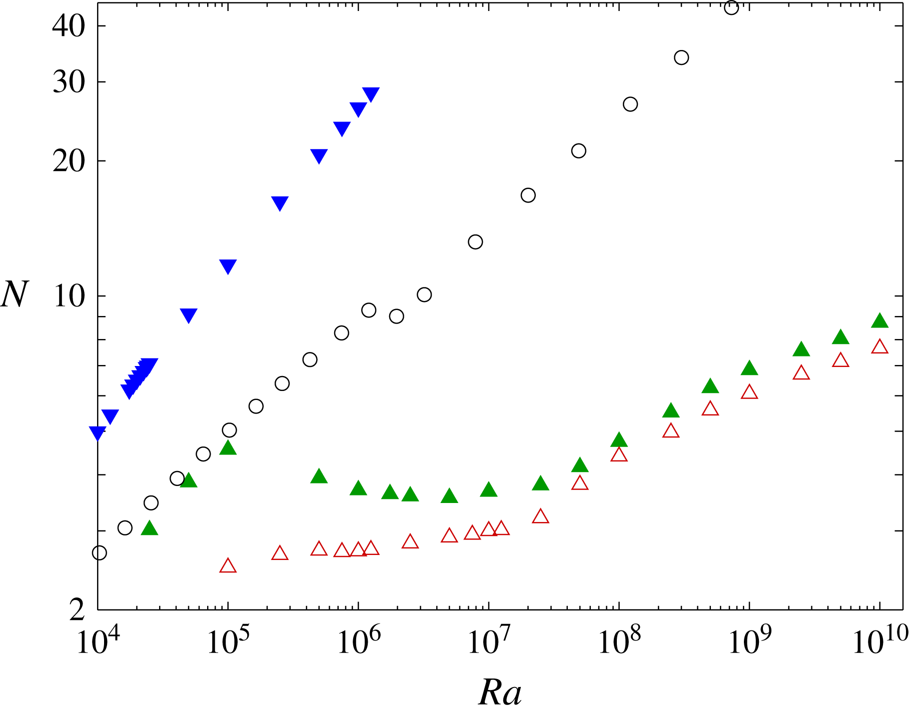
Mean Nusselt numbers,
 $N$
, for various Rayleigh numbers with
 $\mathit{Pr}=1$
. For
 $A=2$
, bursting shearing convection (▴) and non-shearing convection (▾) are represented. For
 $A=1$
, only bursting shearing convection (▵) is represented. Nusselt numbers computed by Johnston & Doering (Reference Johnston and Doering2009) for no-slip boundaries and
 $A=2$
are also shown (○).

B.2. Effects of boundary conditions and aspect ratio with
$\mathit{Pr}=1$

Figure 12 shows Nusselt numbers of RB convection under several different conditions, all with
 $\mathit{Pr}=1$
. Bursting shearing states shown in the figure (▴) appear also in figure 10 alongside shearing states for other Prandtl numbers. Here, they are compared to non-shearing states (▿) under the same conditions. Nusselt numbers are larger and grow much faster with
 $\mathit{Ra}$
in the non-shearing case, as is also true at other Prandtl numbers (cf. figure 4). When the horizontal period is halved to
 $A=1$
, the Nusselt numbers of shearing convection (▵) become monotonic in
 $\mathit{Ra}$
.
The monotonic growth of
 $N$
that we find with
 $(A,\mathit{Pr})=(1,1)$
is consistent with the simulations of Garcia et al. (Reference Garcia, Bian, Paulsen, Benkadda and Rypdal2003), where
 $A$
and
 $\mathit{Pr}$
were the same, but the heat flux, rather than the temperature, was fixed at the top boundary. To see this, we must reformulate the findings of Garcia et al. (Reference Garcia, Bian, Paulsen, Benkadda and Rypdal2003) in terms of
 $N$
and
 $\mathit{Ra}$
. They report a fit equivalent to
 $\langle T\rangle ^{t}\propto R^{-0.08}$
, where
 $R$
is a Rayleigh number defined using the temperature difference between the boundaries in the static state. If we define
 $N$
and
 $\mathit{Ra}$
using the temperature difference between the boundaries in the developed convection, as is suited to comparing flows with different thermal boundary conditions (Otero et al.
Reference Otero, Wittenberg, Worthing and Doering2002; Johnston & Doering Reference Johnston and Doering2009; Wittenberg Reference Wittenberg2010), then the Nusselt number is the inverse of the temperature difference between the boundaries, and
 $\mathit{Ra}\propto R/N$
. Since this temperature difference scales like
 $\langle T\rangle ^{t}$
at large Rayleigh numbers,
 $N\propto 1/\langle T\rangle ^{t}$
, and
 $\mathit{Ra}\propto R\langle T\rangle ^{t}$
. In these terms, the findings of Garcia et al. are that
 $N\propto Ra^{0.087}$
. That is,
 $N$
increases slowly but monotonically with
 $\mathit{Ra}$
, much as in our simulations.
When no-slip, rather than free-slip, conditions are imposed at the boundaries, only non-shearing states have been reported when
 $(A,\mathit{Pr})=(2,1)$
. The Nusselt numbers of these non-shearing states (○) are smaller than those of non-shearing convection between free-slip boundaries (▾) but larger than those of shearing convection between free-slip boundaries (▴).