





Introduction
High-frequency communication and radar systems demand efficient, low-loss transmission lines capable of handling high power levels. Conventional rectangular waveguides are widely used in such applications due to their superior power handling and low-loss characteristics. However, the requirement for metal-to-metal contact in traditional waveguide assemblies often increases complexity and reduces long-term reliability.
Gap waveguide technology (GWT), proposed as an alternative to conventional designs, enables contactless wave propagation by introducing periodic pin structures between parallel conducting plates. These periodic structures create a stopband that suppresses unwanted modes, allowing electromagnetic waves to propagate only in desired paths [Reference Kildal, Alfonso, Valero-Nogueira and Rajo-Iglesias1–Reference Cui, Chen, Sun and He5]. GWT has found applications in a variety of high-frequency components, such as filters, antennas, and couplers, as well as in packaging techniques [Reference Alos, Zaman and Kildal6–Reference Ahmadi and Banai13], where ease of fabrication and assembly without electrical contact is particularly advantageous.
Waveguide switches are essential for systems that require signal routing, including radar front ends, satellite payloads, and RF test systems. Mechanical waveguide switches, in particular, are favored for high-power applications due to their robustness, low insertion loss, and high isolation. Although several studies have explored the use of GWT in switch designs [Reference Farahbakhsh14–Reference Tayebpour, Ahmadi, Fallahzadeh, Shekoo and Torabi19], they are typically limited in configurability, integration with actuation systems, or power handling capabilities.
This work presents the design and implementation of a novel mechanical waveguide switch operating in the X-band (8.2–12.4 GHz) that utilizes GWT for contactless, low-loss operation. The switch supports both double-pole double-throw (DPDT) and single-pole double-throw (SPDT) configurations and can withstand up to 100 kW of peak power. It consists of a rotatable inner cylinder enclosed in a stationary outer cube, with a non-contact interface that leverages GWT principles. Additionally, a compact rotary actuator mechanism is developed and integrated into the system, enabling reliable switching within 50 ms.
The main contribution of this work is the development of a fully integrated high-power waveguide switch that combines GWT with a custom-designed rotary actuator. The design simplifies manufacturing through its contactless interface, enhances electrical performance through optimized geometric parameters, and ensures safe operation at high power levels via detailed RF breakdown simulations. The switch’s performance is validated by electromagnetic and mechanical simulations and experimental measurements, with strong agreement across the full X-band.
The gap waveguide technology
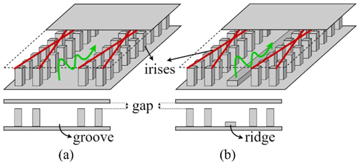
The concept of a gap waveguide is based on controlling the propagation of an electromagnetic wave in a waveguide with parallel plates, allowing it to propagate only in desired directions, using the fundamentals of boundary conditions and canonical surfaces. Pins are periodically placed on only one of the plates with a gap between the pins and the other plate (Fig. 1). In this way, the signal is transmitted between two plates that are not in contact with each other. This enables control of signal transmission and limits unwanted signal propagation between two contactless plates, making it easier to manufacture and combine the plates than their conventional counterparts.
Gap waveguide geometries and signal propagation. (a) Groove gap waveguide. (b) Ridge gap waveguide.

Figure 1 shows two GWT configurations and their corresponding signal transmission paths. In GWT, pins placed on one of the metal plates can serve as a bed of nails, but they can also be designed in different periodic shapes [Reference Silveirinha, Fernandes and Costa20, Reference Rajo-Iglesias and Kildal21]. Periodic structures create a high impedance for surface waves. The wave cannot propagate in this region. To create the stopband for the wave, the gap between the plate and the pins must be smaller than the signal’s quarter wavelength (λ/4). To create a propagation path for the waves, the space between the pins is left empty (Fig. 1(a)) or a metal plate is placed (Fig. 1(b)). These are called the groove-gap waveguide and the ridge-gap waveguide, respectively [Reference Kildal22, Reference Kildal, Zaman, Rajo-Iglesias, Alfonso and Valero-Nogueria23]. The signal travels in the space between the plates or the space between the ridge and the other plate.
Switch design
The waveguide switch consists of an inner cylinder and an outer cube, manufactured separately. The inner cylinder is placed inside the outer cube using the shrink-fit method. The electromagnetic simulations of the waveguide switch were performed using CST Studio Suite (Dassault Systèmes) [Reference Systèmes24].
The outer cube
Four WR90 ports are placed on the side surfaces of the stationary outer cube. There is a 90° angle between the ports on the horizontal axis. The outer cube is designed as a shell for the motor, actuating mechanism, and switch. The outer cube is connected to the inner cylinder via bearings at the top and bottom. Inside the outer cube, there is a cavity in which the inner cylinder is positioned and rotates. The radius of this cavity is larger than the radius of the inner cylinder, so that the inner cylinder can rotate easily inside the outer cylinder. Ports on the outer cube transmit the signal to the switch. Switching occurs when the inner cylinder is rotated 90° while the outer cylinder remains stationary. For switching, the motor located at the top of the outer cube drives the actuating mechanism, which rotates the inner cylinder.
The design and fabricated models for the outer cube structure are given in Fig. 2.
Outer structure. (a) Design model. (b) Fabricated model.

The inner cylinder
The inner cylinder contains two signal transmission paths, each consisting of a 90° bend WR90 waveguide. Rotating the inner cylinder by 90° changes the ports to which the waveguides are connected, and switching takes place. The rotation of the inner cylinder is provided by the bearings located at the top and bottom. The bends and bearings in the inner cylinder are shown in Fig. 3. Figure 3(a)–(c) shows the design models, while Fig. 3(d)–(f) shows the production models.
Inner cylinder. (a–c) Design model. (d–f) Production model.

Figure 3 Long description
A six-panel figure comparing CAD models and manufactured parts of an inner cylinder assembly. The first three panels illustrate design models, while the last three show production models. The image A depicts a CAD cutaway rendering of a cylindrical inner part within a square outer block, featuring a bearing at the top. Multiple vertical channels are visible around the cylinder. The image B shows another CAD cutaway rendering with the top plate removed, revealing a pin near the upper rim and repeated vertical channels. The image C presents a simplified schematic of channel paths with U-shaped bends, labeled as bend and radial tick marks around the perimeter. The image D is a photograph of the manufactured square metal block with a circular top plate and fasteners. The image E shows a photograph of the manufactured part with visible vertical channels around the inner cylinder. The image F is a close-up photograph of a circular machined component with curved channel openings forming U-shaped paths and radial fins around the edge. The assembly is designed to facilitate signal transmission through waveguides, with the bearing allowing rotation and the pin and bend contributing to the structural and functional integrity of the system.
A DPDT waveguide switch is one in which two inputs and two outputs are controlled. If one of the ports is set to a blank wall, the switch operates in SPDT mode. The switching configurations for DPDT and SPDT are shown in Fig. 4.
Switching configurations for DPDT and SPDT.

The signal that reaches the switch via the port on the outer cube must travel through the bend structure on the inner cylinder. However, the inner cylinder and the outer cube are separate parts, with a gap between them. The GWT is used to prevent the signal from leaking through this gap. The square pin arrays on the inner cylinder’s side surface are designed to be periodic. The pins create a high impedance on the inner cylinder’s side surface. Thus, the signal continues to travel along the bend instead of leaking through the gap between the outer cube and the inner cylinder. The design parameters that affect the leakage amount are the gap size between the inner cylinder and the outer cube, g, the pin sizes (width, wp, and height, hp), the gap between the pins (gp), and the radii (ri and ro) of the inner cylinder as depicted in Fig. 5.
Dimensions of the parts of the inner cylinder.

Figure 5 Long description
Two sub images are shown, a main dimensioned cross section and a detail view connected by two diagonal guide lines. The main view shows a square outer boundary containing a circular inner cylinder, with a vertical rectangular bar passing through the center of the circle and extending to the top and bottom edges of the square. Around the circular boundary, four curved ring like segments are drawn, separated by the central vertical bar and by gaps between the curved segments. Several dimension arrows and leader lines point to features on the curved segments and the circular boundary. Text labels include w subscript p beside a dimension arrow spanning a short straight distance on one curved segment, h subscript p beside a dimension arrow spanning a short radial distance on a curved segment, r subscript i beside a leader pointing to an inner circular arc and r subscript o beside a leader pointing to an outer circular arc. A small circled region is marked on one curved segment near the right side of the main view and two diagonal lines extend from that circled region to the detail view. The detail view shows two curved boundaries forming a narrow wedge shaped region, with a short dimension line across the gap between the two boundaries labeled g. No numeric values or measurement units are shown.
In a waveguide switch, the insertion loss between two ports with a bend connection is expected to be as low as possible (close to zero). On the other hand, return loss at each input port is expected to be high.
The bend radius (rb) affects the return loss. Figure 6 shows a plot of the simulated return loss for only a change in the bend radius values. In this design, the bend radius where the return loss is the best is 8.3 mm.
Return loss for different bend radii.

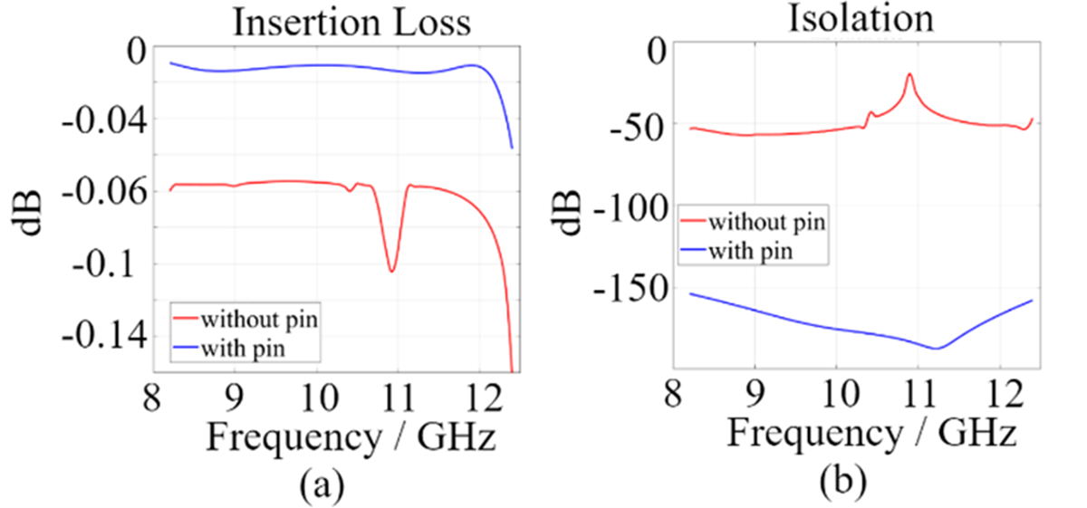
In a waveguide switch, the isolation between the ports that are not connected via a waveguide is expected to be high. Pins provide isolation by preventing wave leakage through the gap between the inner and outer structures. Figure 7 shows the effect of the design with and without pins (all pins are removed from the structure) on insertion loss and isolation. When the pins on the structure are removed, the insertion loss increases from a maximum of 0.05–0.15 dB. Likewise, the isolation value decreases from a minimum of 150–20 dB. The peak observed when the pins are removed is caused by electromagnetic leakage into the gap between the inner cylinder and the outer cube, where the gap region behaves as a resonant cavity at that frequency.
(a) Insertion and (b) isolation with pin and without pin.

Figure 7 Long description
A line graph titled, Insertion Loss. The horizontal axis is labeled, Frequency slash GHz, with tick labels 8, 9, 10, 11, 12. The vertical axis is labeled, decibel, with tick labels 0, minus 0.02, minus 0.04, minus 0.06, minus 0.08, minus 0.1, minus 0.12, minus 0.14. A legend lists two series: without pin and with pin. The without pin curve stays near minus 0.06 decibel from 8 to about 10.5 gigahertz, then drops to about minus 0.14 decibel near 11 gigahertz and rises back toward about minus 0.06 decibel by 12 gigahertz. The with pin curve stays close to 0 decibel from 8 to about 11.5 gigahertz, then drops to about minus 0.02 decibel near 12 gigahertz. The image B showing a line graph titled, Isolation. The horizontal axis is labeled, Frequency slash GHz, with tick labels 8, 9, 10, 11, 12. The vertical axis is labeled, decibel, with tick labels 0, minus 50, minus 100, minus 150. A legend lists two series: without pin and with pin. The without pin curve is near minus 50 decibel from 8 to 12 gigahertz, with a narrow peak rising toward about minus 20 decibel around 10.5 gigahertz. The with pin curve is near minus 150 decibel from 8 to 12 gigahertz, with a shallow dip below minus 150 decibel around 10.5 gigahertz.
Insertion loss, return loss, and isolation for different gap values.

Figure 8 Long description
Return Loss line graph. Horizontal axis label, Frequency slash GHz, with tick labels 8, 9, 10, 11, 12. Vertical axis label, dB, with tick labels negative 80, negative 60, negative 40, negative 20. Legend entries, g equals 0.02 mm, g equals 0.06 mm, g equals 0.10 mm, g equals 0.14 mm. The four curves show multiple dips across 8 to 12 GHz, with the deepest dip reaching near negative 80 dB. Several dips occur around the tick marks near 9, 10, 11 and 12 GHz, with curve values between about negative 20 dB and negative 60 dB between dips. Insertion Loss line graph. Horizontal axis label, Frequency slash GHz, with tick labels 8, 9, 10, 11, 12. Vertical axis label, dB, with tick labels 0, negative 0.02, negative 0.04, negative 0.06, negative 0.08. Legend entries, g equals 0.02 mm, g equals 0.06 mm, g equals 0.10 mm, g equals 0.14 mm. Three curves stay close to 0 dB across most of 8 to 12 GHz, with small ripples around negative 0.02 dB to negative 0.04 dB. One curve drops sharply near the high end of the frequency range, reaching close to negative 0.08 dB. Isolation line graph. Horizontal axis label, Frequency slash GHz, with tick labels 8, 9, 10, 11, 12. Vertical axis label, dB, with tick labels negative 220, negative 180, negative 140, negative 100. Legend entries, g equals 0.02 mm, g equals 0.06 mm, g equals 0.10 mm, g equals 0.14 mm. The four curves slope upward from 8 to 12 GHz. One curve stays much lower than the others, near negative 200 dB to negative 220 dB with small ripples. The other three curves span roughly negative 100 dB to negative 180 dB, with separation between them across the band. Across the three graphs, the same four gap labels are compared over the same frequency range, with return loss showing repeated notches, insertion loss staying near 0 dB except for one sharp drop near the upper end and isolation showing separated curves that rise toward less negative values as frequency increases.
The gap between the outer cube and the rotating inner cylinder is a parameter that directly affects all results. A small gap improves return loss, insertion loss, and isolation. However, the inner cylinder structure needs space to rotate inside the outer cube. It is important to choose the gap value that provides the best results and facilitates production and integration. The scattering parameters simulated by varying the gap between the outer cube and the inner cylinder are given in Fig. 8. In this study, the electrical targets of the design are as follows: insertion loss <0.05 dB, return loss >30 dB, and isolation >80 dB. For mechanical constraints, the manufacturing tolerance should be on the order of 0.02 mm. A gap of 0.04 mm between the inner cylinder and the outer cube is required for a shrink fit of the inner cylinder into the cavity inside the outer cube. Therefore, the optimum gap value of 0.06 mm is chosen for good electrical performance of the switch and ease of fabrication and assembly. Unlike [Reference Tayebpour, Ahmadi, Fallahzadeh, Shekoo and Torabi19], the gap-waveguide pin structure in this work is directly integrated along the cylindrical rotor interface, where leakage is most critical during rotation. This configuration enables stronger field confinement and is a key factor in achieving the reported wideband and high-isolation performance.
Based on the simulations, the design parameters for the waveguide switch are given in Table 1.
Design parameters of the waveguide switch

Measurement
The designed waveguide switch is manufactured from aluminum. The inner cylinder was produced in two separate parts and assembled with bolts. Bearings are added to the top and bottom of the inner cylinder to ensure rotation. The inner cylinder is positioned in the cavity of the outer cube by shrink fitting. The outer layer was produced in three separate parts: the outer cube, the actuating mechanism, and the cover. These parts are connected with bolts.
The scattering parameters of the mechanical waveguide switch are measured with a two-port vector network analyzer. While measuring the scattering parameters between two ports, the other ports were terminated with a matched load. The measurement setup is shown in Fig. 9.
Measurement setup of the waveguide switch.

The scattering parameters of the designed and fabricated waveguide switch are given in Table 2 and Fig. 10. The scattering parameter results of the designed switch are in agreement with the measurement results of the manufactured switch.
Scattering parameters for simulation and measurement

Scattering parameters for simulation and measurement: (a) Return loss. (b) Insertion loss. (c) Isolation.

Figure 10 Long description
Return Loss. The x-axis is labeled, Frequency slash GHz, with ticks at 8, 9, 10, 11 and 12. The y-axis is labeled, decibel, with ticks at minus 30, minus 40, minus 50, minus 60 and minus 70. A legend shows two series: Meas. and Sim. The Meas. curve stays near minus 35 to minus 40 decibel with small ripples and has two deep notches: one near 9 gigahertz reaching about minus 70 decibel and another near 11 gigahertz reaching about minus 70 decibel. The Sim. curve is smoother and stays around minus 35 to minus 40 decibel, with shallower dips around the same frequencies. Insertion Loss. The x-axis is labeled, Frequency slash GHz, with ticks at 8, 9, 10, 11 and 12. The y-axis is labeled, decibel, with ticks at 0, minus 0.02, minus 0.04, minus 0.06 and minus 0.08. A legend shows two series: Meas. and Sim. The Meas. curve varies between about minus 0.02 and about minus 0.08 decibel, with several troughs: near 9 gigahertz around minus 0.08 decibel, near 10 gigahertz around minus 0.07 decibel and near 12 gigahertz around minus 0.08 decibel. The Sim. curve stays close to 0 decibel with small variation. Isolation. The x-axis is labeled, Frequency slash GHz, with ticks at 8, 9, 10, 11 and 12. The y-axis is labeled, decibel, with ticks at minus 90, minus 110, minus 130, minus 150 and minus 170. A legend shows two series: Meas. and Sim. The Meas. curve lies between about minus 100 and minus 120 decibel, rising toward about minus 100 decibel near 11 gigahertz and then dropping again toward 12 gigahertz. The Sim. curve is much lower, around minus 150 to minus 170 decibel, with a broad minimum near 11 gigahertz close to minus 170 decibel.
Table 3 compares the proposed switch with previously reported waveguide switch designs. As shown in the table, the proposed switch provides the widest bandwidth, covering the entire X-band. While the insertion loss (IL) performance is comparable to that of existing designs, the proposed structure achieves improved return loss (RL) and isolation (Iso.). In particular, the proposed design provides a return loss above 30 dB and an isolation above 90 dB, whereas previously reported designs typically exhibit return loss values below 20 dB and isolation levels below 60 dB [Reference Ruiz-Cruz, Fahmi and Mansour16, Reference Tayebpour, Ahmadi, Fallahzadeh, Shekoo and Torabi19]. These results demonstrate the improved RF performance achieved by the proposed switch. It should also be noted that, unlike the design presented in [Reference Tayebpour, Ahmadi, Fallahzadeh, Shekoo and Torabi19], the proposed switch employs a gap-waveguide-based structure with a dedicated actuator mechanism, enabling improved RF performance and wideband operation.
RF performance comparison between the proposed switch and previously reported waveguide switches

RF breakdown analysis
A system used in high-frequency, high-power applications is expected to transmit a high-power signal. The inability of the system to withstand a high-power signal, which can damage the structure and prevent transmission, is called RF breakdown or electrical breakdown. RF breakdown can be explained by corona discharge and multipacting.
The corona effect occurs naturally in high-power applications because air, which contains many free electrons and ions under normal conditions, is not a perfect insulator. When an electric field passes through the air between two conductors, electrons on the surface of the conductor are ejected if they reach sufficient energy. Under the influence of the electric field, free ions and electrons in the air are exposed to a force. As a result, ions and free electrons accelerate. During their movement, charged particles collide with each other and with slow-moving uncharged molecules. Thus, the number of charged particles increases rapidly. If the electric field strength between electrons is strong enough, the interactions between electrons become non-negligible. The strength of the electric field causes electrons to break away from the conductors and the air surrounding the conductors to dissociate into ions. This makes the air conductive, leading to arcing between the conductors [Reference Veldhuizen and Rutgers25].
Electron multipacting is a phenomenon in vacuum tubes and waveguides to which RF and high-power signals are applied, in which, under certain conditions, the emission of secondary electrons in resonance with an electric field leads to exponential electron multipacting, damaging or even destroying the RF device. This is especially important to consider in high-power space applications.
When electrons, accelerated by an electric field in a cavity, hit the surface of this cavity, they eject electrons from the surface. The accelerated electrons are called “primary electrons,” and the electrons removed from the surface by the primary electrons are called “secondary electrons.” Depending on the impact, energy, and angle of the primary electron on a surface, the cavity can release one or more secondary electrons into the vacuum. These electrons can then be accelerated by electric fields and hit the same or another surface. If the energy and frequency of the electric field increase, the number of electrons ejected increases, leading to a multipacting effect [Reference Sounas26]. When the number of free electrons in the medium reaches a non-negligible level, the medium becomes conductive. In prolonged electron multipacting, the structure can be physically damaged. It is therefore important to perform high-power testing of components.
Multipacting depends on the material used in the system. Secondary electron emission (SEE) is a high-power parameter that varies with material. The Vaughan and Furman models are the two main models for SEE-type materials.
In this study, multipactor analysis is used as a design verification tool to evaluate the switch’s high-power endurance rather than performing a detailed parametric multipactor investigation. Analysis is performed using the particle-in-cell template in the Particle Studio package within the commercial CST program to assess the switch’s high-power endurance. For the multipacting simulation, the switch’s building material is selected as “SEE-Aluminum,” which exhibits SEE. To analyze the effect of primary electrons on the structure, three distinct primary-electron interfaces are defined along the electric-field transmission path. As shown in Fig. 11, 1000 electrons are assigned to each electron interface, for a total of 3000 electrons.
Electron interfaces on the transmission of the switch.

In total, 100 kW of power is applied to the switch for 100 ns. Primary electrons hit the surfaces at power levels below 100 kW. If the structure can withstand this power, no multipacting occurs, and the number of electrons decreases over time. The sum of the primary and secondary electron numbers is called particle number, and the particle number versus time is given in Fig. 12(a). The electrons on the structure at the end of 100 ns are also shown in Fig. 12(b).
The number of primary and secondary electrons (a) versus time (b) on the structure (100 kW).

As seen in Fig. 12, the number of electrons inside the switch decreases over time. Based on the simulations, it was concluded that the structure can withstand the desired power of 100 kW and that there is no RF breakdown within it. The structure can withstand 100 kW; however, analyses were performed to determine the power at which the structure experiences RF breakdown. The analysis determined that the structure cannot withstand 125 kW of power. The particle number versus time for 125 kW is given in Fig. 13(a). The electrons on the structure at the end of 90 ns are also shown in Fig. 13(b).
The number of primary and secondary electrons (a) versus time (b) on the structure (125 kW).

As shown in Fig. 13, the number of particles increased rapidly over the first 90 ns. That is, electron multipacting occurred on the switch transmission path. The switch cannot withstand 125 kW power.
Actuating mechanism
In the waveguide switch used in high-power communication systems, rotary movement between the RF transmission lines is achieved via a rotary actuator with an electromechanical operating mechanism. The actuator analysis presented in this section focuses on the design methodology and the estimation of the required torque and switching time for the proposed waveguide switch. The actuator mechanism simulations were carried out using COMSOL Multiphysics (COMSOL AB). In addition, the mechanical parameters of the rotating structure, such as the moment of inertia, were obtained using SolidWorks [27]. Providing high torque in milliseconds, it typically has a structure that includes permanent magnets, coil, outer and inner housings, and other mechanical fasteners [Reference Microwave28]. The limits of the developed waveguide switch actuator mechanism are given in Table 4.
Actuator design limits

Table 4 Long description
Actuator design limits are summarized for rotation time, operating current, and operating voltage. Rotation time is 50 milliseconds. The actuator current limit is 0.9 amps, and the actuator voltage limit is 28 volts. The table lists single values only, so it does not indicate variation, tolerances, or test conditions. No comparisons across models or operating modes are provided, so these values should be treated as stated limits rather than performance across a range.
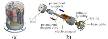
The actuator mechanism is designed to be failsafe, returning to its starting position when the power is cut off. The transparent appearance and flat structure of the integrated actuator mechanism are shown in Fig. 14.
The integrated actuator mechanism (a) with the transparent view and (b) with flat-looking structure.

Figure 14 Long description
Integrated actuator mechanism with a transparent view, revealing internal components. Exploded view of the actuator mechanism with labeled parts. Starting from the left, the front unit is followed by permanent magnets, which are connected to a permanent magnet core. An electromagnet is positioned next to the core. To the right, the actuator housing is shown, followed by a spring and a base plate. Each component is clearly labeled to indicate its position and function within the mechanism.
The actuator’s rotation is enabled by the magnetic circuit formed by the coil, permanent magnets, and high-permeability materials. A core material with high magnetic permeability holds the permanent magnets together, and the rotation torque is transferred to the waveguide via this shaft. There is a coil and two permanent magnets inside the structure. The main magnetic circuit is completed through these elements. In addition, a spiral spring provides the structure’s failsafe feature, along with a spring guide that surrounds it. The remaining elements were selected based on the need for magnetic permeability, the BH curve for completing the magnetic circuit, and the mechanical fixation of the structure [Reference Microwave28]. The materials for the actuator components are defined in Table 5.
Actuator components with their materials

Considering the specifications of the waveguide switch, the amount of torque needed to perform the rotation movement in the desired time is obtained with a formulation [29]:
 \begin{equation}\tau = I*\omega = I*\frac{{2\theta }}{{{t^2}}}\end{equation}
where  $\tau $ is torque,
 $I$ is inertia,
 $\omega $ is angular velocity,
 $\theta $ is rotation angle, and
 $t$ is rotation time. τ of ∼6.27 Ncm is required to switch a waveguide with
 $I$ of 49,918
 $gm{m^2}$ (obtained from SolidWorks) under 50 ms in theoretical approach.
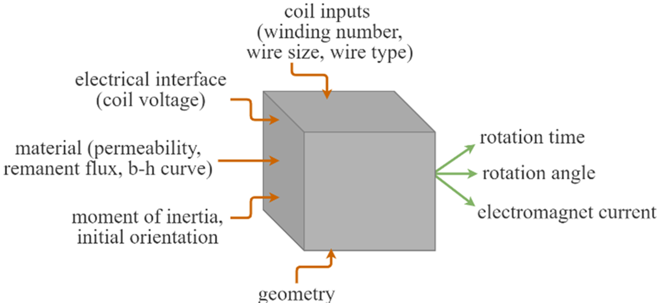
 $\theta $ is obtained from the derivative of the angular velocity. Moreover, actuator simulation was primarily performed by defining the number of coil windings, the conductor wire diameter, the BH curves of the hard and soft magnetic materials used, the residual magnetization, the magnetic permeability, and the coil voltage. The simulation parametric context structure is given by the black-box model in Fig. 15. The simulation results are evaluated with respect to the electromagnet current, rotation time, and rotation angle.
Black-box model for parametric relation of the actuator simulation.

The simulations are carried out in COMSOL Multiphysics. COMSOL is a software that simulates structures in applications such as acoustics, electromagnetics, chemical reactions, mechanics, fluid flow, and heat transfer by solving Maxwell’s equations. In this study, to obtain the best results for the actuator mechanism, several designs, including double- and single-coil and inner-outer rotor configurations, are evaluated. According to the simulation results, the best solution to achieve the failsafe mode is the single-coil, inner-rotor drive mechanism.
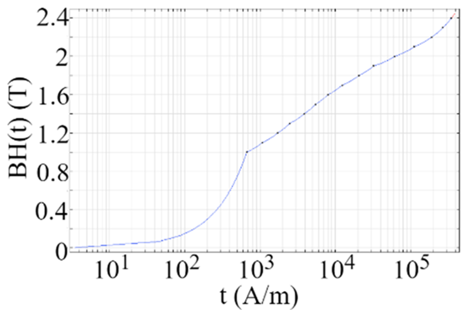
Figure 16 shows the BH graph for soft iron, the most commonly used material for magnetic circuit design in this kind of application. Since it requires a small A/m to reach a high magnetic field, compared to other high-permeability materials like nickel alloys or low-carbon steel. In this actuator, the electromagnet core and housing are made of soft iron.
BH graph for soft iron.

The magnetic field required to initiate rotation is related to the number of windings and the coil current. The coil is designed with the wire depending on the current capacity and coil core. Figure 17(a) shows the current through the wires over time for different winding numbers. Regardless of the number of windings and wire types, the volume the coil will occupy is the same in each scenario. The purpose of this analysis is to determine a suitable winding number regarding wire current capacity. American wire gauge (AWG) is a standard that numbers wires by size. After many attempts with different AWG wire sizes, AWG 37 wire, with a maximum current capacity of 22 mA, is used in this design. As seen in Fig. 17(b), except for 10,000 winding numbers, the other winding numbers exceed the maximum current capacity while the actuator reaches 90° of rotation. In the graph, 10,000 windings of wire draw a current of ±20 mA. A 0.8 T magnet is used in this simulation.
Time-dependent (a) coil current and (b) rotation angle of the actuator for different coil winding numbers (t).

Figure 17 Long description
A line graph titled, coil current (A). The horizontal axis is time (ms), ranging from 0 to 24. The vertical axis is coil current (A), ranging from negative 0.02 to 0.02. A legend lists t equals 6000, t equals 8000, t equals 10000, t equals 12000 and t equals 14000. Five lines are plotted. Each line starts near 0.02 at time 0, decreases to a minimum near time 12, rises to a local maximum near time 18, then decreases again toward time 24. The image B showing a line graph titled, rotation angle (degree). The horizontal axis is time (ms), ranging from 0 to 24. The vertical axis is rotation angle (degree), ranging from 10 to 180. A legend lists t equals 6000, t equals 8000, t equals 10000, t equals 12000 and t equals 14000. Five lines are plotted. Each line increases from about 10 at time 0 to about 180 at time 24, with a change in slope around time 12.
The remaining part of the analysis was performed with a winding number of 10,000. The second part of the study was determined by the residual magnetization parametric approach applied to the selected permanent magnet in the simulation to select the permanent magnet type. Accordingly, a 0.8 T residual magnetized permanent magnet offers the best solution in terms of rotation time and coil current.
As shown in Fig. 18(b), as the magnet’s remanent flux increases, the time required for a 90° rotation decreases. Figure 18(a) shows the current drawn by the coil wire as a function of different remanent flux values. The selected AWG 37 wire can withstand a maximum current of 20 mA. When Fig. 18(a) and (b) are analyzed together, a 0.8 T magnet is chosen so that the current passing through the wire is less than 20 mA and the switching time is close to 20 ms.
Time-dependent (a) coil current and (b) rotation angle of the actuator for different permanent magnet fluxes (B).

Figure 18 Long description
Two multi-line graphs. The first graph shows coil current in amperes over time in milliseconds, with the x-axis labeled ′time (ms)′ ranging from 0 to 24 milliseconds and the y-axis labeled ′coil current (A)′ ranging from negative 0.02 to positive 0.02 amperes. Four lines represent different magnet flux values: B equals 0.5 T, B equals 0.6 T, B equals 0.7 T and B equals 0.9 T. The lines are visually distinguished by different styles, as indicated in the legend. The graph demonstrates that higher magnet flux values tend to result in larger current magnitudes and earlier peaks. The second graph displays rotation angle in degrees over time, with the x-axis labeled ′time (ms)′ and the y-axis labeled ′rotation angle (°)′ ranging from 0 to 130 degrees. It includes the same four lines for magnet flux values. The graph shows that higher flux values lead to faster and higher rotation angles over time. Major peaks and troughs occur at different times for each flux value, with B equals 0.9 T showing the fastest increase in rotation angle. The purpose of these graphs is to illustrate the effect of increasing magnet flux on current waveform and rotation angle growth.
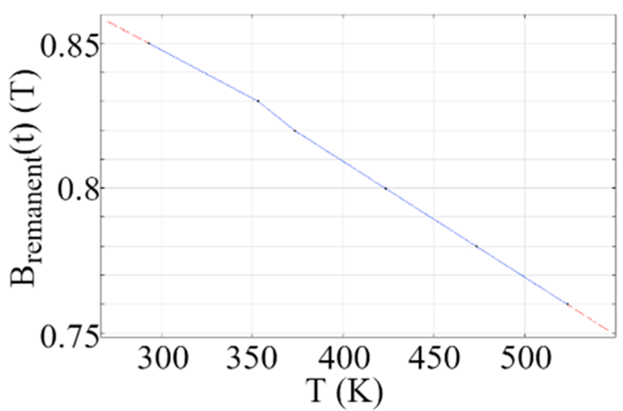
The actuator design in this study uses a Samarium Cobalt magnet (YX-16) because of its superior temperature resistance. Figure 19 shows the temperature-related residual flux characteristic of this magnet.
Temperature-related remanent flux characteristic for Samarium Cobalt YX-16.

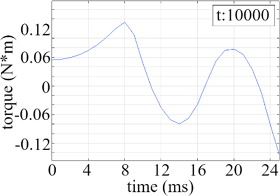
The torque amounts depending on time are given in Fig. 20 with the latest design structure decided. The graph shows that 14 Ncm values are reached. This value meets the 6.4 Ncm value required for switching as calculated in (1).
Final design decisions are given in Table 6 for the rotary actuator of the waveguide switch.
Time-dependent torque of the actuator for 10,000 turns.

Final parameters of the actuator mechanism

Conclusion
Compared to previously reported waveguide switch structures, the proposed design offers a unique combination of GWT and integrated actuation, enabling contactless high-power operation with faster switching time and improved electrical performance. This paper presents the design of DPDT and SPDT mechanical waveguide switches for high-power X-band applications. The switch structure consists of a rotatable inner cylinder and a fixed outer cube, with no physical contact between them, ensuring ease of assembly and improved durability. The design can withstand up to 100 kW of peak power. The fabricated prototype has been tested and shows strong agreement with the simulation results, achieving a return loss greater than 30 dB, an insertion loss below 0.1 dB, and an isolation above 90 dB. The switching mechanism is controlled by a custom-designed rotary actuator, and the actuator is designed to achieve a switching time below 50 ms when operated under a 28 V supply.
Funding statement
This study was supported by TUBITAK under project number 119C032.
Competing interests
The authors declare none.

Merve Güvenç received the B.Sc. degree in electrical and electronics engineering from Yeditepe University, Istanbul, Turkey, in 2020. She started her Ph.D. after completing her M.Sc. at Yeditepe University in 2020. She has been working as an RF design engineer at Profen Technologies since 2020. Her current research interests include computational electromagnetics, RCS measurements, electromagnetic analysis, design of high-power antennas, and communication systems components.

Çağlar Konak was born in Istanbul, Turkey, in 1991. He received both the B.Sc. and M.Sc. degrees in physics from Middle East Technical University, Ankara, Turkey, in 2015 and 2019, respectively. Between 2015 and 2019, he participated in the AMS Collaboration at CERN, focusing on understanding the space radiation environment through the proton spectrum and the effects of solar modulation. He is interested in finite element analysis, precision cleaning and packaging, beam and material interactions, vacuum tube conditioning setups, and electromagnetic actuator mechanisms for communication systems.

İsmail Şişman was born in Istanbul. He received his bachelor’s and master’s degrees in electronics and communication engineering from Haliç University in 2009 and 2011, respectively. He completed his Ph.D. degree in electrical and electronics engineering at Yeditepe University. He worked as a Research Assistant at the Electrical and Electronics Engineering Department of Haliç University between 2009 and 2012, and as a Research Assistant at Yeditepe University between 2012 and 2017. Since 2017, he has been working as RF Group Manager at the R&D Centre of PROFEN Technologies, a company operating in the satellite communication sector.

A. Arif Ergin was born in Ankara, Turkey, in 1970. He received the B.Sc. degree in electrical and electronics engineering from the Middle East Technical University, Ankara, Turkey, in 1992, and the M.Sc. and Ph.D. degrees in electrical and computer engineering from the University of Illinois at Urbana-Champaign, Urbana, in 1995 and 2000, respectively. Between 2000 and 2016, he was with the Electronics Engineering Department, Gebze Technical University. He also assumed part-time positions on various projects in TÜBITAK. Between 2014 and 2015, he served as the President of TÜBİTAK Informatics and Information Security Research Center. Between 2015 and 2018, he was the President of TÜBİTAK. Since 2024, he has been with the Bahçeşehir University, Electric and Electronics Engineering Department. He is interested in numerical analysis, simulation, and measurement of electromagnetic wave phenomena.









 Open access

