1 Introduction
Our concern is with the inviscid limit of stability for unidirectional flow
 $U$
varying in two cross-streamwise directions
 $y$
and
 $z$
. The inviscid stability has long been studied for a more restricted form of background flow
 $U(y)$
since the early days of modern theoretical fluid dynamics. Many standard fluid dynamics textbooks devote a section to analysing the Rayleigh equation
 $$\begin{eqnarray}\displaystyle v_{yy}-\unicode[STIX]{x1D6FC}^{2}v-\frac{U_{yy}}{U-c}v=0, & & \displaystyle\end{eqnarray}$$
deduced from the two-dimensional Euler equations linearised around
 $U(y)$
. For a given perturbation wavenumber
 $\unicode[STIX]{x1D6FC}$
, the above equation and the boundary conditions (usually impermeability conditions are used on the walls) constitute a linear eigenvalue problem for a complex phase speed
 $c$
. When
 $c$
is purely real, namely when the (Fourier-transformed) perturbation velocity
 $v$
is neutral, the equation has a regular singular point, whose nature is well understood (Lin Reference Lin1945, Reference Lin1955). Otherwise, a perturbation growing in time should exist, but this is possible only when
 $U(y)$
has at least one inflection point; this is the famous Rayleigh’s inflection point theorem and can be obtained by multiplying
 $v^{\ast }$
, the complex conjugate of
 $v$
, with (1.1) and integrating it over the flow domain.
The generalisation of the above classical inviscid stability result to
 $U(y,z)$
is of enormous importance in describing a wide range of real-world flows such as those through non-circular pipes or over corrugated walls. However, there have been surprisingly few analytic results deduced for such a generalised problem. In the previous works by Hocking (Reference Hocking1968), Goldstein (Reference Goldstein1976), Benney (Reference Benney1984), Henningson (Reference Henningson1987), Hall & Horseman (Reference Hall and Horseman1991) and Hall & Smith (Reference Hall and Smith1991), the linearised three-dimensional Euler equations are combined into a single equation for the pressure perturbation
 $p$
:
 $$\begin{eqnarray}\displaystyle {\mathcal{A}}\,p\equiv \left(\frac{p_{y}}{(U-c)^{2}}\right)_{\!y}+\left(\frac{p_{z}}{(U-c)^{2}}\right)_{\!z}-\unicode[STIX]{x1D6FC}^{2}\frac{p}{(U-c)^{2}}=0. & & \displaystyle\end{eqnarray}$$
More recently, Li (Reference Li2011) rederived (1.2) and showed that Howard’s semicircle theorem holds (this was also noted earlier by Benney (Reference Benney1984)), whilst he can obtain a necessary condition for instability only for a special form of
 $U$
. The difficulty in showing the latter result for a more general
 $U$
is that, when
 $z$
dependence is present, (1.1) becomes two coupled equations for the two cross-streamwise velocity components (or toroidal and poloidal potentials), and thus a weighted integral of those equations produces some cross-terms of the two different perturbation quantities. In addition, it is not straightforward to derive Rayleigh’s theorem in the pressure form; for example, even in the classical case, we cannot show the theorem by the integration of
 $p^{\ast }{\mathcal{A}}\,p$
over the entire flow domain.
It is also widely acknowledged that, for the neutral case, the numerical computation of (1.2) is very challenging because of the singularity occurring on the critical curve where
 $U-c$
vanishes. Calculation of such a neutral solution is necessary in estimating the onset of the secondary instability of streamwise vortices occurring in curved and flat boundary layer flows (Hall & Horseman Reference Hall and Horseman1991; Yu & Liu 1991; Blackaby & Hall Reference Blackaby and Hall1995; Li & Malik Reference Li and Malik1995; Andersson et al.
Reference Andersson, Brandt, Bottaro and Henningson2001; Xu, Zhang & Wu Reference Xu, Zhang and Wu2017). In almost all previous studies, neutral modes were produced by solving the linearised Navier–Stokes equations at large Reynolds numbers rather than (1.2). The only exceptions are Andersson et al. (Reference Andersson, Brandt, Bottaro and Henningson2001) and Hall (Reference Hall2018), who computed neutral solutions of (1.2) for a specific form of
 $U$
.
The amplified instability wave modifies the mean streamwise vortex flow through the Reynolds stress and hence a closed-loop nonlinear interaction is formed. The origin of the theoretical framework of the loop interaction known to date can be traced back to Benney (Reference Benney1984). Hall & Smith (Reference Hall and Smith1991) were the first to mathematically rationalise the interaction between the streamwise vortex and the wave. The neutral finite-amplitude wave is still governed by (1.2) and large-Reynolds-number matched asymptotic expansion was used to analyse the interaction occurring within the thin critical layer surrounding the singularity; see Brown et al. (Reference Brown, Brown, Smith and Timoshin1993) also. Some years later, in order to explain the bypass transition in plane Couette flow, Waleffe (Reference Waleffe1997) integrated the idea of the loop interaction and the dynamical systems theory through the steady solutions found by Nagata (Reference Nagata1990) and Clever & Busse (Reference Clever and Busse1992). In the ‘self-sustaining process’ proposed by Waleffe (Reference Waleffe1997), the instability of the streak is explained by the viscous problem, although the viscous effect must formally be neglected almost everywhere under the large-Reynolds-number assumption used to deduce the process. As a result, the importance of the critical layer was not noted until Wang, Gibson & Waleffe (Reference Wang, Gibson and Waleffe2007), where the Reynolds-number scaling of the steady solutions was investigated for the first time. Motivated by this numerical work, Hall & Sherwin (Reference Hall and Sherwin2010) were able to reproduce the large-Reynolds-number solutions by numerically solving the reduced problem obtained in the vortex–wave interaction theory by Hall & Smith (Reference Hall and Smith1991), but with (1.2) replaced by the linearised Navier–Stokes equations.
The growth rate associated with the streaky field of the nonlinear plane Couette flow solution. The solid curves are the linearised Navier–Stokes result computed in Deguchi & Hall (Reference Deguchi and Hall2016, figure 8a). The blue triangles are computed by applying the usual Chebyshev–Fourier spectrum method to the inviscid problem (1.2). In order to find the neutral point of this problem (the red circle), we must treat the singularity appropriately, as in § 3.1.

Subsequently, Deguchi & Hall (Reference Deguchi and Hall2016) theoretically and numerically studied the instability of the nonlinear steady solutions of plane Couette flow at large Reynolds numbers. Here we use the numerical result obtained in that paper to show the typical behaviour of the inviscid instability. The solid curves in figure 1 are the linearised Navier–Stokes result computed at the finite but large Reynolds number of 30 000. The background flow
 $U(y,z)$
is taken from the streamwise-averaged (streak) field of the nonlinear solution; the shape of the flow is qualitatively similar to the test profile (3.12) shown in figure 2. The blue triangles in figure 1 are the largest growth rate of solutions to (1.2) obtained by the Chebyshev–Fourier spectrum method (Li & Malik (Reference Li and Malik1995) and Andersson et al. (Reference Andersson, Brandt, Bottaro and Henningson2001) used the same method to compute the unstable modes, while Hall & Horseman (Reference Hall and Horseman1991) used finite difference). As Lin (Reference Lin1955) explained in his book, the unstable mode of the inviscid problem represents the limiting eigenvalue of the viscous problem, whilst its complex conjugate might not describe the appropriate limit. The good agreement of the viscous and inviscid results here is certainly consistent with his comment. However, on approaching the neutral point the inviscid computation fails catastrophically, with many rogue eigenvalues. The reason for the failure is due to the singular nature of the inviscid solution at the critical level. With the standard spectrum or finite difference methods, such singular solutions are in general inaccessible; see Boyd (Reference Boyd2001) for example.
We begin our analysis by formulating the stability problem in § 2. Some analysis of the classical Rayleigh equation is given in the same section to better explain our main idea. In § 3.1, we present our first discovery that, for neutral perturbation, we can actually derive a necessary condition for the existence of the neutral mode, if it describes the low-viscosity limit of the viscous problem. In § 3.2, we will establish a new accurate computational method to find neutral solutions of (1.2), using a novel combination of differential geometry and the method of Frobenius. The red circle in figure 1, which was unreachable using pre-existing methods, is computed by this new method. This, our second discovery, fills the last missing piece for the Reynolds-number-free computation of the vortex–wave interaction system. Finally, in § 4, we discuss our results briefly.
2 Formulation of the problem and review of the classical inviscid limit problem for
 $U(y)$

Our starting point is the Navier–Stokes equations linearised around the background flow
 $U(y,z)$
at the Reynolds number
 $R>0$
:
 $$\begin{eqnarray}\text{i}\unicode[STIX]{x1D6FC}u+v_{y}+w_{z}=0,\quad \text{i}\unicode[STIX]{x1D6FC}(U-c)u+U_{y}v+U_{z}w=-\text{i}\unicode[STIX]{x1D6FC}p+R^{-1}(\unicode[STIX]{x1D6E5}-\unicode[STIX]{x1D6FC}^{2})u,\end{eqnarray}$$
 $$\begin{eqnarray}\text{i}\unicode[STIX]{x1D6FC}(U-c)v=-p_{y}+R^{-1}(\unicode[STIX]{x1D6E5}-\unicode[STIX]{x1D6FC}^{2})v,\quad \text{i}\unicode[STIX]{x1D6FC}(U-c)w=-p_{z}+R^{-1}(\unicode[STIX]{x1D6E5}-\unicode[STIX]{x1D6FC}^{2})w,\end{eqnarray}$$
where
 $\unicode[STIX]{x1D6E5}=\unicode[STIX]{x2202}_{y}^{2}+\unicode[STIX]{x2202}_{z}^{2}$
. Here, note that, as usual, the velocity and pressure perturbations
 $u,v,w,p$
are Fourier-transformed. The no-slip conditions
 $u=v=w=0$
are imposed at
 $y=\pm 1$
and periodicity of the flow is assumed in
 $z$
for the sake of simplicity; however, the discussion in § 3 holds for more complicated geometry with a straightforward extension. In this paper, we assume that the base flow
 $U$
is differentiable to arbitrary order with respect to
 $y$
and
 $z$
. For large Reynolds numbers, the viscous terms may be neglected in the majority of the flow, and thus (1.2) holds. When the
 $z$
dependence of the flow is absent, the pressure equation (1.2) is of course equivalent to the Rayleigh equation (1.1).
Here, before we begin the analysis of (1.2), we recall some properties of the classical Rayleigh equation in the pressure form to highlight our main idea (Tollmien Reference Tollmien1935; Lin Reference Lin1945, Reference Lin1955). For the neutral case, the equation possesses a regular singular point at
 $y=y_{c}$
, where
 $U-c$
vanishes. In a new coordinate,
 $n=y-y_{c}$
, the singular point is simply
 $n=0$
. For small
 $n$
, by assumption, the background flow has a regular expansion
 $$\begin{eqnarray}U=\unicode[STIX]{x1D706}_{1}n+\unicode[STIX]{x1D706}_{2}n^{2}+\cdots \,,\end{eqnarray}$$
whilst the Frobenius method can be used to show that the solution
 $p$
is the sum of one regular function and another, multiplied by
 $n^{3}\ln |n|$
. The general solution must contain two free constants to satisfy the two boundary conditions at
 $y=\pm 1$
. However, those constants in general differ for
 $n>0$
and
 $n<0$
, because the solution is disconnected by the singularity at
 $n=0$
.
Formally, the possible jumps occurring in those constants must be fixed by considering the inner asymptotic expansion of (2.1) at the limit of large Reynolds number. Classical argument shows that viscosity is actually not negligible in a layer of
 $O(R^{-1/3})$
thickness around
 $n=0$
. The use of the stretched coordinate allows us to construct a smooth analytic solution within that critical layer. The matching of the inner and outer solutions is possible only when the outer general solution has the Frobenius form,
 $$\begin{eqnarray}\displaystyle p=an^{3}\widetilde{f}(n)+b\{\unicode[STIX]{x1D707}n^{3}{\mathcal{L}}(n)\widetilde{f}(n)+\widetilde{g}(n)\},\quad \unicode[STIX]{x1D707}=-\frac{2\unicode[STIX]{x1D706}_{2}\unicode[STIX]{x1D6FC}^{2}}{3\unicode[STIX]{x1D706}_{1}}, & & \displaystyle\end{eqnarray}$$
where
 $\widetilde{f}$
and
 $\widetilde{g}$
have a regular expansion around
 $n=0$
,
 $a$
and
 $b$
are free constants, and the jump is absorbed into the modified logarithmic function
 $$\begin{eqnarray}\displaystyle {\mathcal{L}}(n)=\left\{\begin{array}{@{}ll@{}}\ln n,\quad & \text{if }n>0,\\ \ln |n|+\text{i}\unicode[STIX]{x1D703},\quad & \text{if }n<0.\end{array}\right. & & \displaystyle\end{eqnarray}$$
Here, we make a few remarks on the real constant
 $\unicode[STIX]{x1D703}$
, which physically describes the phase shift of the wave across the critical layer. Tollmien (Reference Tollmien1935) was the first to derive (2.3) with
 $\unicode[STIX]{x1D703}=\pm \unicode[STIX]{x03C0}$
; he began his analysis from the Frobenius solution for positive
 $n$
and then extended it to negative
 $n$
, choosing the branch cut of
 $\ln n$
in the complex plane. Lin (Reference Lin1955) called these multiple possibilities for the neutral solution a ‘mathematical dilemma’ in his book, showing that they came from the limit of small growth rate of the amplifying and damping modes. Those modes must simultaneously occur in the Rayleigh equation as a pair of complex conjugates, reflecting the fact that the ideal flow has time reversal symmetry. The asymptotic analysts, including Lin, then noticed that matching to the critical layer solution is possible only when
 $$\begin{eqnarray}\displaystyle \unicode[STIX]{x1D703}=-\unicode[STIX]{x03C0}\,\text{sgn}(U_{n}|_{n=0}). & & \displaystyle\end{eqnarray}$$
This is in fact the place where the viscous effect breaking the time symmetry enters the analysis. The full spectral theory of (1.1) is complicated, especially because of the existence of a continuous spectrum associated with the singularity (see Balmforth & Morrison Reference Balmforth and Morrison1995; Hirota, Morrison & Hattori Reference Hirota, Morrison and Hattori2014; and references therein). However, if we are interested in the high-Reynolds-number asymptotic approximation of the viscous eigenvalue problem (2.1), whenever a singularity happens in the inviscid solution, we must look into the local viscous flow there. The consistency to the local viscous problem ensures that the approximated solution is the low-viscosity limit of the viscous problem and, more importantly, it excludes the complication of the inviscid spectrum.
Upon substituting (2.3) into the Rayleigh equation, we can find an equation for
 $\widetilde{f}$
and another equation for
 $\widetilde{f}$
and
 $\widetilde{g}$
. Those equations are second-order singular equations, but if we require regularity for
 $\widetilde{f}$
and
 $\widetilde{g}$
, the solutions are determined uniquely up to unknown amplitudes. Those amplitudes are absorbed into the constants
 $a$
and
 $b$
, so usually the values of
 $\widetilde{f}$
and
 $\widetilde{g}$
at
 $n=0$
are normalised to unity. The two unknown constants
 $a$
and
 $b$
are fixed by the boundary condition on the walls, namely
 $p_{y}=0$
, which ensures
 $v=0$
there. Those two conditions can be written in the matrix form
 $\unicode[STIX]{x1D648}[a,b]^{\text{T}}=\mathbf{0}$
with
 $2\times 2$
matrix
 $\unicode[STIX]{x1D648}$
computed by
 $\widetilde{f}$
and
 $\widetilde{g}$
. In order to have a non-trivial solution,
 $\det \unicode[STIX]{x1D648}(\unicode[STIX]{x1D6FC},c)=0$
must be satisfied. The neutral mode can be found at particular
 $(\unicode[STIX]{x1D6FC},c)$
, which makes the real and imaginary parts of the determinant vanish. This procedure has been used in the past two decades to find the singular solutions in shear flows; see Wu & Cowley (Reference Wu and Cowley1995) and Deguchi & Walton (Reference Deguchi and Walton2018) for examples.
Now, suppose there is one critical layer in the flow. Since
 $\widetilde{f}$
and
 $\widetilde{g}$
are real functions, it is easy to see that the imaginary parts of the matrix
 $\unicode[STIX]{x1D648}$
come from the logarithmic function (2.4), which is multiplied by
 $\unicode[STIX]{x1D706}_{2}$
in (2.3). Thus, in this case,
 $U$
must have an inflection point at the critical point (Lin Reference Lin1945). The same conclusion can be obtained by considering the integral
 $$\begin{eqnarray}\displaystyle 0=\int _{\unicode[STIX]{x1D6FA}}(p^{\ast }{\mathcal{A}}\,p-\text{c.c.})\,\text{d}\unicode[STIX]{x1D6FA}, & & \displaystyle\end{eqnarray}$$
where
 $\unicode[STIX]{x1D6FA}$
is the entire flow domain excluding the critical layer. Since
 $p_{y}$
must vanish on the walls, the right-hand side becomes
 $$\begin{eqnarray}\displaystyle \hspace{-16.00008pt}\int _{\unicode[STIX]{x1D6FA}}\unicode[STIX]{x2202}_{y}\!\left(\frac{p^{\ast }p_{y}-pp_{y}^{\ast }}{U^{2}}\right)\text{d}y=\left[\frac{p^{\ast }p_{y}-pp_{y}^{\ast }}{U^{2}}\right]_{n=0+}^{0-}=-\frac{4\text{i}\unicode[STIX]{x1D6FC}^{2}\unicode[STIX]{x1D706}_{2}\unicode[STIX]{x1D703}}{\unicode[STIX]{x1D706}_{1}^{3}}|b|^{2}=\left.\frac{4\text{i}\unicode[STIX]{x03C0}\unicode[STIX]{x1D6FC}^{2}U_{nn}|p|^{2}}{|U_{n}|^{3}}\right|_{n=0}\!, & & \displaystyle\end{eqnarray}$$
using the coefficient of
 $n^{3}\ln |n|$
in the Frobenius expansion (2.3) and
 $\unicode[STIX]{x1D703}$
in (2.5).
We can further extend the above results for multiple critical layer cases. At each critical layer, we can define a local coordinate
 $n$
. Thus, any neutral solution must satisfy
 $$\begin{eqnarray}\displaystyle 0=\sum \left.\left(\frac{U_{nn}|p|^{2}}{|U_{n}|^{3}}\right)\right|_{n=0}, & & \displaystyle\end{eqnarray}$$
where the summation means that we collect the contributions from all the critical layers. If
 $U_{yy}$
does not change its sign in
 $y\in [-1,1]$
, then
 $p$
must vanish at the critical layers. However, this means that we must completely switch off
 $b$
in the general solutions, and hence one of the boundary conditions is not satisfied.
Therefore,
 $U_{yy}$
must change sign somewhere in order to have a neutral mode. This result, which is true only when the neutral mode is the proper large-Reynolds-number limit of (2.1), is not mathematically identical to that by Rayleigh, who studied the existence of the imaginary part of
 $c$
. Nevertheless, in practice, both results can be used to preclude the presence of the unstable mode of inviscid origin for non-inflectional high-Reynolds-number flows. It is known that for large enough
 $\unicode[STIX]{x1D6FC}$
ultimately there should be no unstable mode in the viscous problem, meaning that any unstable eigenvalue approaching the inviscid limit must pass through the neutral point at some critical value of
 $\unicode[STIX]{x1D6FC}$
; see figure 1, Drazin & Reid (Reference Drazin and Reid1981). The cutoff value of
 $\unicode[STIX]{x1D6FC}$
is typically
 $O(R^{0})$
, when the shear layer has a finite thickness.
Note that, even when the possibility of the inviscid instability is excluded, this does not mean that there is no instability in the flow. The condition here does not say anything about viscous instabilities (e.g. Tollmien–Schlichting wave), or some other instabilities only existing in a finite interval of Reynolds number.
3 The inviscid limit problem for
$U(y,z)$

3.1 Necessary condition for existence of a neutral mode
The difficulty in analysing the neutral mode of the generalised Rayleigh equation (1.2) is that the singularity now occurs on a curve rather than a point. Thus, it is convenient to work in the body-fitted coordinates (
 $n,s$
) attached to the critical curve (Slattery Reference Slattery1999). Here, we denote the length measured along straight lines that are normal to the critical curve
 $y=h(z)$
as
 $n$
, and the arclength measured along the curve as
 $s$
. Deguchi & Hall (Reference Deguchi and Hall2016) showed that the body-fitted coordinates version of (1.2) is
 $$\begin{eqnarray}\frac{\unicode[STIX]{x2202}^{2}p}{\unicode[STIX]{x2202}n^{2}}+\frac{\unicode[STIX]{x1D712}}{{\mathcal{G}}}\frac{\unicode[STIX]{x2202}p}{\unicode[STIX]{x2202}n}+\frac{1}{{\mathcal{G}}^{2}}\frac{\unicode[STIX]{x2202}^{2}p}{\unicode[STIX]{x2202}s^{2}}-\frac{\unicode[STIX]{x1D712}^{\prime }n}{{\mathcal{G}}^{3}}\frac{\unicode[STIX]{x2202}p}{\unicode[STIX]{x2202}s}-\unicode[STIX]{x1D6FC}^{2}p-\frac{2}{U}\left(\frac{\unicode[STIX]{x2202}U}{\unicode[STIX]{x2202}n}\frac{\unicode[STIX]{x2202}p}{\unicode[STIX]{x2202}n}+\frac{1}{{\mathcal{G}}^{2}}\frac{\unicode[STIX]{x2202}U}{\unicode[STIX]{x2202}s}\frac{\unicode[STIX]{x2202}p}{\unicode[STIX]{x2202}s}\right)=0,\end{eqnarray}$$
where
 ${\mathcal{G}}=1+\unicode[STIX]{x1D712}n$
and
 $\unicode[STIX]{x1D712}(s)$
is the signed curvature of the critical curve,
 $$\begin{eqnarray}\displaystyle \unicode[STIX]{x1D712}(s)=-\frac{h_{zz}}{(1+h_{z})^{3/2}}=\left.\frac{U_{zz}U_{y}^{2}-2U_{yz}U_{y}U_{z}+U_{yy}U_{z}^{2}}{U_{n}^{3}}\right|_{n=0}. & & \displaystyle\end{eqnarray}$$
For small
 $n$
the base flow expands:
 $$\begin{eqnarray}\left.\begin{array}{@{}c@{}}\displaystyle U=\unicode[STIX]{x1D706}_{1}(s)n+\unicode[STIX]{x1D706}_{2}(s)n^{2}+\cdots \,,\quad \left.\unicode[STIX]{x1D706}_{1}=U_{n}\right|_{n=0},\\ \displaystyle \left.\unicode[STIX]{x1D706}_{2}=\frac{U_{yy}U_{y}^{2}+2U_{yz}U_{y}U_{z}+U_{zz}U_{z}^{2}}{2U_{n}^{2}}\right|_{n=0},\end{array}\right\}.\end{eqnarray}$$
The benefit of using the body-fitted coordinates is that the Frobenius expansion is simply
 $$\begin{eqnarray}p=p_{0}(s)+p_{2}(s)n^{2}+p_{3L}(s)n^{3}{\mathcal{L}}(n)+p_{3}(s)n^{3}+\cdots \,.\end{eqnarray}$$
The flow within the curved nonlinear critical layer was analysed by Wundrow & Goldstein (Reference Wundrow and Goldstein1994), where it was found that the logarithmic phase shift is a function of the wave amplitude. When the amplitude is small, the phase shift merely becomes the classical one (2.5), as shown in appendix A.
Substitution of (3.4) into (3.1) yields
 $$\begin{eqnarray}\displaystyle p_{2}(s)=\frac{1}{2}\left\{p_{0}^{\prime \prime }-2\frac{\unicode[STIX]{x1D706}_{1}^{\prime }}{\unicode[STIX]{x1D706}_{1}}p_{0}^{\prime }-\unicode[STIX]{x1D6FC}^{2}p_{0}\right\},\quad p_{3L}(s)=\frac{\unicode[STIX]{x1D706}_{1}^{2}}{3}\{B_{+}p_{0}^{\prime \prime }+B_{+}^{\prime }p_{0}^{\prime }-\unicode[STIX]{x1D6FC}^{2}B_{-}p_{0}\},\qquad & & \displaystyle\end{eqnarray}$$
where, using the local Cartesian coordinates
 $(n,{\hat{s}})$
attached to the critical curve,
 $$\begin{eqnarray}\displaystyle B_{\pm }(s)=\frac{2\unicode[STIX]{x1D706}_{2}\pm \unicode[STIX]{x1D706}_{1}\unicode[STIX]{x1D712}}{\unicode[STIX]{x1D706}_{1}^{3}}=\left.\frac{U_{nn}\pm U_{{\hat{s}}{\hat{s}}}}{U_{n}^{3}}\right|_{n=0}. & & \displaystyle\end{eqnarray}$$
Here, the expression for
 $p_{3L}$
is significantly simplified from that in Deguchi & Hall (Reference Deguchi and Hall2016). This is the key to finding the necessary condition for the existence of a neutral mode. Assuming that there is one critical layer in the flow, and that the perturbation has periodicity in
 $s$
, the right-hand side of (2.6) can be calculated as
 $$\begin{eqnarray}\displaystyle \left[\oint \frac{p^{\ast }p_{n}-pp_{n}^{\ast }}{U^{2}}\,\text{d}s\right]_{n=0+}^{0-}=-2\text{i}\unicode[STIX]{x1D703}\oint (B_{+}|p_{0}^{\prime }|^{2}+\unicode[STIX]{x1D6FC}^{2}B_{-}|p_{0}|^{2})\,\text{d}s. & & \displaystyle\end{eqnarray}$$
Here the integral is taken over one period in
 $s$
. For the flows with multiple critical layers, summing up all the contributions, we find that any neutral perturbation must satisfy
 $$\begin{eqnarray}\displaystyle 0=\sum \oint \left.\left(\frac{(U_{nn}+U_{{\hat{s}}{\hat{s}}})|p_{s}|^{2}+(U_{nn}-U_{{\hat{s}}{\hat{s}}})\unicode[STIX]{x1D6FC}^{2}|p|^{2}}{|U_{n}|^{3}}\right)\text{d}s\right|_{n=0}, & & \displaystyle\end{eqnarray}$$
which indeed has a generalised form of (2.8). Therefore, the necessary condition is that
 $U_{nn}^{2}-U_{{\hat{s}}{\hat{s}}}^{2}\leqslant 0$
is satisfied somewhere along an isocontour of
 $U$
, or equivalently
 $$\begin{eqnarray}\displaystyle (\unicode[STIX]{x0394}U)\{4U_{yz}U_{y}U_{z}+(U_{yy}-U_{zz})(U_{y}^{2}-U_{z}^{2})\}\leqslant 0, & & \displaystyle\end{eqnarray}$$
3.2 How to numerically solve (1.2) for neutral eigenfunction
In this section, we assume that there is one critical layer in the flow. For the classical case, there is no singularity at all, as seen in § 2. By analogy, regularity of the perturbation was assumed in Brown et al. (Reference Brown, Brown, Smith and Timoshin1993) and Blackaby & Hall (Reference Blackaby and Hall1995), but that assumption actually leads to some mathematical inconsistency, as shown in Deguchi & Hall (Reference Deguchi and Hall2016). The only exception occurs when the background flow is inflectional (
 $\unicode[STIX]{x1D706}_{2}=0$
) at the flat critical layer (
 $\unicode[STIX]{x1D712}=0$
). In this case,
 $p_{3L}$
vanishes identically so there is no singularity in the solution; recently, Hall (Reference Hall2018) numerically solved (1.2) for this case. However, unlike the classical case, in general the neutral solution of (1.2) possesses a singularity since the condition (3.8) is not as restrictive as the classical case. Andersson et al. (Reference Andersson, Brandt, Bottaro and Henningson2001) computed singular neutral modes assuming that
 $U$
only contains zeroth and first Fourier harmonics in
 $z$
. In this specific case, the singularities of the Fourier-transformed equation are identified analytically, and hence the equation can be integrated in the complex
 $y$
plane.
The model flow profile (3.12). The red solid curves are the isocontour of
 $U$
, and hence
 $\unicode[STIX]{x1D702}$
is constant along this curve (the thick curve is the critical level for the steady mode). The green dashed curves are plotted fixing
 $\unicode[STIX]{x1D701}$
.

In our methodology, to handle general
 $U$
, the singularity is treated in the physical space using curved coordinates. However, the use of the body-fitted coordinates is not desirable for the global numerical analysis because it may break down as we move away from the critical curve. Thus, here we consider other more useful curvilinear coordinates
 $(\unicode[STIX]{x1D702},\unicode[STIX]{x1D701})$
, which we hereafter refer to as flow-fitted coordinates. The idea here is to use
 $U-c=\unicode[STIX]{x1D702}$
as one of the coordinates to transform all the critical curves and walls to straight lines; a similar coordinate was used in Goldstein (Reference Goldstein1976) and Wundrow & Goldstein (Reference Wundrow and Goldstein1994) to study the flow near the critical curve. For the other coordinate,
 $\unicode[STIX]{x1D701}(y,z)$
, we require the orthogonality condition
 $$\begin{eqnarray}\displaystyle \unicode[STIX]{x1D702}_{y}\unicode[STIX]{x1D701}_{y}+\unicode[STIX]{x1D702}_{z}\unicode[STIX]{x1D701}_{z}=0. & & \displaystyle\end{eqnarray}$$
Then the standard differential geometry theory (see appendix B) can be used to show that
 $y(\unicode[STIX]{x1D702},\unicode[STIX]{x1D701})$
and
 $z(\unicode[STIX]{x1D702},\unicode[STIX]{x1D701})$
are found by integrating
 $$\begin{eqnarray}\displaystyle y_{\unicode[STIX]{x1D702}}=\frac{\unicode[STIX]{x1D702}_{y}}{\unicode[STIX]{x1D702}_{y}^{2}+\unicode[STIX]{x1D702}_{z}^{2}},\quad \text{and}\quad z_{\unicode[STIX]{x1D702}}=\frac{\unicode[STIX]{x1D702}_{z}}{\unicode[STIX]{x1D702}_{y}^{2}+\unicode[STIX]{x1D702}_{z}^{2}}, & & \displaystyle\end{eqnarray}$$
in
 $\unicode[STIX]{x1D702}$
. Some initial conditions are needed for these differential equations: here we assume that
 $\unicode[STIX]{x1D701}$
is the arclength of the critical level
 $\unicode[STIX]{x1D702}=0$
. Figure 2 shows the isocontour of
 $\unicode[STIX]{x1D702},\unicode[STIX]{x1D701}$
for the simple model profile
 $$\begin{eqnarray}\displaystyle U(y,z)=y+(1-y^{2})\frac{\cos (2z)-2y}{3}. & & \displaystyle\end{eqnarray}$$
We shall shortly use this model profile (having a period
 $\unicode[STIX]{x03C0}$
in
 $z$
) to test the new method.
The generalised Rayleigh equation (1.2) in the flow-fitted coordinates is
 $$\begin{eqnarray}\displaystyle p_{\unicode[STIX]{x1D702}\unicode[STIX]{x1D702}}-2\unicode[STIX]{x1D702}^{-1}p_{\unicode[STIX]{x1D702}}+\unicode[STIX]{x1D6EC}p_{\unicode[STIX]{x1D702}}+2\unicode[STIX]{x1D6EF}p_{\unicode[STIX]{x1D701}\unicode[STIX]{x1D701}}+\unicode[STIX]{x1D6EF}_{\unicode[STIX]{x1D701}}p_{\unicode[STIX]{x1D701}}-\unicode[STIX]{x1D6FC}^{2}\unicode[STIX]{x1D6E9}p=0, & & \displaystyle\end{eqnarray}$$
where the coefficients
 $\unicode[STIX]{x1D6E9}=(\unicode[STIX]{x1D702}_{y}^{2}+\unicode[STIX]{x1D702}_{z}^{2})^{-1},\unicode[STIX]{x1D6EC}=\unicode[STIX]{x1D6E9}\unicode[STIX]{x0394}\unicode[STIX]{x1D702}$
and
 $\unicode[STIX]{x1D6EF}=(y_{\unicode[STIX]{x1D702}}/z_{\unicode[STIX]{x1D701}})^{2}/2$
are computable since
 $y(\unicode[STIX]{x1D702},\unicode[STIX]{x1D701})$
and
 $z(\unicode[STIX]{x1D702},\unicode[STIX]{x1D701})$
are known (the detail of the transformation is given in appendix B). The flow-fitted coordinates analogue of the Frobenius form is
 $$\begin{eqnarray}\displaystyle p(\unicode[STIX]{x1D702},\unicode[STIX]{x1D701})=\unicode[STIX]{x1D702}^{3}f_{a}(\unicode[STIX]{x1D702},\unicode[STIX]{x1D701})+\{\unicode[STIX]{x1D702}^{3}{\mathcal{L}}(\unicode[STIX]{x1D702})f_{b}(\unicode[STIX]{x1D702},\unicode[STIX]{x1D701})+g(\unicode[STIX]{x1D702},\unicode[STIX]{x1D701})\}. & & \displaystyle\end{eqnarray}$$
Then, substituting (3.14) into (3.13), and assuming
 $f_{a}$
and
 $(f_{b},g)$
are independent, after some algebra, we obtain
 $$\begin{eqnarray}\displaystyle & \displaystyle f_{\unicode[STIX]{x1D702}\unicode[STIX]{x1D702}}+4\unicode[STIX]{x1D702}^{-1}f_{\unicode[STIX]{x1D702}}+\unicode[STIX]{x1D6EC}(f_{\unicode[STIX]{x1D702}}+3\unicode[STIX]{x1D702}^{-1}f)+2\unicode[STIX]{x1D6EF}f_{\unicode[STIX]{x1D701}\unicode[STIX]{x1D701}}+\unicode[STIX]{x1D6EF}_{\unicode[STIX]{x1D701}}f_{\unicode[STIX]{x1D701}}-\unicode[STIX]{x1D6FC}^{2}\unicode[STIX]{x1D6E9}f=0,\qquad \quad & \displaystyle\end{eqnarray}$$
 $$\begin{eqnarray}\displaystyle & \displaystyle g_{\unicode[STIX]{x1D702}\unicode[STIX]{x1D702}}-2\unicode[STIX]{x1D702}^{-1}g_{\unicode[STIX]{x1D702}}+\unicode[STIX]{x1D6EC}g_{\unicode[STIX]{x1D702}}+2\unicode[STIX]{x1D6EF}g_{\unicode[STIX]{x1D701}\unicode[STIX]{x1D701}}+\unicode[STIX]{x1D6EF}_{\unicode[STIX]{x1D701}}g_{\unicode[STIX]{x1D701}}-\unicode[STIX]{x1D6FC}^{2}\unicode[STIX]{x1D6E9}g+2\unicode[STIX]{x1D702}^{2}f_{b\unicode[STIX]{x1D702}}+(\unicode[STIX]{x1D6EC}\unicode[STIX]{x1D702}+3)\unicode[STIX]{x1D702}f_{b}=0.\qquad \quad & \displaystyle\end{eqnarray}$$
 $f_{a}$
and
 $f_{b}$
satisfy the first equation and thus we neglect the subscripts. The regular solutions of equations (3.15) must have the small-
 $\unicode[STIX]{x1D702}$
expansions
 $$\begin{eqnarray}\displaystyle f=f_{0}(\unicode[STIX]{x1D701})+f_{1}(\unicode[STIX]{x1D701})\unicode[STIX]{x1D702}+O(\unicode[STIX]{x1D702}^{2}),\quad g=g_{0}(\unicode[STIX]{x1D701})+g_{2}(\unicode[STIX]{x1D701})\unicode[STIX]{x1D702}^{2}+O(\unicode[STIX]{x1D702}^{4}), & & \displaystyle\end{eqnarray}$$
where from a straightforward calculation
 $$\begin{eqnarray}f_{1}=-\frac{3\unicode[STIX]{x1D6EC}}{4}f_{0},\quad g_{2}=\frac{1}{2}\{2\unicode[STIX]{x1D6EF}g_{0}^{\prime \prime }+\unicode[STIX]{x1D6EF}_{\unicode[STIX]{x1D701}}g_{0}^{\prime }-\unicode[STIX]{x1D6FC}^{2}\unicode[STIX]{x1D6E9}g_{0}\},\quad f_{b0}=\unicode[STIX]{x1D707}_{2}g_{0}^{\prime \prime }+\unicode[STIX]{x1D707}_{1}g_{0}^{\prime }+\unicode[STIX]{x1D707}_{0}\unicode[STIX]{x1D6FC}^{2}g_{0},\end{eqnarray}$$
 $$\begin{eqnarray}\unicode[STIX]{x1D707}_{2}=-\frac{2(\unicode[STIX]{x1D6EC}\unicode[STIX]{x1D6EF}+\unicode[STIX]{x1D6EF}_{\unicode[STIX]{x1D702}})}{3},\quad \unicode[STIX]{x1D707}_{1}=-\frac{(\unicode[STIX]{x1D6EC}\unicode[STIX]{x1D6EF}_{\unicode[STIX]{x1D701}}+\unicode[STIX]{x1D6EF}_{\unicode[STIX]{x1D702}\unicode[STIX]{x1D701}})}{3},\quad \unicode[STIX]{x1D707}_{0}=\frac{(\unicode[STIX]{x1D6EC}\unicode[STIX]{x1D6E9}+\unicode[STIX]{x1D6E9}_{\unicode[STIX]{x1D702}})}{3}.\end{eqnarray}$$
Those requirements act as ‘initial conditions’ of the differential equations (3.15) at
 $\unicode[STIX]{x1D702}=0$
. Hence, for given
 $f_{0a}$
and
 $g_{0}$
, the solutions
 $f_{a}$
,
 $f_{b}$
and
 $g$
for
 $\unicode[STIX]{x1D702}>0$
and
 $\unicode[STIX]{x1D702}<0$
are uniquely determined.
The degrees of freedom
 $f_{0a}$
and
 $g_{0}$
left in the general solution are exactly what we need to satisfy the boundary conditions on the walls. This point becomes clear in the Fourier-expanded forms
 $f_{0a}(\unicode[STIX]{x1D701})=\sum _{m}a_{m}\text{e}^{\text{i}m\unicode[STIX]{x1D6FD}\unicode[STIX]{x1D701}}$
and
 $g_{0}(\unicode[STIX]{x1D701})=\sum _{m}b_{m}\text{e}^{\text{i}m\unicode[STIX]{x1D6FD}\unicode[STIX]{x1D701}}$
, assuming the periodicity of the flow in
 $\unicode[STIX]{x1D701}$
; here
 $\unicode[STIX]{x1D6FD}$
is the ‘wavenumber’ fixed from the arclength of the critical curve. The solution of (3.15a
) can be found by integrating the equation in
 $\unicode[STIX]{x1D702}$
from
 $\unicode[STIX]{x1D702}=0$
(or successively determining the coefficients of the local expansion) using initial data
 $f_{0}$
; we write such a solution as
 $f=\widetilde{f}(\unicode[STIX]{x1D702},\unicode[STIX]{x1D701};f_{0})$
. Then, if we use
 $f_{a0}$
as the initial condition, from the linearity of the problem
 $$\begin{eqnarray}\displaystyle f_{a}=\widetilde{f}(n,\unicode[STIX]{x1D701};f_{0a})=\widetilde{f}\left(n,\unicode[STIX]{x1D701};\mathop{\sum }_{m}a_{m}\text{e}^{\text{i}m\unicode[STIX]{x1D6FD}\unicode[STIX]{x1D701}}\right)=\mathop{\sum }_{m}a_{m}\,\widetilde{f}(n,\unicode[STIX]{x1D701};\text{e}^{\text{i}m\unicode[STIX]{x1D6FD}\unicode[STIX]{x1D701}}). & & \displaystyle\end{eqnarray}$$
This means that we can expand
 $f_{a}$
using the canonical basis solutions of (3.15a
) computed by the initial monochromatic Fourier modes. Likewise, for given
 $g_{0}$
, we can integrate (3.15b
) to find
 $\widetilde{g}(\unicode[STIX]{x1D702},\unicode[STIX]{x1D701};g_{0})$
, noting that
 $f_{b}$
in the equation can be obtained by applying the initial condition (3.17) to
 $\widetilde{f}$
. Finally, using those expressions of
 $f_{a},~f_{b}$
and
 $g$
in (3.14), we get the expression of
 $p$
that is analogous to (2.3):
 $$\begin{eqnarray}\displaystyle p=\mathop{\sum }_{m}a_{m}\unicode[STIX]{x1D702}^{3}\widetilde{f}(\unicode[STIX]{x1D702},\unicode[STIX]{x1D701};\text{e}^{\text{i}m\unicode[STIX]{x1D6FD}\unicode[STIX]{x1D701}})+b_{m}\{\unicode[STIX]{x1D702}^{3}\widetilde{f}(\unicode[STIX]{x1D702},\unicode[STIX]{x1D701};\unicode[STIX]{x1D707}^{(m)}\text{e}^{\text{i}m\unicode[STIX]{x1D6FD}\unicode[STIX]{x1D701}}){\mathcal{L}}(\unicode[STIX]{x1D702})+\widetilde{g}(\unicode[STIX]{x1D702},\unicode[STIX]{x1D701};\text{e}^{\text{i}m\unicode[STIX]{x1D6FD}\unicode[STIX]{x1D701}})\}.\quad & & \displaystyle\end{eqnarray}$$
Here
 $\unicode[STIX]{x1D707}^{(m)}=-m^{2}\unicode[STIX]{x1D6FD}^{2}\unicode[STIX]{x1D707}_{2}+\text{i}m\unicode[STIX]{x1D6FD}\unicode[STIX]{x1D707}_{1}+\unicode[STIX]{x1D707}_{0}$
can be found from (3.17). The requirement that all the Fourier modes of
 $p_{\unicode[STIX]{x1D702}}$
must vanish on the walls yields the algebraic linear problem
 $\unicode[STIX]{x1D648}[a_{m},b_{m}]^{\text{T}}=0$
. The neutral values of
 $\unicode[STIX]{x1D6FC}$
and
 $c$
can in principle be found by
 $\det \unicode[STIX]{x1D648}(\unicode[STIX]{x1D6FC},c)=0$
as in the classical case.
Here, we demonstrate how to find the neutral mode of (1.2) for the model flow profile (3.12). As remarked in § 1, this profile is qualitatively similar to the streak field of the steady nonlinear solutions of plane Couette flow, but the explicit simple form of the model makes the test problem more tractable. From the condition derived in § 3.1, there might be instability in this flow. The full neutral curve of this profile can indeed be found as shown in figure 3. The asymptotic limit of the left-hand branch can easily be found, as it has the same scaling as that discussed in Deguchi et al. (2013) and thus has a regular limit. In contrast, the inviscid limit approximating the right-hand branch is the singular limit and hence we need a much more complicated analysis. The most unstable mode is steady (
 $c=0$
) and has symmetries
 $p(y,z)=-p^{\ast }(-y,z+L_{z}/2)=-p(y,-z)$
(see figure 4); here we focus only on this mode for the sake of simplicity. The existence of the steady mode is another benefit to using (3.12) for the test purpose.
The model flow (3.12) becomes unstable above the thick black solid curve according to the linearised Navier–Stokes equations (2.1). The red solid line is the neutral inviscid limit solution found by (1.2). The green dashed curve is the long-wavelength asymptotic limit. Approximately 200 collocation points are used in
 $\unicode[STIX]{x1D702}\in [-1,1]$
, whilst 35 Fourier harmonics are used for
 $\unicode[STIX]{x1D701}$
.

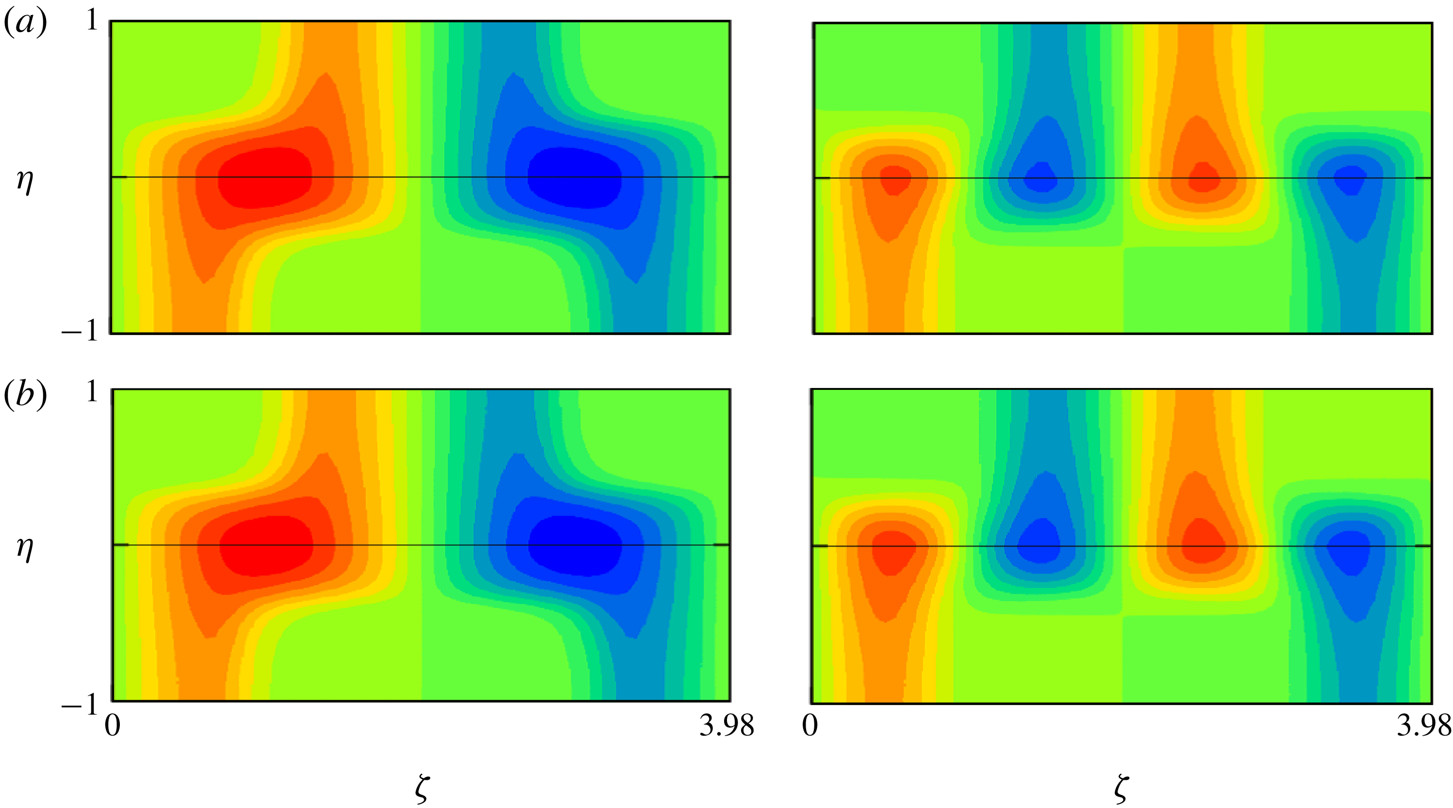
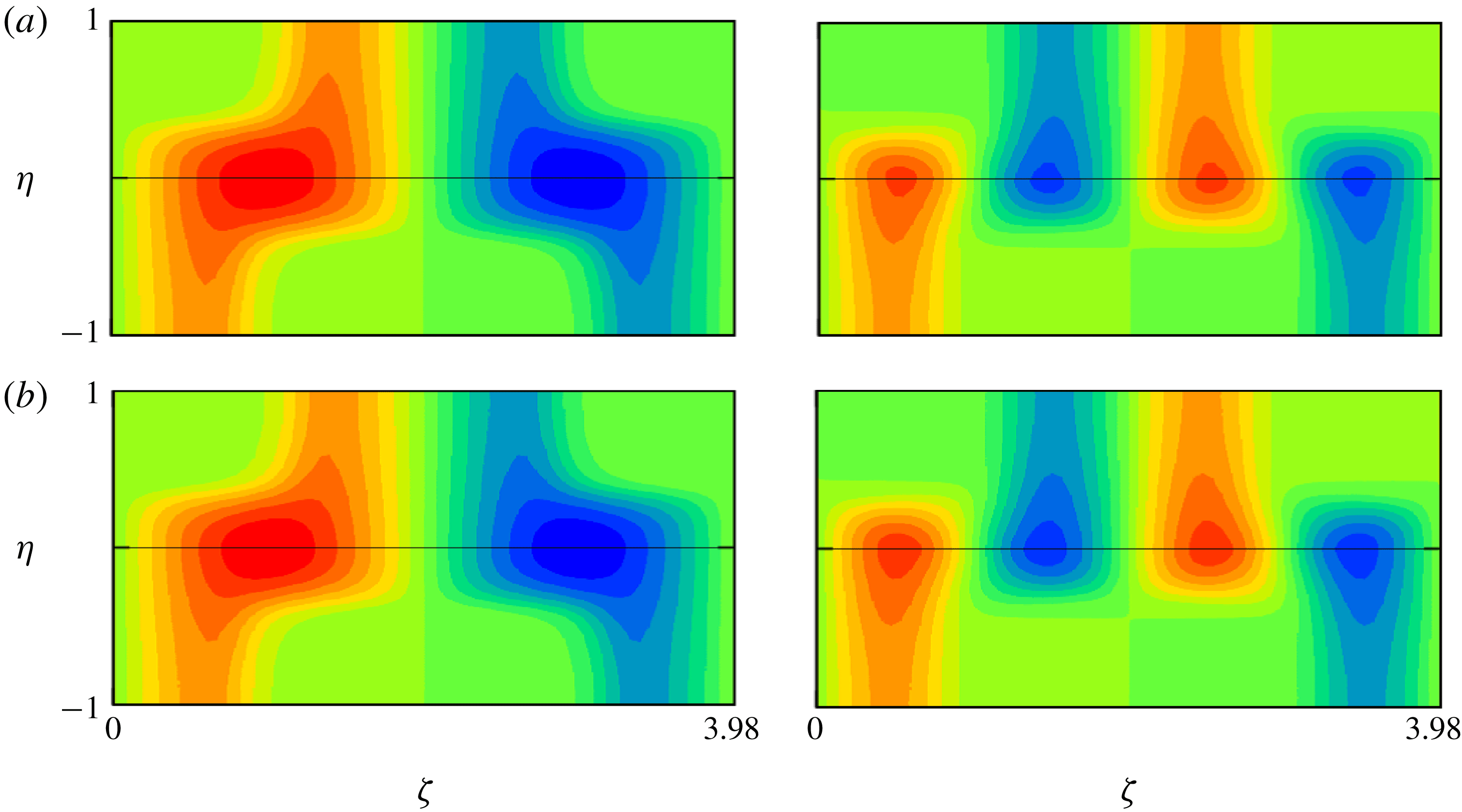
The pressure eigensolution on the right-hand branch of the full neutral curve in figure 1, for
 $R=10\,000$
. Panels (a) and (b) are the real part (
 $C_{max}=1$
) and the imaginary part (
 $C_{max}=0.2$
), respectively. The black solid curve is the critical curve.

In theory, we can first compute the canonical basis functions such as
 $\widetilde{f}(n,\unicode[STIX]{x1D701};\text{e}^{\text{i}m\unicode[STIX]{x1D6FD}\unicode[STIX]{x1D701}})$
by numerically solving (3.15), and then seek the special value of
 $\unicode[STIX]{x1D6FC}$
that makes the matrix
 $\unicode[STIX]{x1D648}$
singular; alternatively, we can treat
 $\unicode[STIX]{x1D6FC}^{2}$
as an eigenvalue, as we shall see shortly. However, it turns out that the canonical basis solutions typically take very large values near the walls at
 $\unicode[STIX]{x1D702}=\pm 1$
, and hence using them in the entire domain leads to numerical inaccuracy. Therefore, it is more sensible to use the canonical basis functions only for
 $|\unicode[STIX]{x1D702}|<\unicode[STIX]{x1D702}_{0}$
, where we choose
 $\unicode[STIX]{x1D702}_{0}=0.2$
for the model profile. As long as
 $\unicode[STIX]{x1D702}_{0}>0$
is chosen to be not too large, the canonical basis functions behave well and any fine tuning is unnecessary here.
For
 $|\unicode[STIX]{x1D702}|>\unicode[STIX]{x1D702}_{0}$
, the usual Chebyshev collocation method can be employed to solve (3.13). In this outer zone, the pressure
 $p$
is determined by the spectral coefficients
 $\unicode[STIX]{x1D711}_{m,l}$
multiplied by the
 $l$
th Chebyshev polynomials and the
 $m$
th Fourier harmonics. At
 $\unicode[STIX]{x1D702}=\pm \unicode[STIX]{x1D702}_{0}$
, we require that
 $p$
and
 $p_{\unicode[STIX]{x1D702}}$
are continuous. The unknowns associated with those conditions are, of course,
 $a_{m}$
and
 $b_{m}$
, which fixes
 $p$
within the inner zone
 $|\unicode[STIX]{x1D702}|<\unicode[STIX]{x1D702}_{0}$
. Evaluating (3.13) at the suitable collocation points, together with the boundary conditions on the walls, and the continuity of
 $p$
and
 $p_{\unicode[STIX]{x1D702}}$
, we have an eigenvalue problem
 $$\begin{eqnarray}\displaystyle \unicode[STIX]{x1D648}_{1}\left[\begin{array}{@{}c@{}}a_{m}\\ b_{m}\\ \unicode[STIX]{x1D711}_{m,l}\end{array}\right]=\unicode[STIX]{x1D6FC}^{2}\unicode[STIX]{x1D648}_{2}\left[\begin{array}{@{}c@{}}a_{m}\\ b_{m}\\ \unicode[STIX]{x1D711}_{m,l}\end{array}\right], & & \displaystyle\end{eqnarray}$$
which can, for example, be solved by the LAPACK routine. (Note that (3.13), (3.15) and (3.17) can be separated into the part proportional to
 $\unicode[STIX]{x1D6FC}^{2}$
and the rest.) Here, as usual, the unphysical eigenvalues associated with the boundary conditions must be removed (see Boyd Reference Boyd2001). For more general flows, we must assume the value of
 $c$
to compute the flow-fitted coordinates. If a positive purely real value cannot be found in the eigenvalues
 $\unicode[STIX]{x1D6FC}^{2}$
, the computation must be repeated varying
 $c$
.

For the steady mode of the model flow (3.12), this iteration is not necessary, and the numerical result indeed predicts the critical value
 $\unicode[STIX]{x1D6FC}=1.16$
, at which the right-hand branch of the full neutral curve tends to
 $R\rightarrow \infty$
(figure 3). The comparison of the pressure eigenmodes shown in figure 5 also confirms that the solution of the limiting inviscid problem indeed provides excellent predictions for the full linear Navier–Stokes result. In figure 3 we also note that for the left-hand branch viscosity is not negligible everywhere, because the small critical wavenumber of
 $O(R^{-1})$
ensures the viscous–convective balance.
4 Conclusion
The inviscid limit of the linear instability occurring in a unidirectional shear flow sheared in two transverse directions has been studied. The sufficient condition for the existence of a neutral mode is given in § 3.1. The new numerical method developed in § 3.2 led us to the first accurate numerical computation of singular neutral modes.
The new numerical method is tested against the simple model flow (3.12) in § 3. The model flow has a similar shape to the streak field of the steady nonlinear plane Couette solution used in figure 1. Thus not surprisingly the same methodology can be used to produce the red circle in figure 1. Again, the result is consistent with the large-Reynolds-number computation based on the linearised Navier–Stokes equations. In the vortex–wave interaction framework, this neutral mode is exactly the one maintaining the steady roll streak. Therefore, the accurate computation of it is indispensable to completely remove the Reynolds-number (or the regularisation-parameter) dependence from the asymptotically reduced system. The delicate singular structure is also important in estimating the stability of the solution, as shown by Deguchi & Hall (Reference Deguchi and Hall2016). The importance of the singular neutral solution of (1.2) is not limited to purely hydrodynamic problems; see the vortex–wave interaction theory formulated for weakly stratified flows by Deguchi (Reference Deguchi2017) and Olvera & Kerswell (Reference Olvera and Kerswell2017). Moreover, it was recently shown by Deguchi (Reference Deguchi2019) that it appears as a part of the self-sustained magnetohydrodynamic dynamo process at large Reynolds numbers.
The proposed algorithm can be utilised for quite general background flows as long as the critical layers do not intersect each other (i.e. the shear does not vanish along the critical level). An interesting case is the generalised Couette flow between wavy walls. In this case, since
 $\unicode[STIX]{x0394}U=0$
is satisfied,
 $\unicode[STIX]{x1D702}$
and
 $\unicode[STIX]{x1D701}$
are harmonic functions and can be found analytically. The method can also be used for non-circular pipe flows, or more complicated forced flows with many critical layers. In the latter case, complication of the numerical code may be unavoidable, but a general code could be developed by combining the local basis around the critical layer constructed here and the spectral/hp method (Karniadakis & Sherwin Reference Karniadakis and Sherwin2005).
It should also be remarked that the new method is more numerically economical than the large-Reynolds-number computation of the linearised Navier–Stokes equations, where the three velocity components and the pressure (or two potentials) must be solved. Near the critical level, the amplitude of the perturbation velocity behaves like
 $n^{-1}$
, and this singular behaviour must be reconciled within the critical layer of thickness
 $R^{-1/3}$
. The bottleneck of the stability analysis is the algebraic linear eigenvalue problem part because the high resolution required to resolve the asymptotically sharp flow structure makes the stability matrix huge. On the other hand, here we solve a single equation for the pressure, and no sharp structure appears when it is converted to the Frobenius form.
Acknowledgements
This work is supported by Australian Research Council Discovery Early Career Researcher Award DE170100171. The author acknowledges the anonymous referees who carefully checked the equations and grammatical errors, and gave many helpful comments that significantly improved the clarity of this paper.
Appendix A. Critical layer analysis
Here we use the body-fitted coordinates. The flow inside the critical layer can be analysed by using the stretched variable
 $N=n/\unicode[STIX]{x1D6FF}$
with the critical layer thickness
 $\unicode[STIX]{x1D6FF}=R^{-1/3}$
. As usual, here we omit the analysis of terms involving
 $\ln \unicode[STIX]{x1D6FF}$
(the terms of logarithmic order match automatically and hence do not need to be considered separately). The appropriate inner expansions are
 $$\begin{eqnarray}\displaystyle \left.\begin{array}{@{}c@{}}\displaystyle p=P_{0}(s)+\unicode[STIX]{x1D6FF}^{2}P_{2}(N,s)+\unicode[STIX]{x1D6FF}^{3}P_{3}(N,s)+\cdots \,,\\ \displaystyle u=\unicode[STIX]{x1D6FF}^{-1}U_{0}(N,s)+U_{1}(N,s)+\cdots \,,\\ \displaystyle (v,w)\boldsymbol{\cdot }\boldsymbol{e}_{n}=V_{0}(N,s)+\unicode[STIX]{x1D6FF}V_{1}(N,s)+\cdots \,,\\ \displaystyle (v,w)\boldsymbol{\cdot }\boldsymbol{e}_{s}=\unicode[STIX]{x1D6FF}^{-1}W_{0}(N,s)+W_{1}(N,s)+\cdots \,.\end{array}\right\} & & \displaystyle\end{eqnarray}$$
In order to match the critical layer solution to the outer solution,
 $P_{0},~N^{-2}P_{2},~N^{-3}P_{3}$
,
 $NU_{0}$
,
 $U_{1},~V_{0},~N^{-1}V_{1},~NW_{0}$
and
 $W_{1}$
must tend to
 $O(N^{0})$
quantities as
 $|N|\rightarrow \infty$
. From the cross-streamwise components of (2.1), we can deduce the critical layer equations
 $$\begin{eqnarray}\displaystyle \left.\begin{array}{@{}c@{}}\displaystyle {\mathcal{S}}V_{0}=-P_{2N},\quad {\mathcal{S}}V_{1}+\text{i}\unicode[STIX]{x1D6FC}\unicode[STIX]{x1D706}_{2}N^{2}V_{0}=-P_{3N}+\unicode[STIX]{x1D712}V_{0N},\\ \displaystyle {\mathcal{S}}W_{0}=-P_{0}^{\prime },\quad {\mathcal{S}}W_{1}+\text{i}\unicode[STIX]{x1D6FC}\unicode[STIX]{x1D706}_{2}N^{2}W_{0}=\unicode[STIX]{x1D712}W_{0N},\end{array}\right\} & & \displaystyle\end{eqnarray}$$
where
 ${\mathcal{S}}=\{\text{i}\unicode[STIX]{x1D6FC}\unicode[STIX]{x1D706}_{1}N-\unicode[STIX]{x2202}_{N}^{2}\}$
. The far-field behaviour of the functions
 $V_{0},~W_{0}$
and
 $W_{1}$
must be consistent with those of
 $P_{0}$
and
 $P_{2}$
where there should be no jump according to the Frobenius expansion (3.4). Hence
 $[V_{0},NW_{0},W_{1}](N,s)$
tend to
 $[\widehat{V}_{0},\widehat{W}_{0},\widehat{W}_{1}](s)$
as
 $|N|\rightarrow \infty$
. The jump may appear in
 $V_{1}$
, which is linked to
 $P_{3}$
. Using the streamwise component of the momentum equation and the continuity equation, the higher-order critical layer equations can be combined to yield
 $$\begin{eqnarray}\displaystyle \hspace{-20.00003pt}{\mathcal{S}}V_{1NN}=\text{i}\unicode[STIX]{x1D6FC}\{2\unicode[STIX]{x1D706}_{2}V_{0}+2\unicode[STIX]{x1D706}_{1}^{\prime }(NW_{1})_{N}+(2\unicode[STIX]{x1D706}_{2}^{\prime }-\unicode[STIX]{x1D712}\unicode[STIX]{x1D706}_{1}^{\prime })(N^{2}W_{0})_{N}+\unicode[STIX]{x1D712}\unicode[STIX]{x1D706}_{1}(N^{2}W_{0s})_{N}\}+H, & & \displaystyle\end{eqnarray}$$
where
 $H(N,s)\rightarrow 0$
as
 $|N|\rightarrow \infty$
. Therefore, the solution must have the form
 $$\begin{eqnarray}\left.\begin{array}{@{}c@{}}\displaystyle V_{1}=\frac{\text{i}\unicode[STIX]{x1D6FC}\{2\unicode[STIX]{x1D706}_{2}\widehat{V}_{0}+2\unicode[STIX]{x1D706}_{1}^{\prime }\widehat{W}_{1}+(2\unicode[STIX]{x1D706}_{2}^{\prime }-\unicode[STIX]{x1D712}\unicode[STIX]{x1D706}_{1}^{\prime })\widehat{W}_{0}+\unicode[STIX]{x1D712}\unicode[STIX]{x1D706}_{1}\widehat{W}_{0}^{\prime }\}}{(\unicode[STIX]{x1D6FC}|\unicode[STIX]{x1D706}_{1}|)^{4/3}}F(\unicode[STIX]{x1D709})+h(N,s),\\ \displaystyle \unicode[STIX]{x1D709}=(\unicode[STIX]{x1D6FC}|\unicode[STIX]{x1D706}_{1}|)^{1/3}N,\end{array}\right\}\end{eqnarray}$$
where
 $h(N,s)\rightarrow 0$
as
 $|N|\rightarrow \infty$
and
 $F(\unicode[STIX]{x1D709})$
satisfies
 $\{\text{i}\,\text{sgn}(\unicode[STIX]{x1D706}_{1})\unicode[STIX]{x1D709}-\unicode[STIX]{x2202}_{\unicode[STIX]{x1D709}}^{2}\}F_{\unicode[STIX]{x1D709}\unicode[STIX]{x1D709}}=1$
. The asymptotic behaviour
 $-\text{i}F_{\unicode[STIX]{x1D709}}\rightarrow {\mathcal{L}}(\unicode[STIX]{x1D709})+\text{(regular part)}$
with
 $\unicode[STIX]{x1D703}=-\unicode[STIX]{x03C0}\,\text{sgn}(\unicode[STIX]{x1D706}_{1})$
as
 $|\unicode[STIX]{x1D709}|\rightarrow \infty$
is well known in the asymptotic study of shear flow instability (see Lin Reference Lin1955; Haberman Reference Haberman1972; Deguchi & Walton Reference Deguchi and Walton2018; and references therein).
Appendix B. Property of the flow-fitted coordinates
The differentiation of a function
 $\unicode[STIX]{x1D719}$
in the
 $(\unicode[STIX]{x1D702},\unicode[STIX]{x1D701})$
coordinates can be found by the chain rule as
 $$\begin{eqnarray}\displaystyle \left[\begin{array}{@{}c@{}}\unicode[STIX]{x1D719}_{\unicode[STIX]{x1D702}}\\ \unicode[STIX]{x1D719}_{\unicode[STIX]{x1D701}}\end{array}\right]=\left[\begin{array}{@{}cc@{}}y_{\unicode[STIX]{x1D702}} & z_{\unicode[STIX]{x1D702}}\\ y_{\unicode[STIX]{x1D701}} & z_{\unicode[STIX]{x1D701}}\end{array}\right]\left[\begin{array}{@{}c@{}}\unicode[STIX]{x1D719}_{y}\\ \unicode[STIX]{x1D719}_{z}\end{array}\right]. & & \displaystyle\end{eqnarray}$$
If the determinant
 $$\begin{eqnarray}\displaystyle J=y_{\unicode[STIX]{x1D702}}z_{\unicode[STIX]{x1D701}}-y_{\unicode[STIX]{x1D701}}z_{\unicode[STIX]{x1D702}}, & & \displaystyle\end{eqnarray}$$
is non-vanishing, the inverse transformation can be obtained as
 $$\begin{eqnarray}\displaystyle \left[\begin{array}{@{}c@{}}\unicode[STIX]{x1D719}_{y}\\ \unicode[STIX]{x1D719}_{z}\end{array}\right]=\frac{1}{J}\left[\begin{array}{@{}cc@{}}z_{\unicode[STIX]{x1D701}} & -z_{\unicode[STIX]{x1D702}}\\ -y_{\unicode[STIX]{x1D701}} & y_{\unicode[STIX]{x1D702}}\end{array}\right]\left[\begin{array}{@{}c@{}}\unicode[STIX]{x1D719}_{\unicode[STIX]{x1D702}}\\ \unicode[STIX]{x1D719}_{\unicode[STIX]{x1D701}}\end{array}\right]. & & \displaystyle\end{eqnarray}$$
Replacing
 $\unicode[STIX]{x1D719}$
by
 $\unicode[STIX]{x1D702}$
or
 $\unicode[STIX]{x1D701}$
in the above equations,
 $$\begin{eqnarray}\displaystyle \unicode[STIX]{x1D702}_{y}=\frac{z_{\unicode[STIX]{x1D701}}}{J},\quad \unicode[STIX]{x1D701}_{y}=-\frac{z_{\unicode[STIX]{x1D702}}}{J},\quad \unicode[STIX]{x1D702}_{z}=-\frac{y_{\unicode[STIX]{x1D701}}}{J},\quad \unicode[STIX]{x1D701}_{z}=\frac{y_{\unicode[STIX]{x1D702}}}{J}. & & \displaystyle\end{eqnarray}$$
Given the first derivatives (B 3), we can show that the two-dimensional Laplace operator becomes
 $$\begin{eqnarray}\displaystyle \unicode[STIX]{x0394}\unicode[STIX]{x1D719} & = & \displaystyle \frac{1}{J}\left\{\left(\frac{y_{\unicode[STIX]{x1D701}}^{2}+z_{\unicode[STIX]{x1D701}}^{2}}{J}\unicode[STIX]{x1D719}_{\unicode[STIX]{x1D702}}\right)_{\!\unicode[STIX]{x1D702}}+\left(\frac{y_{\unicode[STIX]{x1D702}}^{2}+z_{\unicode[STIX]{x1D702}}^{2}}{J}\unicode[STIX]{x1D719}_{\unicode[STIX]{x1D701}}\right)_{\!\unicode[STIX]{x1D701}}\right\}\nonumber\\ \displaystyle & = & \displaystyle (\unicode[STIX]{x0394}\unicode[STIX]{x1D702})\unicode[STIX]{x1D719}_{\unicode[STIX]{x1D702}}+(\unicode[STIX]{x0394}\unicode[STIX]{x1D701})\unicode[STIX]{x1D719}_{\unicode[STIX]{x1D701}}+(\unicode[STIX]{x1D702}_{y}^{2}+\unicode[STIX]{x1D702}_{z}^{2})\unicode[STIX]{x1D719}_{\unicode[STIX]{x1D702}\unicode[STIX]{x1D702}}+(\unicode[STIX]{x1D701}_{y}^{2}+\unicode[STIX]{x1D701}_{z}^{2})\unicode[STIX]{x1D719}_{\unicode[STIX]{x1D701}\unicode[STIX]{x1D701}}.\end{eqnarray}$$
Here in order to calculate the second line we have used
 $$\begin{eqnarray}\displaystyle \left.\begin{array}{@{}c@{}}\displaystyle \unicode[STIX]{x1D701}_{y}^{2}+\unicode[STIX]{x1D701}_{z}^{2}=\frac{y_{\unicode[STIX]{x1D702}}^{2}+z_{\unicode[STIX]{x1D702}}^{2}}{J^{2}},\quad \unicode[STIX]{x1D702}_{y}^{2}+\unicode[STIX]{x1D702}_{z}^{2}=\frac{y_{\unicode[STIX]{x1D701}}^{2}+z_{\unicode[STIX]{x1D701}}^{2}}{J^{2}},\\ \displaystyle \unicode[STIX]{x0394}\unicode[STIX]{x1D702}=\frac{1}{J}\left(\frac{y_{\unicode[STIX]{x1D701}}^{2}+z_{\unicode[STIX]{x1D701}}^{2}}{J}\right)_{\!\unicode[STIX]{x1D702}},\quad \unicode[STIX]{x0394}\unicode[STIX]{x1D701}=\frac{1}{J}\left(\frac{y_{\unicode[STIX]{x1D702}}^{2}+z_{\unicode[STIX]{x1D702}}^{2}}{J}\right)_{\!\unicode[STIX]{x1D701}},\end{array}\right\} & & \displaystyle\end{eqnarray}$$
found from (B 4) and the first line of (B 5). There is another set of useful formulae obtained by the chain rule:
 $$\begin{eqnarray}\frac{\unicode[STIX]{x2202}y}{\unicode[STIX]{x2202}y}=\unicode[STIX]{x1D702}_{y}y_{\unicode[STIX]{x1D702}}+\unicode[STIX]{x1D701}_{y}y_{\unicode[STIX]{x1D701}}=1,\quad \frac{\unicode[STIX]{x2202}y}{\unicode[STIX]{x2202}z}=\unicode[STIX]{x1D702}_{z}y_{\unicode[STIX]{x1D702}}+\unicode[STIX]{x1D701}_{z}y_{\unicode[STIX]{x1D701}}=0,\end{eqnarray}$$
 $$\begin{eqnarray}\frac{\unicode[STIX]{x2202}z}{\unicode[STIX]{x2202}y}=\unicode[STIX]{x1D702}_{y}z_{\unicode[STIX]{x1D702}}+\unicode[STIX]{x1D701}_{y}z_{\unicode[STIX]{x1D701}}=0,\quad \frac{\unicode[STIX]{x2202}z}{\unicode[STIX]{x2202}z}=\unicode[STIX]{x1D702}_{z}z_{\unicode[STIX]{x1D702}}+\unicode[STIX]{x1D701}_{z}z_{\unicode[STIX]{x1D701}}=1.\end{eqnarray}$$
Then (B 7) and (3.10) can be used to deduce (3.11) and
 $(y_{\unicode[STIX]{x1D701}},z_{\unicode[STIX]{x1D701}})=(\unicode[STIX]{x1D701}_{y},\unicode[STIX]{x1D701}_{z})/(\unicode[STIX]{x1D701}_{y}^{2}+\unicode[STIX]{x1D701}_{z}^{2})$
. Finally, those relationships and (B 4) allow us to further simplify the Laplace operator through
 $$\begin{eqnarray}\displaystyle \frac{\unicode[STIX]{x0394}\unicode[STIX]{x1D701}}{\unicode[STIX]{x1D702}_{y}^{2}+\unicode[STIX]{x1D702}_{z}^{2}}=\unicode[STIX]{x1D6EF}_{\unicode[STIX]{x1D701}},\quad \frac{\unicode[STIX]{x1D701}_{y}^{2}+\unicode[STIX]{x1D701}_{z}^{2}}{\unicode[STIX]{x1D702}_{y}^{2}+\unicode[STIX]{x1D702}_{z}^{2}}=2\unicode[STIX]{x1D6EF}, & & \displaystyle\end{eqnarray}$$
and hence the transformed Rayleigh equation (3.13) is obtained.