


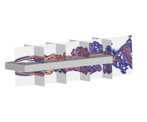



1. Introduction
The study of flow around bluff bodies with sharp corners holds great importance in engineering sciences, as it finds applications in various structures such as bridges, buildings and pylons (Tamura, Miyagi & Kitagishi Reference Tamura, Miyagi and Kitagishi1998). Among these bluff bodies, the rectangular cylinder serves as a simplified prototype. Despite its simple geometry, the flow around a rectangular cylinder exhibits intricate features, particularly the separation and reattachment of the unstable shear layer. As a result, it has garnered substantial attention in both fundamental research and industrial applications. Over the years, researchers have extensively investigated this flow phenomenon, recognizing its significance and relevance.
The flow behaviour around a rectangular cylinder is influenced by the aspect ratio, denoted as  $L/D$, where
 $L$ and
 $D$ represent the streamwise and cross-stream dimensions of the cylinder, respectively. When the aspect ratio is small (
 $1< L/D\le 3$), the shear layer separates from the leading edge (LE) and intermittently reattaches on the upper or lower side of the cylinder. However, for sufficiently large aspect ratios, the flow can permanently reattach and separate from the trailing edge (TE). Accurate classification of flow regimes based on aspect ratio also depends on the Reynolds number (
 $Re$), which is defined using the inflow velocity
 $U_0$ and
 $D$. When
 $Re$ exceeds 300, shedding of vortices from both the LE and TE occurs at the same frequency
 $f$, leading to an increase in the Strouhal number, given by
 $St(L)=f\kern0.7pt L/U_0$, in the two regimes. One regime is dominated by the LE vortex shedding, and
 $St(L)$ changes in a stepwise manner with increasing aspect ratio for
 $Re$ up to 2000 (Okajima Reference Okajima1982; Nakamura, Ohya & Tsuruta Reference Nakamura, Ohya and Tsuruta1991; Ozono et al. Reference Ozono, Ohya, Nakamura and Nakayama1992; Mills et al. Reference Mills, Sheridan, Hourigan and Welsh1995; Tan, Thompson & Hourigan Reference Tan, Thompson and Hourigan1998; Chiarini, Quadrio & Auteri Reference Chiarini, Quadrio and Auteri2022c; Zhang et al. Reference Zhang, Kareem, Xu and Jiang2023). The second regime, instead, is dominated by the TE vortex shedding, and
 $St(L)$ increases almost linearly with
 $L/D$ (Chiarini et al. Reference Chiarini, Quadrio and Auteri2022c). However, several experimental and numerical studies have shown that factors such as the blockage ratios of the open-water channel and computational domain, as well as flow disturbances from upstream of the cylinder, can affect this crucial characteristic of vortex shedding (Prasanth & Mittal Reference Prasanth and Mittal2008; Liu & Zhang Reference Liu and Zhang2015; Zhang & Liu Reference Zhang and Liu2015).
The impinging shear layer (ISL) instability and the impinging LE vortex (ILEV) instability were proposed by Nakamura & Nakashima (Reference Nakamura and Nakashima1986) and Naudascher & Rockwell (Reference Naudascher and Rockwell1994), respectively, to explain the frequency locking phenomenon and the stepwise dependence of  $St(L)$. Nakamura & Nakashima (Reference Nakamura and Nakashima1986) also speculated that the ISL instability is a one-sided phenomenon rather than relying on the interaction between shear layers from opposite sides. As a result of the ILEV instability, different shedding modes occur with distinct integer total numbers
 $n$ of LE vortices distributed on the upper and lower sides of the cylinder. With increasing
 $L/D$,
 $n$ also grows in a stepwise manner, leading to an approximate relationship of
 $St(L)\approx U_c {\cdot } n$, where
 $U_c$ is the mean convection velocity of LE vortices and is approximately 0.55 times the free stream velocity
 $U_0$ (Nakamura et al. Reference Nakamura, Ohya and Tsuruta1991; Mills, Sheridan & Hourigan Reference Mills, Sheridan and Hourigan2002; Tan, Thompson & Hourigan Reference Tan, Thompson and Hourigan2004; Chiarini et al. Reference Chiarini, Quadrio and Auteri2022c). Numerous studies have been conducted to investigate the stepwise phenomenon and explore the effects of TE vortices resulting from the ILEV instability (Hourigan et al. Reference Hourigan, Mills, Thompson, Sheridan, Dilin and Welsh1993; Hourigan, Thompson & Tan Reference Hourigan, Thompson and Tan2001; Mills et al. Reference Mills, Sheridan and Hourigan2002; Tan et al. Reference Tan, Thompson and Hourigan2004). Hourigan et al. (Reference Hourigan, Thompson and Tan2001) proposed that the flow instability relies on the interaction between LE vortices and TE vortices, with the shedding of TE vortices playing a crucial role in the self-sustained oscillation of the fluid. When a LE vortex passes over the TE, it generates a relatively weak pressure pulse that travels upstream and triggers the shedding of the LE vortex, completing the pressure feedback loop.
Recently, Chiarini et al. (Reference Chiarini, Quadrio and Auteri2022c) conducted a study on the variation of  $St(L)$ with the aspect ratio of rectangular cylinders at a Reynolds number of 400. The research encompassed numerous scenarios with different aspect ratios, including non-integer values. The authors asserted that the shedding of the TE vortices plays a central role in frequency locking based on their analysis of structural sensitivity. Two distinct flow configurations were identified, which exhibited a significant correlation with the interaction between the LE and TE vortices. When the LE vortex coincides in phase with the development of a new TE vortex on the same side, the overall frequency is determined by the shedding of the TE vortices. Conversely, when the LE vortex reaches the TE out of phase with the shedding of the TE vortex on the same side, it can induce the shedding of TE vortices on the opposite side. As a result, the shedding frequency is locked to the passing frequency of the LE vortices over the TE. In another study by Zhang et al. (Reference Zhang, Kareem, Xu and Jiang2023), three-dimensional unsteady flows around rectangular cylinders were investigated using large-eddy simulation (LES) at
 $Re=1000$. The aspect ratio of the cylinders ranged from 3 to 12. The researchers found that the phase difference between the LE and TE vortices is a critical factor contributing to the stepwise growth of
 $St(L)$ as
 $L/D$ increases. The self-sustained oscillation in the flow is sustained by two types of pressure feedback-loop mechanisms. For
 $L/D=4$ and
 $5$, the flow exhibits the ISL instability, and the separation region is covered by the pressure feedback loop. On the other hand, for
 $L/D=3$ and
 $L/D=6-12$, the flow is characterized by the ILEV instability along with the pressure feedback loop covering the entire rectangular cylinder.
Understanding the instability mechanism of flow around a rectangular cylinder is crucial for studying vortex dynamics and the generation of various structures. However, compared with the flow around circular cylinders (Jackson Reference Jackson1987; Monkewitz, Huerre & Chomaz Reference Monkewitz, Huerre and Chomaz1993; Giannetti & Luchini Reference Giannetti and Luchini2007; Marquet, Sipp & Jacquin Reference Marquet, Sipp and Jacquin2008) or square cylinders (Robichaux, Balachandar & Vanka Reference Robichaux, Balachandar and Vanka1999; Blackburn & Lopez Reference Blackburn and Lopez2003; Sheard, Fitzgerald & Ryan Reference Sheard, Fitzgerald and Ryan2009; Blackburn & Sheard Reference Blackburn and Sheard2010; Park & Yang Reference Park and Yang2016; Jiang, Cheng & An Reference Jiang, Cheng and An2018), the instability mechanism of this flow has received less attention. Chiarini, Quadrio & Auteri (Reference Chiarini, Quadrio and Auteri2021) investigated the primary instability of flow around a rectangular cylinder at low Reynolds numbers, considering the influence of the aspect ratio and the rounded LE and TE corners. The aspect ratio ranged from 0.25 to 30. They found that the primary instability results from a Hopf bifurcation, similar to the flow around a circular cylinder (Provansal, Mathis & Boyer Reference Provansal, Mathis and Boyer1987; Noack & Eckelmann Reference Noack and Eckelmann1994) or a square cylinder (Sohankar, Norberg & Davidson Reference Sohankar, Norberg and Davidson1999; Saha, Muralidhar & Biswas Reference Saha, Muralidhar and Biswas2000; Jiang & Cheng Reference Jiang and Cheng2018). The critical Reynolds number ( $Re_c$) for the primary instability increases from approximately 34.8 for
 $L/D=0.25$ to 140 for
 $L/D=30$. Direct numerical simulation (DNS) conducted by Hourigan et al. (Reference Hourigan, Thompson and Tan2001) focused on the three-dimensional flow around a rectangular cylinder at Reynolds numbers ranging from 350 to 400. They observed the formation of three-dimensional vortical structures on both sides of the cylinder and in the wake region. The hairpin-like vortical structures, arranged in a staggered manner, resemble ‘Pattern B’ structures identified by Sasaki & Kiya (Reference Sasaki and Kiya1991). Although the spanwise wake shedding modes are similar to those observed for a circular cylinder (referred to as ‘mode A’ and ‘mode B’) (Williamson Reference Williamson1988), the spanwise wavelengths are larger due to the thicker boundary layers near the TE, which lead to more diffused vortices. In a recent study by Chiarini, Quadrio & Auteri (Reference Chiarini, Quadrio and Auteri2022b), the three-dimensional instability of flow around a rectangular cylinder with an aspect ratio of 5 was investigated using Floquet analysis and DNS. A new quasisubharmonic (QS) unstable mode was discovered, which becomes unstable at approximately
 $Re=480$ with a spanwise wavelength
 $\lambda =2{\rm \pi} /k\approx 3$. This is different from the flow around cylinders with lower aspect ratios or smooth LEs. The structural sensitivity analysis revealed that the wavemaker region of the QS mode is located on the upper/lower side of the cylinder. Furthermore, the mutual inviscid interaction of vortices from the LE layer triggers the instability.
When the Reynolds number is sufficiently high, the flow exhibits significant turbulence. Cimarelli, Leonforte & Angeli (Reference Cimarelli, Leonforte and Angeli2018b) conducted the first investigation of this flow through DNS at  $L/D=5$ for
 $Re=3000$. Their findings revealed that the developed flow is predominantly characterized by quasistreamwise vortices and streamwise streaks induced by hairpin-like vortices. Conversely, reverse flow is characterized by spanwise vortices. They identified a self-sustaining mechanism in which large-scale pressure fluctuations alternate between promoting and suppressing the reverse flow, while small-scale motions trigger the formation of LE shear layers. Subsequently, Cimarelli, Leonforte & Angeli (Reference Cimarelli, Leonforte and Angeli2018a) explored the physical mechanisms driving the behaviour of separating and reattaching flows. The study by Cimarelli et al. (Reference Cimarelli, Leonforte, de Angelis, Crivellini and Angeli2019a) also unveiled negative turbulence production mechanisms in the LE shear layer. To gain further statistical insights into this flow, Chiarini & Quadrio (Reference Chiarini and Quadrio2021) conducted a comprehensive investigation of the single-point budget of Reynolds stresses at the same
 $Re$. The study focused on the most relevant production, redistribution and dissipation terms. Although the LE shear layer starts as laminar, its instability drains energy from the mean flow to feed downstream streamwise fluctuations. The other two components of turbulent kinetic energy (TKE) result from the redistribution of the streamwise TKE component driven by the pressure-strain term. In a study by Chiarini et al. (Reference Chiarini, Gatti, Cimarelli and Quadrio2022a), the contribution of structures with various scales to the sustaining mechanism was examined using anisotropic generalized Kolmogorov equations. The forward and reverse energy transfers occur simultaneously in this flow presented by the scale-space fluxes. The researchers identified two independent sources of velocity fluctuations: large Kelvin–Helmholtz (KH) rolls and small streamwise vortices. Near the TE, the turbulent structures are affected by the sudden disappearance of the wall, leading to a progressive vanishing of streamwise vortices and the transformation of spanwise structures into vertical fluctuations due to pressure-strain effects. In experimental research conducted by Moore, Letchford & Amitay (Reference Moore, Letchford and Amitay2019), separated shear layers from rectangular cylinders with aspect ratios of 5, 3 and 1 were investigated at Reynolds numbers ranging between
 $1.34\times 10^4$ and
 $1.18\times 10^5$. The study revealed that certain characteristics of the shear layer behaviour remained invariant as the Reynolds number changed, such as the time-averaged position of the shear layers. However, other characteristics were found to be dependent on the Reynolds number, including the spatial amplification of TKE.
Furthermore, the rectangular cylinder with an aspect ratio of  $L/D=5$ has emerged as the benchmark for studying the aerodynamics of the
 $5:1$ rectangular cylinder (BARC) (https://www.aniv-iawe.org/barc-docs). This benchmark was introduced during the 6th Colloquium on Bluff Body Aerodynamics and Applications, serving as a platform for scientists involved in bluff body aerodynamics research, with a particular focus on analysing turbulent separation flow around an elongated rectangular cylinder (Bruno, Salvetti & Ricciardelli Reference Bruno, Salvetti and Ricciardelli2014). Bruno et al. (Reference Bruno, Salvetti and Ricciardelli2014) conducted a comprehensive summary of experimental and numerical investigations related to the BARC. They found that lift generation is highly sensitive to test set-ups and modelling approaches, leading to notable discrepancies between experimental measurements and numerical predictions. Subsequently, Cimarelli et al. (Reference Cimarelli, Leonforte and Angeli2018a) performed well-converged statistical analyses that were unaffected by turbulence modelling, providing valuable insights into the quantification of numerical and modelling inaccuracies for relevant aerodynamic statistics. In addition, Cimarelli et al. (Reference Cimarelli, Leonforte, de Angelis, Crivellini and Angeli2019a) presented conceptual arguments for modelling turbulence production in the transitional shear layer, further expanding the understanding of this complex flow phenomenon. Moreover, Cimarelli et al. (Reference Cimarelli, Leonforte, de Angelis, Crivellini and Angeli2019b) utilized DNS data of the BARC flow to evaluate the combined influence of numerical resolution and subgrid turbulence closure on LES. Recently, Corsini et al. (Reference Corsini, Angeli, Stalio, Chibbaro and Cimarelli2022) presented a new and well resolved DNS around the BARC at
 $Re=3000$. Despite the use of different numerical methods and grids, their findings suggest that the primary differences can be attributed to the different grid spacings used. This serves as an initial exploration into studying the impact of spatial resolution in the DNS of flows around elongated rectangular cylinders with sharp corners.
As mentioned above, numerous studies have focused on investigating the flow behaviour around a rectangular cylinder. The influence of aspect ratio on the generation and evolution of vortex structures has primarily been examined at low  $Re$, while investigations at high
 $Re$ have generally concentrated on flows with an aspect ratio of
 $L/D=5$. However, there remains a dearth of research exploring the evolution of the boundary layer on the upper and lower sides of the rectangular cylinder at different aspect ratios, as well as the development of the wake. Consequently, the uniqueness of this study lies in its examination of vortex dynamics, encompassing the relationships between various flow processes and typical frequencies, the formation of hairpin vortices and hairpin vortex packets, and the interaction between the LE vortex and TE vortex. Additionally, the present work will propose mechanisms for the transition and relaminarization of the wall boundary layer to characterize its development. This investigation is conducted using DNS for a medium Reynolds number (
 $Re=1000$) and three different aspect ratios
 $L/D=5$,
 $10$ and
 $15$. To the best of the authors’ knowledge, such comprehensive research has not been previously reported. It is anticipated that the elucidation of the flow physics in this study will facilitate a deeper understanding of vortex dynamics, boundary layer transition, and reverse transition. The remainder of this paper is organized as follows: § 2 presents the physical model, numerical method and data analysis methods; the main findings are then discussed in § 3; finally, § 4 provides the conclusion.
2. Numerical methodology
2.1. Flow configuration and numerical method
Figure 1 shows a sketch of flow around a rectangular cylinder. The streamwise and vertical scales of the cylinder are  $L$ and
 $D$, respectively. The computational domain extends for
 $-10D\le x\le L+50D$ in the streamwise direction, for
 $-15.5D\le y\le 15.5D$ in vertical direction and
 $0\le z\le 2{\rm \pi} D$ in the spanwise direction. The fluid motion is described by the incompressible Navier–Stokes equations in dimensionless form, and are as follows:
 \begin{gather} \boldsymbol{\nabla}\boldsymbol{\cdot} \boldsymbol{u}=0, \end{gather}
 \begin{gather}\frac{\partial \boldsymbol{u}}{\partial t}+\boldsymbol{u}\boldsymbol{\cdot}\triangledown\boldsymbol{u}={-}\boldsymbol{\nabla} p+\frac{1}{Re}\nabla^{2}\boldsymbol{u}. \end{gather}
Here,  $\boldsymbol {u}\equiv (u,v,w)$ is the velocity vector,
 $t$ is the time and
 $p$ is the pressure. The Reynolds number
 $Re=U_0 D/\nu$ is defined based on the thickness of the rectangular cylinder
 $D$ and the inflow velocity
 $U_0$, where
 $\nu$ is the kinematic viscosity. In this study,
 $Re$ is fixed at 1000. Three aspect ratios (
 $L/D=5$,
 $10$,
 $15$) are considered.
Sketch of flow around a rectangular cylinder in an  $x$–
 $y$ plane. Here
 $L$ and
 $D$ are the streamwise and vertical dimensions of the rectangular cylinder, and
 $U_0$ is the inflow velocity.

A uniform flow velocity  $U_0$ is specified at the inlet boundary. The far-field condition (
 $\partial u/\partial y=0, v=0, \partial w/\partial y=0$) is imposed along the upper and lower surface of the domain. The high-order outflow boundary condition is imposed at the outlet (Dong, Karniadakis & Chryssostomidis Reference Dong, Karniadakis and Chryssostomidis2014). A no-slip boundary condition (
 $u=v=w=0$) is applied on the surface of the rectangular cylinder.
The Fourier spectral/ $hp$ element method (Bolis Reference Bolis2013) is used in the numerical simulations, which is embedded in the open-source code Nektar++ (Cantwell et al. Reference Cantwell2015; Moxey et al. Reference Moxey2020). A second-order implicit–explicit time integration scheme is chosen from the incompressible solver, and the time step is fixed at
 $0.001$. Applying this method, the problem is discretized spatially in the
 $x$–
 $y$ plane along with a Fourier expansion in the
 $z$ direction, revealing the three-dimensional features of the flow (Bolis Reference Bolis2013). In this study, the three-dimensional flow is resolved by performing a Fourier expansion in the spanwise direction, due to the assumption of being homogeneous in the spanwise direction (periodic conditions). In the spanwise direction,
 $N$ Fourier planes are used, and the spanwise resolution is
 $2N$. In the
 $x$–
 $y$ plane, the spatial resolution is determined by the distribution of
 $h$-type elements with
 $P$-order interpolation polynomials for the
 $p$-type expansion.
The simulations are first advanced for  $300D/U_0$ to allow for the flow to reach a truly statistically stationary state. When the flows reach the statistically steady state, the simulations accumulate statistics at each time step for further
 $200D/U_0$, while the sampling interval of the instantaneous three-dimensional flow fields is
 $0.25D/U_0$.
2.2. Validation and Mesh independence study
Figure 2 shows the macromesh in part of the domain for  $L/D=5$. In the present study, the polynomial order and the number of Fourier planes are set to
 $P=5$ and
 $N=96$ for all three cases, following the simulations at the same
 $Re$ in the studies of Li et al. (Reference Li, Wang, Qiu, Wu, Zhou, Fu and Liu2022a,Reference Li, Wang, Qiu, Wu, Zhou, Fu and Liub), in which the flow past a circular cylinder in proximity to a plane wall was investigated.
The partial domain with a macromesh for  $L/D=5$ in the
 $x$–
 $y$ plane. The inset is a close-up view of the mesh near the rectangular cylinder.

The Strouhal number  $St(L)$ based on the streamwise dimension of the rectangular cylinder is used to validate the present numerical model. The present results are shown in figure 3, compared with available experimental and numerical results carried out by Nakamura et al. (Reference Nakamura, Ohya and Tsuruta1991) and Zhang et al. (Reference Zhang, Kareem, Xu and Jiang2023), respectively. It can be found that the current
 $St(L)$ is in great agreement with the experimental results. The present results also match the LES results from Zhang et al. (Reference Zhang, Kareem, Xu and Jiang2023), although there is a very small deviation, which may be due to the difference in numerical methods.
The Strouhal number based on the streamwise dimension of the rectangular cylinder  $St(L)$ at different aspect ratios compared with the results from the literature.

For mesh independence check, the convergence of drag coefficient  $C_D$, the r.m.s. values of
 $C_D$ (
 $C_{D,rms}$) and r.m.s. values of lift coefficient
 $C_L$ (
 $C_{L,rms}$) are evaluated. The drag and lift coefficients are defined as
 \begin{equation} C_D=\frac{F_x}{0.5\rho D U^{2}_0},\quad C_L=\frac{F_y}{0.5\rho D U^{2}_0}, \end{equation}
where  $F_x$ and
 $F_y$ are the spanwise-averaged total forces acting on the rectangular cylinder in the streamwise and vertical directions, respectively. Here
 $\overline {C_D}$,
 $C_{D,rms}$ and
 $C_{L,rms}$ are shown in table 1 for different orders of polynomial interpolation
 $P$. Here, only the typical case at
 $L/D=5$ is displayed, as the other two aspect ratio cases are similar to it. Four meshes are generated along with
 $P$ varying from
 $4$ to
 $7$. It can be found that
 $\overline {C_D}$,
 $C_{D,rms}$ and
 $C_{L,rms}$ show good convergence as
 $P$ increases, when the time step is fixed at
 $0.001$ referring to the studies of Li et al. (Reference Li, Wang, Qiu, Wu, Zhou, Fu and Liu2022a,Reference Li, Wang, Qiu, Wu, Zhou, Fu and Liub). Therefore, it indicates that
 $P=5$ and
 $N=96$ are sufficient for current simulations.
Time-averaged drag coefficient  $\bar {C}_D$, the root-mean-square (r.m.s.) values of
 $C_D$, and the r.m.s. values of lift coefficient
 ${C_L}$ with different orders of polynomial interpolation
 $P$ at
 $Re=1000$ for
 $L/D=5$. Here
 $N_v$ is the number of elements,
 $N_d$ is approximate degree of freedom and
 $N$ is the number of Fourier planes.

2.3. Data analysis methods
2.3.1. Mode analyses
Dynamic mode decomposition (DMD) (Schmid Reference Schmid2010) and Fourier mode decomposition (FMD) (Basley et al. Reference Basley, Pastur, Lusseyran, Faure and Delprat2011; Ma et al. Reference Ma, Feng, Pan, Gao and Wang2015; Zhang & Zhou Reference Zhang and Zhou2024) are significant mode analysis tools, and were widely used in the previous studies (He, Wang & Pan Reference He, Wang and Pan2013; Wang et al. Reference Wang, Feng, Wang and Li2018; Wang & Wang Reference Wang and Wang2021a,Reference Wang and Wangb; Li et al. Reference Li, Wang, Qiu, Wu, Zhou, Fu and Liu2022a).
The DMD can extract a set of modes from the original unsteady dynamic flow. Each mode is associated with the spatial structures in the flow field, which is dominant at a certain frequency. Therefore, DMD can be applied to extract the dominant modes with characteristic frequencies. The snapshots of the flow fields can be decomposed as
 \begin{gather} \varPhi(\boldsymbol{x},t)=\boldsymbol{U}(\boldsymbol{x})+\sum_{k=1}^{r}b_k\phi_k(\boldsymbol{x})\, {\rm e}^{\omega_k t}, \end{gather}
 \begin{gather}\omega_k=\log(\mu_k)/{\Delta t}, \end{gather}
here,  $U$,
 $\varPhi$,
 $\phi _k$,
 $b_k$,
 $\mu _k$ are the mean field, reconstructed field,
 $k$th DMD mode, the magnitude of the
 $k$th DMD mode and the eigenvalue of the
 $k$th mode, respectively. In present study, DMD analysis is based on the three-dimensional flow fields, and each sample consists of the three velocity components
 $u$,
 $v$ and
 $w$ to extract the typical flow structures.
Different typical frequencies are generated due to the shedding of the LE vortex or TE vortex. The reconstructions of the fluctuating velocity with different frequencies could help to investigate the vortex dynamics of the shear layer. The FMD is conducted by applying single-point discrete Fourier transformation to fluctuating velocity sequence. A Fourier-transform matrix  $\boldsymbol {v}_k$ is obtained as follows:
 \begin{equation} \boldsymbol{v}_k=\frac{1}{M}\sum_{m=0}^{M-1}\boldsymbol{F}_m \,{\rm e}^{-{\rm i}(2{\rm \pi} k/M)m}, \end{equation}
where  $M$ and
 $\boldsymbol {F}_m$ are the total number of the samples and the matrix of fluctuating velocity sequences, respectively. The fluctuating velocity with different frequency bands
 $\boldsymbol {F}_m^{band}$ can be reconstructed by using inverse Fourier transformation to
 $\boldsymbol {v}_k$:
 \begin{equation} \boldsymbol{F}_m^{band}=\sum_{band}\boldsymbol{v}_k \,{\rm e}^{{\rm i}(2{\rm \pi} k/M)m}. \end{equation}
2.3.2. Finite-time Lyapunov exponents method
The finite-time Lyapunov exponents (FTLEs) method can track Lagrangian coherent structures (LCSs) successfully (Haller & Yuan Reference Haller and Yuan2000; Haller Reference Haller2001; Shadden, Dabiri & Marsden Reference Shadden, Dabiri and Marsden2006; Green, Rowley & Haller Reference Green, Rowley and Haller2007; Shadden, Astorino & Gerbeau Reference Shadden, Astorino and Gerbeau2010), especially in complex flows (He et al. Reference He, Pan, Feng, Gao and Wang2016; Wang et al. Reference Wang, Feng, Wang and Li2018; Wang & Wang Reference Wang and Wang2021a,Reference Wang and Wangb; Cheng et al. Reference Cheng, Jiang, Chong, Zhou, Liu and Lu2022). The flow map is denoted by  $\varPhi _{t_0}^{t_0+t_1}:\boldsymbol {x}(t_0)\longrightarrow \boldsymbol {x}(t_0+t_1)$, which maps fluid particles from the initial location
 $\boldsymbol {x}(t_0)$ at time
 $t_0$ to the location
 $\boldsymbol {x}(t_0+t_1)$ at
 $t_0+t_1$. The FTLE at
 $t_0$ can be calculated as follows:
 \begin{equation} \sigma (\boldsymbol{x},t_0,t_1)=\frac{1}{| 2t_1 | }\ln\left ( \lambda_{max}\left \{ \left [\frac{\partial \boldsymbol{x}(t_0+t_1) }{\partial \boldsymbol{x}(t_0)} \right ]^{\rm T} \left [ \frac{\partial \boldsymbol{x}(t_0+t_1)}{\partial \boldsymbol{x}(t_0)} \right ] \right \} \right ), \end{equation}
here,  $\sigma (\boldsymbol {x},t_0,t_1)$ is the exponential growth rate of nearby trajectories over a finite time interval
 $t_1$, and
 $\lambda _{max}$ denotes the largest singular value of the deformation gradient matrix. In the current work,
 $t_1<0$ is used to conduct backward computations to obtain the ridges of LCSs
 $\sigma (\boldsymbol {x},t_0,t_1)$.
3. Results and discussion
3.1. Vortex dynamics
In this section, the effects of aspect ratio on the vortex dynamics around a rectangular cylinder are examined. The visualization of instantaneous vortical structures are presented first, including the evolutions of different vortex structures. Then the typical characteristics of mean flow statistics are discussed, contributing to an overview of the vortex generation and evolution. Furthermore, the vortex dynamics associated with several prominent frequencies are discussed.
3.1.1. Instantaneous vortical structures and mean flow statistics
Figure 4 illustrates the instantaneous three-dimensional vortical structures for the three different aspect ratios, identified through the  $Q$ criterion with
 $Q=0.1$. Since the flows exhibit symmetry, the evolution processes of various vortex structures on the upper side of the cylinder will be described only. For
 $L/D=5$ in figure 4(a), the onset of KH instability is observed in the LE shear layer, resulting in the formation of spanwise KH vortices. The subsequent secondary instability of the KH vortex indicates its limited persistence over a short range. This secondary destabilized KH vortex then transforms into the LE vortices, as also noted in the study by Zhang et al. (Reference Zhang, Kareem, Xu and Jiang2023). However, the present DNS results provide clearer identification of hairpin vortices compared with previous studies. These hairpin vortices arise from the LE vortices due to the background mean shear. The intense shear effects cause regions of high momentum to form the head of the hairpin vortices, while regions of low momentum develop into their legs. This generation process of hairpin vortices is akin to that observed in the interaction between the wake of a circular cylinder and a wall boundary at a very small gap ratio (Li et al. Reference Li, Wang, Qiu, Wu, Zhou, Fu and Liu2022a). Although these two flow configurations are different, the hairpin vortices in both flows are evolved from KH vortices. Furthermore, the LE vortices composed of multiple hairpin vortices appear more irregular than those observed at lower Reynolds numbers in the studies of Hourigan et al. (Reference Hourigan, Thompson and Tan2001) and Chiarini et al. (Reference Chiarini, Quadrio and Auteri2022b). It should be noted that the scale of hairpin vortices appears larger than the results reported by Cimarelli et al. (Reference Cimarelli, Leonforte and Angeli2018b), Chiarini & Quadrio (Reference Chiarini and Quadrio2021) and Chiarini et al. (Reference Chiarini, Gatti, Cimarelli and Quadrio2022a), which can be attributed to the higher Reynolds numbers employed in their investigations.
Instantaneous three-dimensional vortical structures visualized by isosurfaces of  $Q=0.1$, coloured with the instantaneous streamwise velocity
 $u/U_0$: (a)
 $L/D=5$; (b)
 $L/D=10$; (c)
 $L/D=15$.

The mean shear, denoted as  $\tau = ({1}/{Re}) ({\partial U}/{\partial y})$, is illustrated in figure 5. The figure clearly demonstrates the presence of strong shear in the LE shear layer and the forward wall boundary layer after the reattachment. Furthermore, it can be observed that as the aspect ratio increases, the duration of the mean shear becomes longer, resulting in a greater amount of shear experienced by the flow. Consequently, the intensified mean shear in cases with larger aspect ratios significantly impacts the evolution of hairpin vortices.
Mean shear  $\tau /U_0^2$: (a)
 $L/D=5$; (b)
 $L/D=10$; (c)
 $L/D=15$.

The vortical structures associated with larger aspect ratios have received limited attention in previous researches. Figure 4(b,c) demonstrate that the generation and three-dimensional instability processes of the KH vortices at  $L/D=10$ and
 $15$ are similar to those observed at
 $L/D=5$. Nevertheless, the formation of KH vortices is observed to take place at larger distances from the LE as the aspect ratio increases. The evolution of KH rolls into hairpin vortices along the shear layer is less abrupt as the aspect ratio increases, although the mean shear increases. The increased streamwise dimension of the rectangular cylinder allows the hairpin vortices to travel farther downstream along the wall at larger aspect ratio. As they progress downstream, the hairpin vortices experience stretching due to the enhanced mean shear. The high-momentum heads of the hairpin vortices tend to be lifted up, leading to the formation of hairpin vortex packets for both aspect ratios (
 $L/D=10$ and
 $15$). Furthermore, despite a portion of the packet being convected downstream of the TE, the hairpin vortex packet retains its shape due to memory effects.
For all three aspect ratios, the TE vortex is generated and subsequently sheds into the wake. However, it is evident that the wake for  $L/D=5$ exhibits larger-scale oscillations in the vertical direction compared with the other two aspect ratios. At the current medium Reynolds number, the oscillation in the
 $L/D=5$ flow appears to be more apparent than what was observed in the studies conducted by Cimarelli et al. (Reference Cimarelli, Leonforte and Angeli2018b), Chiarini & Quadrio (Reference Chiarini and Quadrio2021) and Chiarini et al. (Reference Chiarini, Gatti, Cimarelli and Quadrio2022a) at a high Reynolds number (
 $Re=3000$). This can be observed not only in the instantaneous vortical structures, but also quantitatively reflected in
 $C_{L,rms}$. Specifically, at
 $L/D=5$, the present work reports a value of
 $C_{L,rms}=0.71$, as shown in table 1. This is larger than the value of
 $C_{L,rms}=0.29$ obtained under the same aspect ratio for
 $Re=3000$ (Chiarini & Quadrio Reference Chiarini and Quadrio2021). Furthermore, the wakes for all three aspect ratios exhibit a Kármán-like vortex street formation, which has rarely been paid close attention to in studies investigating high Reynolds number (Cimarelli et al. Reference Cimarelli, Leonforte and Angeli2018b; Chiarini & Quadrio Reference Chiarini and Quadrio2021; Chiarini et al. Reference Chiarini, Gatti, Cimarelli and Quadrio2022a).
Figure 6(a,c,e) present the time and spanwise-averaged streamwise velocity  $U/U_0$ for
 $L/D=5$,
 $10$ and
 $15$, respectively, in pseudocolour with the superimposition of streamlines. Due to the flow symmetry, the discussion of mean flow statistics focuses solely on the upper side of the cylinder as well. The observations reveal a consistent flow behaviour across all three aspect ratios. The flow separates at the LE and subsequently reattaches downstream on the upper side of the rectangular cylinder. This phenomenon gives rise to the formation of separation bubbles. The streamwise scales of these separation bubbles are found to be
 $4.42D$,
 $6.28D$,
 $7.12D$ for aspect ratios of
 $L/D=5$, 10, 15, respectively. Additionally, the vertical scales are determined to be
 $0.92D$,
 $1.04D$,
 $1.10D$. This indicates that both the streamwise and vertical scales of the separation bubble increase with an augmentation in the aspect ratio. Notably, it is worth mentioning that, unlike the mean flow characteristics observed in the studies for
 $L/D=5$ conducted by Cimarelli et al. (Reference Cimarelli, Leonforte and Angeli2018b), Chiarini & Quadrio (Reference Chiarini and Quadrio2021) and Chiarini et al. (Reference Chiarini, Gatti, Cimarelli and Quadrio2022a), there is only one primary separation bubble above the upper side of the rectangular cylinder in the present results. In those previous studies, a secondary counter-rotating bubble was observed beneath the primary bubble at higher Reynolds number (
 $Re=3000$) (Cimarelli et al. Reference Cimarelli, Leonforte and Angeli2018b; Chiarini & Quadrio Reference Chiarini and Quadrio2021; Chiarini et al. Reference Chiarini, Gatti, Cimarelli and Quadrio2022a). Consequently, at the current Reynolds number, the reverse flow induced by the primary bubble generates a boundary layer that moves directly upstream without a secondary detachment of this reverse boundary layer.
Time- and spanwise-averaged streamwise velocity  $U/U_0$ in pseudocolour with the superimposition of streamlines: (a)
 $L/D=5$; (c)
 $L/D=10$; (e)
 $L/D=15$. The spanwise-averaged r.m.s. of the streamwise fluctuation
 $u'_{rms}/U_0$: (b)
 $L/D=5$; (d)
 $L/D=10$; (f)
 $L/D=15$. The black crosses are designed to monitor the local power spectral densities (PSDs) in the LE shear layer, the boundary layer over the upper side of the rectangular cylinder, and the wake. The inverted triangle is designed to monitor feedback signal. The orange and magenta lines are designed to track the fluctuations in the LE shear layer and the boundary layer, respectively.

The flow undergoes a conversion into a boundary layer downstream following the reattachment point, and subsequently separates at the TE. As a result, another bubble forms in the wake region immediately after the TE due to the shedding of the TE vortex. The streamwise scale of these bubbles are  $0.73D$,
 $1.16D$ and
 $1.31D$ for
 $L/D=5$, 10, 15, respectively. Therefore, similarly to the bubble originating from the LE, the streamwise scale of this wake bubble also increases as the
 $L/D$ rises.
The spanwise-averaged r.m.s. of the streamwise velocity fluctuation,  $u'_{rms}/U_0$, is depicted in figure 6(b,d,f) for aspect ratios
 $L/D=5$,
 $10$ and
 $15$, respectively. It is evident from the figure that the initial LE shear layer exhibits laminar flow characteristics. However, with the generation and destabilization of the KH vortex, there is a significant increase in the intensity of velocity fluctuation. For aspect ratios
 $L/D=10$ and
 $L/D=15$, the intensity of
 $u'_{rms}/U_0$ gradually diminishes within the downstream boundary layer. In contrast, this trend is not as pronounced for
 $L/D=5$ since the distance between the reattachment point and the TE is comparatively small at this aspect ratio. As the flow detaches at the TE and forms the TE vortex, there is a subsequent increase in the intensity of
 $u'_{rms}/U_0$ in the wake region just behind the TE. Figure 7 illustrates the profiles of the spanwise-averaged intensity of vertical velocity fluctuation
 $v'_{rms}/U_0$ at various streamwise locations in the near wake. A comparison of the three aspect ratios demonstrates that the intensity of wake oscillation is significantly greater for
 $L/D=5$ in contrast to
 $L/D=10$ and
 $15$. This finding confirms that the wake strength is significantly greater for an aspect ratio of
 $L/D=5$, as illustrated in figure 4. In addition, it is worth noting that while the intensity
 $v'_{rms}/U_0$ for
 $L/D=15$ is indeed larger than that for
 $L/D=10$, this discrepancy can be attributed to the different vortex-shedding patterns investigated in § 3.3.1.
Profiles of the spanwise-averaged vertical velocity fluctuation intensity  $v'_{rms}/U_0^2$ at different streamwise locations in the near wake: (a)
 $x'/D=1$; (b)
 $x'/D=3$; (c)
 $x'/D=5$, where
 $x'=x-L$.

3.1.2. Flow processes with typical frequencies
The inherent instabilities in the complex flow give rise to distinct frequencies that correspond to different physical phenomena. As a result, investigations have been conducted on the frequency characteristics associated with various vortex dynamics in the LE shear layer, boundary layer and wake regions. The signals of the streamwise velocity fluctuations are extracted from the points marked by black crosses in figure 6(b,d,f).
Figure 8 illustrates the fluctuation tracking using PSD. The PSDs have been averaged across the spanwise direction to identify dominant frequencies. A second Strouhal number, based on the vertical dimension of the rectangular cylinder, is defined as  $St=f\kern0.7pt D/U_0$. In each flow scenario, a characteristic fundamental frequency peak denoted as
 $St_0$ is clearly observed in all velocity signals, both in the LE and TE shear layer regions. Therefore, it can be inferred that the LE and TE vortices shed at the same frequency (
 $St_0$), indicating the presence of frequency locking in all three flows with different aspect ratios at
 $Re=1000$. This observation aligns with previous studies of Nakamura et al. (Reference Nakamura, Ohya and Tsuruta1991) and Zhang et al. (Reference Zhang, Kareem, Xu and Jiang2023), which reported similar findings. However, the experimental investigation conducted by Liu & Zhang (Reference Liu and Zhang2015) did not observe frequency locking, possibly due to the influence of blockage ratios in the open-water channel. Furthermore, the topological structure of the DMD for the shedding of LE and TE vortices is presented in figure 9. These structures correspond to the frequency
 $St_0$ in all three flow cases. The LE vortex formation exhibits alternating structures dominantly in this mode, arranged regularly in the streamwise direction. This indicates that the DMD mode captures the coherent structures of the LE vortex. In the wake region behind the TE, the DMD mode is dominated by the Kármán-type vortex street, representing the coherent structures of the TE vortex. Notably, the distance between adjacent topologies in the wake for
 $L/D=5$ is significantly larger than that in the other two flows, suggesting a lower shedding frequency for
 $L/D=5$ compared with
 $L/D=10$ and
 $15$, consistent with the PSD results presented in figure 8. Consequently, the findings from this DMD mode analysis confirm the existence of frequency locking in all three flow scenarios.
Local PSDs of streamwise velocity fluctuation in the LE shear layer, the boundary layer and the wake: (a,b)  $L/D=5$; (c,d)
 $L/D=10$; (e,f)
 $L/D=15$. The PSDs are calculated at crosses 1–7 in figure 6 and remain marked by the same numbers as in figure 6. The amplitudes of PSDs for crosses 2–4 and 6–7 are amplified step-by-step by
 $10^3$ along the serial number. Labels
 $St_L$,
 $St_0$,
 $St_{FB}$ and
 $St_{KH}$ denote the low frequency, vortex-shedding frequency, feedback frequency and KH fluctuation frequency, respectively. The dashed lines define the frequency bands related to the typical frequencies.

Isosurfaces of the real part of the DMD mode for the streamwise component, corresponding to the LE and TE vortex-shedding frequency. The red parts are positive and the blue parts are negative: (a)  $L/D=5$; (b)
 $L/D=10$; (c)
 $L/D=15$.

In the LE shear layers (marked as crosses 1–3 in figure 6), multiple types of frequency peaks can be observed in figure 8(a,c,e) for different values of  $L/D$ (5, 10 and 15). Of particular interest is the relatively large range of frequencies denoted as
 $St_{KH}$, which corresponds to the KH instability in the LE shear layer. Similar high-frequency behaviour with a wide bandwidth has also been observed in flows at high Reynolds numbers in previous studies (Cimarelli et al. Reference Cimarelli, Leonforte and Angeli2018a; Moore et al. Reference Moore, Letchford and Amitay2019; Chiarini & Quadrio Reference Chiarini and Quadrio2021). For the case of
 $L/D=5$, the value of
 $St_{KH}$ is close to 3
 $St_0$, indicating that every three KH vortices are destabilized and merge into one LE vortex during one shedding cycle of the LE vortex. This flow process was also reported by Zhang et al. (Reference Zhang, Kareem, Xu and Jiang2023) for the same aspect ratio. However, the bandwidth of the KH instability frequency in their study appears to be narrower compared with the current work. On the other hand, for
 $L/D=10$ and
 $L/D=15$ in our study, it is observed that
 $St_{KH}$ is close to 2
 $St_0$. This suggests that every two KH vortices merge into one LE vortex during one shedding cycle of the LE vortex for these flow configurations. In the reverse boundary layer, monitored at cross 4 in figure 6, the prominence of the KH instability peak diminishes progressively as
 $L/D$ increases. A similar trend is also observed in the downstream boundary layer. This indicates that the KH instability is primarily present in the LE shear layer and its significance decreases in the downstream boundary layer.
The fractional harmonic  $St_{FB}$ corresponds to the feedback of the LE shear layer. Previous studies have not reported this fractional harmonic, nor have they explored the related physical mechanism involved in the flow process. Therefore, the present work aims to investigate the flow mechanism associated with
 $St_{FB}$. To analyse this, the FMD is applied to extract the characteristic frequency and reconstruct the flow fluctuations. For brevity, only the flow process of
 $St_{FB}$ at
 $L/D=5$ will be described, as the same flow mechanism is present in the other two cases. The signal for
 $St_{FB}$ is extracted from the point marked by an inverted triangle in figure 6(b). For comparison, the signal for
 $St_0$ is also extracted from the point marked cross 3 in the plane
 $z/D={\rm \pi}$ depicted in figure 6(b). Figure 10 illustrates the time signals of streamwise velocity fluctuation for
 $St_0$ and
 $St_{FB}$. As depicted in figure 10, the fractional harmonic (
 $St_{FB}$) is present at
 $t=t_a$, but it is absent at
 $t=t_b$.
The time signals of streamwise velocity fluctuation for  $St_0$ and
 $St_{FB}$ at
 $L/D=5$. The blue and orange curves are the signals of the FMD mode extracted from the cross 3 for
 $St_0$ and the inverted triangle for
 $St_{FB}$ in the plane
 $z/D={\rm \pi}$ presented in figure 6(b), respectively. Here
 $t_a$ and
 $t_b$ mark the typical instances for the presence and absence of the fluctuation of
 $St_{FB}$, respectively.

Figures 11(a,c,e) and 12(a,c,e) illustrate the evolution of the reconstructed instantaneous streamwise velocity fluctuation field for the presence and absence of  $St_{FB}$, respectively. When
 $St_{FB}$ is prominent (around time
 $t_a$), fluctuations related to
 $St_{FB}$ appear below the LE shear layer presented in figure 11(a,c,e) and are marked by an ellipse. In contrast, the fluctuations related to
 $St_{FB}$ are pretty weak at the same location illustrated in figure 12(a,c,e) when
 $St_{FB}$ is absent (around time
 $t_a$). For additional insight into the flow process of
 $St_{FB}$, the instantaneous spanwise vorticity fields are shown in figures 11(b,d,f) and 12(b,d,f) corresponding to the presence and absence of
 $St_{FB}$, respectively. As shown in figure 11(b,d,f), it can be observed that the LE shear layer splits into two parts after impinging on the wall boundary layer when
 $St_{FB}$ is present. One branch of this LE shear layer convects downstream towards the free flow, while another branch moves upstream along the reverse boundary layer and is marked by feedback in figure 11(b,d,f). On the other hand, when
 $St_{FB}$ is absent as shown in figure 12(b,d,f), the LE shear layer convects downstream instead of splitting into two parts after impinging on the wall. This behaviour could be caused by the rapid lift-up of the reverse boundary layer. Therefore, the flow process of
 $St_{FB}$ involves one part of the split LE shear layer moving upstream along the reverse boundary layer. Moreover, the feedback causes an interaction between the upstream LE shear layer and the reverse flow, generating local fluctuations.
The reconstructed instantaneous streamwise velocity fluctuations related to  $St_{FB}$ and the instantaneous spanwise vorticity fields in the plane
 $z/D={\rm \pi}$ for
 $L/D=5$. (a,c,e) The reconstructed velocity fields and (b,d,f) the vorticity fields. Here (a,b)
 $t=t_a$; (c,d)
 $t=t_a+2\Delta t$; (e,f)
 $t=t_a+4\Delta t$, where
 $\Delta t=0.25D/U_0$ and
 $t_a$ is presented in figure 10.

The reconstructed instantaneous streamwise velocity fluctuations related to  $St_{FB}$ and the instantaneous spanwise vorticity fields in the plane
 $z/D={\rm \pi}$ for
 $L/D=5$. (a,c,e) The reconstructed velocity fields and (a,d,f) the vorticity fields. Here (a,b)
 $t=t_b$; (c,d)
 $t=t_b+2\Delta t$; (e,f)
 $t=t_b+4\Delta t$, where
 $\Delta t=0.25D/U_0$ and
 $t_b$ is presented in figure 10.

3.2. Evolution of the wall boundary layer
The investigation of the wall boundary layer development on the upper or lower side of the rectangular cylinder has been relatively limited in previous studies. Therefore, this section focuses on discussing the transition mechanism of the boundary layer in detail. Specifically, analysis is conducted on the profiles of streamwise velocity fluctuation intensity, as well as the growth of disturbances along the LE shear layer and inside the boundary layer. These analyses provide insights into the transition process of the wall boundary layer. Additionally, a novel relaminarization process of the boundary layer is examined, which is closely associated with a favourable pressure gradient (FPG).
3.2.1. Transitional characteristics
As shown in figure 4, the formation of hairpin vortex packets is observed downstream at  $L/D=10$ and
 $15$, indicating a potential transition in the boundary layer on the upper or lower side of the rectangular cylinder. To quantify this transition, the shape factor
 $H$ is employed as an indicator of the laminar-to-turbulent transition. The calculation of
 $H$ is performed as follows:
 \begin{equation} H= \frac{\delta^{*}}{\theta}, \end{equation}
where,  $\delta ^{*}$ and
 $\theta$ are displacement thickness and momentum thickness, respectively. Here
 $\delta ^{*}$ and
 $\theta$ are defined as
 \begin{equation} \delta^{*}=\int_0^{\delta} \left(1-\frac{U}{U_{\delta}}\right){{\rm d}\kern0.05em y},\quad \theta=\int_{0}^{\delta} \frac{U}{U_{\delta}}\left(1-\frac{U}{U_{\delta}}\right){{\rm d}\kern0.05em y}, \end{equation}
where  $\delta$ is the boundary layer thickness and
 $U_\delta$ is the velocity at the boundary layer edge. For the downstream boundary layer following reattachment, the boundary layer edge is determined using the standard assumption, where the velocity equals
 $0.99U_0$. However, for the upstream reverse boundary layer, the boundary layer edge is defined as the separatrix between positive
 $\omega _Z$ and negative
 $\omega _Z$, where
 $\omega _Z$ represents the time- and spanwsie-averaged spanwise vorticity. This approach has been adopted by Wang et al. (Reference Wang, Feng, Wang and Li2018) and Wang & Wang (Reference Wang and Wang2021b). The evolution of
 $H$ (shown in figure 13) illustrates that the curves of
 $H$ for all three aspect ratios progressively cross the line
 $H=2.59$ (the laminar stage) along the streamwise direction after the reattachment point. For
 $L/D=10$ and
 $15$, the shape factor tends to approach
 $H=1.4$, indicating the attainment of the turbulent stage in the boundary layer. However, the shape factor curve for
 $L/D=5$ does not approach
 $H=1.4$ due to the proximity of the reattachment point to the TE. Moreover, the shape factor curve for
 $L/D=15$ gradually deviates from
 $H=1.4$ towards
 $H=2.59$ near the TE, which is a result of the relaminarization process discussed in § 3.2.2.
Shape factor of the wall boundary layer for different aspect ratios. The shape factor of the turbulent boundary layer with zero pressure gradients ( $H=1.4$) and laminar Blasius boundary layer (
 $H=2.59$) are provided as a dashed line and dash–dotted line, respectively. The dotted lines present the locations of reattachment in the streamwise direction for the three aspect ratios. Here RP stands for the reattachment point.

To investigate the mechanism of boundary layer transition, we examine the profiles of spanwise-averaged streamwise velocity fluctuation intensity at various streamwise locations after reattachment (see figure 14). The grey solid curve represents the optimal disturbance theory proposed by Luchini (Reference Luchini2000). This theory is further supported by the disturbance distributions of bypass transition induced by free stream turbulence (FST) in the experimental study of Matsubara & Alfredsson (Reference Matsubara and Alfredsson2001). Additionally, the  $u^{\prime }_{rms}$ profiles obtained from the wall boundary layer transition induced by a wake of a circular cylinder with large gap ratios are consistent with the theory (Ovchinnikov, Piomelli & Choudhari Reference Ovchinnikov, Piomelli and Choudhari2006; Mandal & Dey Reference Mandal and Dey2011; He et al. Reference He, Wang and Pan2013). However, for small gap ratios, these profiles deviate from the optimal disturbance theory due to the strong direct interaction between the boundary layer and the wake, as reported by Li et al. (Reference Li, Wang, Qiu, Wu, Zhou, Fu and Liu2022a). In present flows, the
 $u^{\prime }_{rms}$ profiles also deviate from the optimal disturbance theory, indicating that the boundary layer transitional mechanism here differs from the bypass transition induced by FST. This deviation may be attributed to the significant interaction between the boundary layer and the KH vortex during the destabilization of the KH vortex. Furthermore, another noteworthy observation is the gradual appearance of a second peak in the
 $u^{\prime }_{rms}$ profiles within the boundary layer at streamwise locations corresponding to
 $L/D=10$ and
 $15$, as depicted in figure 14(b,c), respectively. This second peak signifies the occurrence of boundary layer transition. However, at
 $L/D=5$, the
 $u^{\prime }_{rms}$ profiles exhibit only one peak near the wall. This observation aligns with the findings regarding the shape factor, indicating that the boundary layer fails to transition at this particular aspect ratio.
Profiles of the spanwise-averaged streamwise velocity fluctuation intensity normalized by the maximum value of  $u^{\prime }_{rms}$ at different streamwise locations: (a)
 $L/D=5$; (b)
 $L/D=10$; (c)
 $L/D=15$. The height in the vertical direction (
 $y^{\prime }=y-0.5D$) is normalized by the displacement thickness
 $\delta ^*$. The thicknesses of the boundary layer are marked by diamonds. The grey solid curve is the optimal disturbance growth theory from Luchini (Reference Luchini2000).

Figure 15(a,b) depict the streamwise velocity fluctuation structures for  $L/D=10$ and
 $15$, respectively. The negative streaks emerge as low-speed structures, a phenomenon observed in both the plane turbulent boundary layer with zero pressure-gradient (Dennis & Nickels Reference Dennis and Nickels2011a,Reference Dennis and Nickelsb) and the transition of the wall boundary layer induced by a wake of a circular cylinder with small gap ratios (Li et al. Reference Li, Wang, Qiu, Wu, Zhou, Fu and Liu2022a). On the other hand, the high-speed structures include positive streaks as well as local motions exhibiting an arch-like shape. The arch-like shape of the high-speed structures seems to be inherited by the shape of the hairpin vortices. They induce a velocity field, which pushes fast flow towards the wall between their legs, and slow flow farther from the wall in the outer region. These arch-like structures straddle the low-speed streaks, resembling the behaviour of hairpin vortices observed in experimental studies (Dennis & Nickels Reference Dennis and Nickels2011a,Reference Dennis and Nickelsb). Notably, for
 $L/D=15$, the low-speed streaks are lifted up near the TE, which is consistent with the motion of hairpin vortices depicted in figure 4. This lift-up mechanism can be attributed to the strong mean shear (Zaki & Saha Reference Zaki and Saha2009; Monokrousos, Åkervik & Henningson Reference Monokrousos, Åkervik, Brandt and Henningson2010). Additionally, the second peak of fluctuation observed in figure 14(b,c) for
 $L/D=10$ and
 $15$, respectively, may be attributed to the sheltering effect caused by the mean shear (Hunt & Durbin Reference Hunt and Durbin1999; Jacobs & Durbin Reference Jacobs and Durbin2001; Li et al. Reference Li, Wang, Qiu, Wu, Zhou, Fu and Liu2022a). Figure 15(c,d) illustrate the DMD mode corresponding to the low frequency
 $St_L$, indicating that the low-frequency mode is associated with the streaks present inside the boundary layer. This suggests that low-frequency disturbances penetrate the sheltering edge, giving rise to the generation of streaks (Wang, Mao & Zaki Reference Wang, Mao and Zaki2019).
(a,b) Isosurfaces of the streamwise velocity fluctuations and (c,d) isosurfaces of the real part of DMD mode corresponding to  $St_L$: (a,c)
 $L/D=10$; (b,d)
 $L/D=15$. The red parts are positive and the blue parts are negative.

The disturbance energy,  $E_{rms}$, is used to quantify the growth of disturbance strength in the LE shear layer and the wall boundary layer along the streamwise direction. It is defined as
 $E_{rms}(St_{*})=[(u^\prime _{rms}(St_{*}))^2+(v^\prime _{rms}(St_{*}))^2+(w^\prime _{rms}(St_{*}))^2]/U^2_0$. Figure 16 presents the results of
 $E_{rms}$ for different aspect ratios, including several components (
 $E_{rms}(St_{0})$,
 $E_{rms}(St_{KH})$,
 $E_{rms}(St_{L})$,
 $E_{rms}(St_{FB})$) associated with typical frequencies extracted by FMD within the same bandwidth. In the LE shear layer, the overall behaviour of the total disturbance energy
 $E_{rms}(St_{all})$ exhibits similarities, and it can be divided into four regimes along the streamwise direction for all three flows. In regime I, the LE shear layer is predominantly laminar, as indicated by figures 4 and 6. Therefore,
 $E_{rms}(St_{all})$ experiences multiple orders of magnitude growth along the streamwise direction in this regime. As the flow progresses, the LE shear layer enters regime II, where
 $E_{rms}(St_{all})$ grows exponentially following the scaling law
 $E_{rms}(St_{all})\sim {\rm e}^{2x/D}$. Recalling the evolutions of vortices shown in figure 4, it can be inferred that the formation of the KH vortex results in this growth. In regime III, a second exponential growth stage occurs with
 $E_{rms}(St_{all})$ increasing according to
 $E_{rms}(St_{all})\sim {\rm e}^{0.6x/D}$. The three-dimensional destabilization of the KH vortices leads to the development of hairpin vortices (LE vortices), which is the primary cause of the second growth in this regime. This mechanism is similar to the transition flow induced by a wake of a circular cylinder with gap ratios less than or equal to 1.8 (He et al. Reference He, Wang and Pan2013; Li et al. Reference Li, Wang, Qiu, Wu, Zhou, Fu and Liu2022a). Moreover, the three-dimensional instabilities cause a redistribution of disturbance energy during the second exponential growth, as also observed in the transition induced by a circular cylinder wake (Li et al. Reference Li, Wang, Qiu, Wu, Zhou, Fu and Liu2022b). The three-dimensional instabilities eventually lead to the nonlinear saturation of
 $E_{rms}(St_{all})$. Before entering regime IV, where the LE shear layer begins to reattach to the wall and evolve into the wall boundary layer,
 $E_{rms}(St_{all})$ reaches its maximum value and saturates. In regime IV, as the hairpin vortices takes shape,
 $E_{rms}(St_{all})$ gradually decreases following an exponential decay with
 $E_{rms}(St_{all})\sim {\rm e}^{-0.75x/D}$. As the flow continues downstream, transitioning into the wall boundary layer, it is noteworthy that
 $E_{rms}(St_{all})$ continues to decrease for
 $L/D=10$ and
 $15$, while remaining stable for
 $L/D=5$. This difference can be attributed to the different relaminarization processes of the boundary layer, which will be further investigated in subsequent subsections. For
 $L/D=10$ and
 $15$, the transition of the boundary layer occurs downstream after reaching the saturation state. This confirms that the transitional mechanism in these flows differs from bypass transition induced by FST, probably due to different receptivity processes (Morkovin Reference Morkovin1969; Westin et al. Reference Westin, Boiko, Klingmann, Kozlov and Alfredsson1994; Westin & Henkes Reference Westin and Henkes1997; Kendall Reference Kendall1998; Jacobs & Durbin Reference Jacobs and Durbin2001; Matsubara & Alfredsson Reference Matsubara and Alfredsson2001; Fransson, Matsubara & Alfredsson Reference Fransson, Matsubara and Alfredsson2005).
The streamwise growth of the fluctuations within different frequency bands in the LE shear layer and the boundary layer: (a)  $L/D=5$; (b)
 $L/D=10$; (c)
 $L/D=15$. The fluctuations are extracted from the orange line (for the LE shear layer) and magenta line (for the boundary layer) in figure 6(b,d,f). The LE shear layer is divided into four regimes labelled I–IV, and the last regime corresponds to the wall boundary layer. Here
 $St_L$,
 $St_0$,
 $St_{FB}$ and
 $St_{KH}$ denote the low frequency, vortex shedding frequency, feedback frequency and KH fluctuation frequency as presented in figure 8.

The disturbance energy of several typical frequencies also increases rapidly and then decreases gradually along the LE shear layer, shown in figure 16, except for  $E_{rms}(St_{0})$ at
 $L/D=5$. The large-scale oscillation in the vertical direction at
 $L/D=5$ shown in figure 4, as well as the small distance between the reattachment point and the TE shown in figure 6, could be reason for the increase of disturbance energy
 $E_{rms}(St_{0})$ inside the boundary layer. The LE shear layer plays a crucial role in the rapid amplification of disturbance energy at different frequencies from regime I to III. At
 $L/D=10$ and
 $15$, the disturbance energy
 $E_{rms}(St_{L})$ for the low frequency
 $St_L$ is dominant near the LE. As the flow develops in the streamwise direction, it is exceeded by the disturbance energy
 $E_{rms}(St_{0})$, while the disturbance energy
 $E_{rms}(St_{0})$ is always dominant at
 $L/D=5$, rather than
 $E_{rms}(St_{L})$. As a matter of fact, the instantaneous reattachment point exhibits periodic oscillations around the mean reattachment point. Therefore, the separated shear layer cannot always reattach to the upper/lower surfaces of the cylinder, meaning that the instantaneous reattachment point falls outside the side surface temporarily (Zhang et al. Reference Zhang, Kareem, Xu and Jiang2023). Hence, the intermittent flapping behaviour of the shear layer destroys the integrity of the LE separation bubble, which directly hinders the development of low frequency disturbance. Therefore, the LE shear layer amplifies the
 $St_0$ disturbance preferentially rather than the
 $St_L$ disturbance, which can be an important connection with the failure of the flow transition at this aspect ratio. The disturbance energies of the high frequency
 $St_{KH}$ and
 $St_{FB}$ are weaker than those of
 $St_L$ and
 $St_0$ at
 $L/D=10$ and
 $15$, while the development of the
 $St_{FB}$ disturbance is almost of the same magnitude as that of
 $St_L$ at
 $L/D=5$. It could be due to the sheltering effect at higher aspect ratios, closely related to boundary layer transition.
3.2.2. Relaminarization of the boundary layer
In order to further explore the characteristics of the boundary layer, the mean streamwise velocity profiles in wall units at different streamwise locations are presented in figure 17. Both flows ( $L/D=10$ and
 $15$) exhibit turbulent boundary layer characteristics. The profiles very close to the wall agree well with
 $U^{+}=y^{\prime +}$, while those in the outer region follow the log-law. In the case of
 $L/D=10$ shown in figure 17(a), the velocity profiles still satisfy the classical slope of
 $1/\kappa =1/0.4$ at
 $y^{\prime +}>{\rm 30}$. However, for
 $10< y^{\prime +}<30$, the profiles exhibit a slope of
 $1/\kappa =1/0.7$, and the velocity values are significantly smaller compared with that in the buffer layer for a normal turbulent boundary layer. For
 $L/D=15$ shown in figure 17(b), the slopes of the velocity profiles change from
 $1/\kappa =1/0.4$ to
 $1/\kappa =1/0.7$ due to the larger streamwise space provided for boundary layer development. These low-slope velocity profiles are reminiscent of boundary layer relaminarization or reverse transition, related to FPG (Spalart & Watmuff Reference Spalart and Watmuff1993; Na & Moin Reference Na and Moin1998; Manhart & Friedrich Reference Manhart and Friedrich2002; Dixit & Ramesh Reference Dixit and Ramesh2008; Coleman, Rumsey & Spalart Reference Coleman, Rumsey and Spalart2018). Previous studies mainly focused on the effects of the adverse pressure gradient (APG) and FPG on the boundary layer with flows over bumps and hills (Webster, DeGraaff & Eaton Reference Webster, DeGraaff and Eaton1996; Wu & Squires Reference Wu and Squires1998; Cavar & Meyer Reference Cavar and Meyer2011; Matai & Durbin Reference Matai and Durbin2019; Balin & Jansen Reference Balin and Jansen2021). In the present study, the effect of FPG on the development of the wall boundary layer on the upper/lower side of the rectangular cylinder is investigated, which has not been reported in previous studies.
Mean streamwise velocity profiles in wall units at different streamwise locations: (a)  $L/D=10$; (b)
 $L/D=15$. The height in the vertical direction is
 $y^{\prime }=y-0.5D$. The log-law expression used here is
 $U^{+}=1/\kappa \ln (\kern0.7pt {y}^{\prime +})+{\rm B}_0$, where
 ${\rm B}_0$ is the logarithmic layer intercept constant.

To observe the relaminarization phenomenon, it is essential to closely examine the region near the wall. In this regard, we investigate the profiles of the time- and spanwise-averaged pressure coefficient  $C_p$ and skin friction coefficient
 $C_f$ on the surface of a rectangular cylinder (see figure 18a,b), given by
 \begin{equation} C_p=\frac{\bar{P} -\bar{P}_{ref}}{0.5\rho U^{2}_0},\quad C_f=\frac{\tau_w}{0.5\rho U^{2}_0}, \end{equation}
where  $\bar {P}_{ref}$ is the reference free stream pressure,
 $\bar {P}$ the mean surface pressure and
 $\tau _w$ the mean wall shear stress. Prior to reattachment, an apparent FPG is observed, as depicted in figure 18(a). Following reattachment, a small section of APG still exists, but it is overcome by a FPG, which persists until the TE. Notably, the FPG is significantly intensified near the TE. Figure 18(b) illustrates that initially, the inverse boundary layer leads to a negative
 $C_f$. However, after reattachment,
 $C_f$ develops positively due to the forward boundary layer. The enhanced FPG near the TE contributes to a rapid increase in
 $C_f$, indicating further acceleration of the flow.
Time- and spanwise-averaged pressure coefficient profiles  $C_p$ (a) and skin friction coefficient profiles
 $C_f$ (b) on the surface of the rectangular cylinder.

The time- and spanwise-averaged pressure coefficient field is depicted in figure 19, illustrating the formation of pressure gradients, including the APG and FPG. Notably, regions of low pressure emerge in areas where the LE vortex or TE vortex is generated. Consequently, the flows first undergo an APG, developing along the streamwise direction, which directly leads to transition ( $L/D=10, 15$) or transition tendency (
 $L/D=5$) in the boundary layer. Subsequently, the flow encounters a FPG, leading to its acceleration and ultimately facilitating the relaminarization of the boundary layer.
Time and spanwise-averaged pressure coefficient field  $C_p$: (a)
 $L/D=5$; (b)
 $L/D=10$; (c)
 $L/D=15$.

Two parameters are applied here to examine the accelerated flow quantitatively. The first parameter is the acceleration parameter  $\Delta P$ (Matai & Durbin Reference Matai and Durbin2019; Balin & Jansen Reference Balin and Jansen2021; Uzun & Malik Reference Uzun and Malik2021), and the second one is the relaminarization parameter
 $K$ (Balin & Jansen Reference Balin and Jansen2021; Uzun & Malik Reference Uzun and Malik2021), defined as
 \begin{equation} \Delta P=\frac{\nu}{\rho u_\tau ^3}\frac{\partial \bar{P}}{\partial x},\quad K=\frac{\nu}{U_e^2}\frac{\partial U_e}{\partial x}, \end{equation}
where  $u_\tau$ is the wall friction velocity,
 $\bar {P}$ the mean surface pressure and
 $U_e$ the boundary layer edge velocity. It should be noted that
 $\Delta P$ accounts for the wall region of boundary layer because of the friction velocity incorporated, but
 $K$ accounts for the outer region of the boundary layer, based on the boundary layer edge velocity (Uzun & Malik Reference Uzun and Malik2021). Furthermore, when
 $\Delta P$ is less than
 $-0.018$, a departure from the logarithmic layer takes place, which is believed to indicate the onset of relaminarization (Patel Reference Patel1965; Patel & Head Reference Patel and Head1968; Uzun & Malik Reference Uzun and Malik2021). The threshold value of
 $K=3\times 10^{-6}$ has been widely accepted as a point above which relaminarization can occur (Narayanan & Ramjee Reference Narayanan and Ramjee1969; Narasimha & Sreenivasan Reference Narasimha and Sreenivasan1973; So & Mellor Reference So and Mellor1975; Balin & Jansen Reference Balin and Jansen2021; Uzun & Malik Reference Uzun and Malik2021).
The variations of these two parameters along the streamwise direction are shown in figure 20. At the boundary layer wall region, the parameter  $\Delta P$ reaches its critical value for all three flows and remains below the threshold until the TE. This indicates strong accelerations in the near-wall region for these three situations, which have a strong relationship with the FPG. These findings are consistent with the results of
 $C_p$ and
 $C_f$ shown in figures 18 and 19. For
 $L/D=10$ and
 $15$, the parameter
 $K$ reaches the threshold as the flow progresses in the streamwise direction. Although
 $K$ initially increases and then decreases after exceeding its corresponding threshold, it always remains greater than this value until the TE. Therefore, relaminarization occurs in the outer region of the boundary layer for these two flows. However, the parameter
 $K$ for
 $L/D=5$ cannot reach the threshold because the boundary layer is in a transitional state, as illustrated in figures 13 and 14. Furthermore,
 $\Delta P$ reaches the corresponding threshold earlier than
 $K$, indicating that the FPG in the near-wall region is stronger than in the outer region for
 $L/D=10$ and
 $15$. The flow of
 $L/D=15$ experiences acceleration by the FPG over a longer distance compared with the flow of
 $L/D=10$, resulting in a more prominent boundary layer relaminarization phenomenon for
 $L/D=15$. As presented in the result of
 $H$ (see figure 13), the shape factor curve for
 $L/D=15$ deviates from that of a turbulent boundary layer and approaches that of laminar flow. However, this deviation is not observed in the flow of
 $L/D=10$. Similarly, the mean streamwise velocity profiles at
 $L/D=10$ still exhibit a slope of
 $1/\kappa =1/0.4$ in the outer region, while they have transitioned to
 $1/\kappa =1/0.7$ for
 $L/D=15$.
Acceleration parameter  $\Delta P$ and relaminarization parameter
 $K$: (a)
 $L/D=5$; (b)
 $L/D=10$; (c)
 $L/D=15$.

The influence of the FPG on the turbulent structures in the boundary layer is being further investigated, with a particular focus on its impact on the geometrical characteristics of the hairpin vortex packet. To analyse this influence, the two-point correlation  $\rho _{uu}$ is employed (Dennis & Nickels Reference Dennis and Nickels2011a), and defined in the
 $x$–
 $y$ plane as
 \begin{equation} \rho_{uu}(x_{ref}, y_{ref}, x, y^\prime)=\frac{\langle u^\prime(x, y^\prime) u^\prime(x_{ref}, y_{ref})\rangle }{\sqrt{\langle u^{\prime 2}(x,y^\prime)\rangle \langle u^{\prime 2}(x_{ref},y_{ref})\rangle }}, \end{equation}
where  $(x_{ref}, y_{ref})$ is the reference point. In this study, specific reference points are chosen to analyse the influence of the FPG on the hairpin vortex packet. For the case with
 $L/D=10$, the reference points are
 $(8,0.1\delta )$ and
 $(9,0.1\delta )$, while for
 $L/D=15$, the reference points are
 $(12,0.1\delta )$ and
 $(14,0.1\delta )$, where
 $\delta$ represents the local boundary layer thickness. The results are presented in figure 21. The streamwise scales of the hairpin vortex packet gradually increase as it develops downstream in both flows. This growth is attributed to the generation of new hairpin vortices by the background mean shear. Interestingly, the inclination angle
 $\alpha$ of the hairpin vortex packet decreases during the downstream development for both
 $L/D=10$ (from
 $16.77^{\circ }$ to
 $15.84^{\circ }$) and
 $L/D=15$ (from
 $13.94^{\circ }$ to
 $10.03^{\circ }$). This decrease in inclination angle can be attributed to the influence of the FPG. Furthermore, it is observed that the inclination angle of the hairpin vortex packet at locations experiencing less FPG (figure 21a–c) is significantly larger than that in the zero pressure-gradient boundary layer (between
 $8^{\circ }$ and
 $12^{\circ }$) (Adrian, Meinhart & Tomkins Reference Adrian, Meinhart and Tomkins2000; Dennis & Nickels Reference Dennis and Nickels2011a). This difference is primarily due to the rapid lift-up of the hairpin vortex caused by the strong shear over a short streamwise distance after reattachment, as discussed in § 3.1.1.
Two-point correlations of the streamwise fluctuation velocity in the  $x$–
 $y$ plane: (a,b)
 $L/D=10$; (c,d)
 $L/D=15$. The reference points are (a)
 $(8D,0.1\delta D)$; (b)
 $(9D,0.1\delta D)$; (c)
 $(12D,0.1\delta D)$; (d)
 $(14D,0.1\delta D)$, where
 $\delta$ is the local boundary layer thickness. The straight dash–dotted line (black) is inclined to show the inclination angle of the correlational structure. The inclination angle
 $\alpha$ is (a) 16.77
 $^{\circ }$; (b) 15.84
 $^{\circ }$; (c) 13.94
 $^{\circ }$; (d) 10.03
 $^{\circ }$.

3.3. Flow features of the wake
In this section, we concentrate on the generation and evolution of the wake. The shedding pattern of the TE vortex is researched first, including the interaction between it and the LE vortex, applying the FTLEs method. Subsequently, the decay of the wake for various aspect ratios is investigated. The streamwise behaviour of the centreline velocity defect is analysed to discuss the self-similar power law decay in the wake. Additionally, the disturbance energy within the wake is calculated to further elucidate its decay characteristics.
3.3.1. Interaction between the LE vortex and TE vortex
The generation of the LE vortex has been described in detail in § 3.1.1. Here, the shedding process of the TE vortex from the TE shear layer is explored, including the interaction between the LE vortex and TE vortex. To reveal the dynamic behaviours of the LE vortex and TE vortex near the TE, as well as their interaction, the three-dimensional FTLEs is applied. The FTLEs help to visualize the flow patterns and identify the dominant vortices. The results are presented in figures 22–24, which depict the flows in a combination of the  $x$–
 $y$ plane and
 $z$–
 $y$ plane slices. The abundant turbulent structures can be observed clearly. It is important to note that the focus of the analysis is on the evolution of the LE vortex (also known as the hairpin vortex) and the TE vortex as observed on the
 $x$–
 $y$ plane.
As depicted in figure 22(a) ( $L/D=5$), the LE vortex located on the upper side of the cylinder, takes the form of a hairpin vortex and has moved near the TE at time
 $t=t_0$. Simultaneously, the TE shear layer on the same side of the cylinder rolls up, giving rise to a new upper TE vortex. Indeed, both the LE vortex and the TE vortex on the opposite side have detached from the cylinder together and evolve into the wake. By the time the flow reaches
 $t=t_0+4\Delta t$ (figure 22b), the upper TE vortex has significantly strengthened and increased in size, while the upper LE vortex has moved above the TE vortex. At
 $t=t_0+8\Delta t$ (figure 22c), the LE vortex has overtaken the TE vortex and almost completely separated from the cylinder. However, the TE vortex has shed from the TE shear layer induced by the LE vortex. Hence, at this aspect ratio, the TE vortex is generated and shed in phase with the LE vortex arriving at the TE. This shedding pattern is referred to as ipsilateral vortex shedding in this paper. Although it has been observed in two-dimensional flows with the same aspect ratio of
 $L/D=5$ and low Reynolds number (
 $Re=400$) (Chiarini et al. Reference Chiarini, Quadrio and Auteri2022c), it is reported for the first time in the three-dimensional flows in this paper.
Interaction between the LE vortex and TE vortex revealed by FTLEs presented in the slices for  $L/D=5$: (a)
 $t=t_0$,
 $z/D={\rm \pi}$,
 $x/D=4.5$; (b)
 $t=t_0+4\Delta t$,
 $z/D={\rm \pi}$,
 $x/D=4.0$; (c)
 $t=t_0+8\Delta t$,
 $z/D={\rm \pi}$,
 $x/D=4.0$, where
 $\Delta t=0.25D/U_0$.

When it comes to the flow with an aspect ratio of  $L/D=10$, as depicted in figure 23, the interaction between the LE and TE vortices follows a different process compared with that of
 $L/D=5$. At time
 $t=t_0$, as shown in figure 23(a), the lower LE vortex has reached the TE, while the upper LE vortex is positioned farther upstream. The phase difference in the generation of LE vortices on the upper and lower sides contributes to their disparate locations. Simultaneously, the upper TE shear layer has rolled up, forming a new upper TE vortex. Moving forward to
 $t=t_0+3\Delta t$, illustrated in figure 23(b), the lower LE vortex begins to overtake the TE, and the upper TE vortex strengthens and prepares to shed from the TE shear layer. However, the upper LE vortex approaches the upper TE, accompanied by the rolling up of the lower TE shear layer. Finally, at
 $t=t_0+8\Delta t$, presented in figure 23(c), the lower LE vortex completely overtakes the TE, and the upper TE vortex sheds off. Meanwhile, the upper LE vortex reaches the TE, and the lower TE vortex grows, albeit being squeezed by the lower LE vortex. Consequently, in this flow, the shedding pattern of the TE vortex occurs in phase with the opposite-side LE vortex reaching the TE. This shedding pattern is referred to as contralateral vortex shedding. It was also observed in a two-dimensional study by Chiarini et al. (Reference Chiarini, Quadrio and Auteri2022c) for the flow with
 $L/D=7$ at
 $Re=400$. This paper reports the first observation of contralateral vortex shedding in three-dimensional flows as well. The interaction between the LE vortex and TE vortex at
 $L/D=15$, as depicted in figure 24, is similar to the ipsilateral vortex shedding observed for
 $L/D=5$ and will not be discussed further here.
Interaction between the LE vortex and TE vortex revealed by FTLEs presented in the slices for  $L/D=10$: (a)
 $t=t_0$,
 $z/D={\rm \pi}$,
 $x/D=8.0$ and
 $9.3$; (b)
 $t=t_0+3\Delta t$,
 $z/D={\rm \pi}$,
 $x/D=8.3$ and
 $9.8$; (c)
 $t=t_0+8\Delta t$, where
 $\Delta t=0.25D/U_0$,
 $z/D={\rm \pi}$,
 $x/D=9.7$ and
 $7.0$.

Interaction between the LE vortex and TE vortex revealed by FTLEs presented in the slices for  $L/D=15$: (a)
 $t=t_0$,
 $z/D={\rm \pi}$,
 $x/D=14.2$; (b)
 $t=t_0+5\Delta t$,
 $z/D={\rm \pi}$,
 $x/D=14.4$; (c)
 $t=t_0+10\Delta t$,
 $z/D={\rm \pi}$,
 $x/D=14.8$, where
 $\Delta t=0.25D/U_0$.

To further validate the shedding pattern for various aspect ratios, the cross-correlation of filtered streamwise fluctuation velocity between the LE vortex and TE vortex is examined. The cross-correlation is calculated as follows:
 \begin{equation} R_{AB}(\Delta \tau )=\frac{\langle u^\prime_A(t) u^\prime_B(t+\Delta \tau ) \rangle }{\sqrt{\langle u^{\prime 2}_A(t)\rangle \langle u^{\prime 2}_B(t)\rangle }},\quad R_{AC}(\Delta \tau )=\frac{\langle u^\prime_A(t) u^\prime_C(t+\Delta \tau )\rangle }{\sqrt{\langle u^{\prime 2}_A(t) \rangle \langle u^{\prime 2}_C(t)\rangle }}, \end{equation}
where  $u^\prime _A$,
 $u^\prime _B$ and
 $u^\prime _C$ are streamwise fluctuation velocities filtered with
 $St_0$ from the points A, B and C, respectively. The point A is inside the wake where the upper TE vortex sheds, while point B and C are situated in the upper and lower boundary layer of the rectangular cylinder near the TE. At these two points, the upper and lower LE vortices pass through these two points periodically, respectively. The spatial coordinates of the points A, B and C are
 $(5.5,0.35)$,
 $(4.8,0.8)$,
 $(4.8,-0.8)$ for
 $L/D=5$;
 $(10.8,0.35)$,
 $(9.8,0.7)$,
 $(9.8,-0.7)$ for
 $L/D=10$;
 $(16,0.35)$,
 $(14.8,0.7)$,
 $(14.8,-0.7)$ for
 $L/D=15$. The results of cross-correlation are illustrated in figure 25.
Cross-correlation of streamwise fluctuation velocity between the LE vortex and TE vortex: (a)  $L/D=5$, points A
 $(5.5,0.35)$, B
 $(4.8,0.8)$, C
 $(4.8,-0.8)$; (b)
 $L/D=10$, points A
 $(10.8,0.35)$, B
 $(9.8,0.7)$, C
 $(9.8,-0.7)$; (c)
 $L/D=15$, points A
 $(16,0.35)$, B
 $(14.8,0.7)$, C
 $(14.8,-0.7)$. Circles and diamonds mark the maximum value of
 $R_{AB}$ and
 $R_{AC}$, respectively.

It can be observed that the results for  $L/D=5$ and
 $L/D=15$ (in figure 25a,c, respectively) exhibit similar characteristics. In both cases,
 $R_{AB}$ reaches its maximum first (
 $\Delta \tau <0$), followed by
 $R_{AC}$ reaching its maximum (
 $\Delta \tau >0$) after half of the vortex shedding period. This indicates that the upper LE vortex passes through point B (the upper TE) first, followed by the shedding of the TE vortex on the same side, and then the lower LE vortex passes through point C (the lower TE). Consequently, the phase of the LE vortex passing through the TE coincides with that of the TE vortex shedding on the same side in these two flows. However, at
 $L/D=10$,
 $R_{AC}$ achieves its maximum first, and
 $R_{AB}$ reaches its maximum after half of the vortex-shedding period. Hence, the phase of the LE vortex passing the TE coincides with that of the TE vortex shedding on the opposite side in this flow. These cross-correlation results are consistent with the evolution processes of these vortices presented by FTLEs in figures 22–24. Although these two vortex-shedding patterns have been identified in previous two-dimensional studies at low
 $Re$ (Chiarini et al. Reference Chiarini, Quadrio and Auteri2022c), it has been verified that they also occur in the present complex three-dimensional flows at medium
 $Re$. Moreover, contralateral vortex shedding results in stronger interactions between different vortex structures in the wake compared with ipsilateral vortex shedding. This is because the Kármán-type vortex at
 $L/D=5$ and
 $L/D=15$ can maintain coherence over a larger streamwise distance in the wake than at
 $L/D=10$, as shown in figure 9.
3.3.2. Decay of the wake
To investigate the features of the plane turbulent wakes, the streamwise behaviour of the centreline velocity defect  $U_s$ is conducted, shown in figure 26. Here
 $U_s$ is following the equation (Pope Reference Pope2000)
 \begin{equation} U_{s}(x^{\prime})=\frac{U_0- U(x^{\prime},0)}{U_0}. \end{equation}
Streamwise behaviour of the centreline velocity defect  $U_s$ in the wake. Inset: the velocity defect
 $U_s$ compensated with the power-law scaling
 $x^{\prime 1/2}$.

The velocity defect curves for  $L/D=10$ and
 $15$ exhibit a significant overlap, indicating similar behaviour. These curves also show higher defects compared with the curve for
 $L/D=5$ until
 $x^{\prime }/D=28$ (
 $x^{\prime }=x-L$). This streamwise position is defined as the point where the local slope of
 $U_s x^{\prime 1/2}$ is less than 0.01. However, beyond this point, the velocity defects for all three flows converge and become nearly identical. Moreover, in this regime (
 $x^{\prime }/D>28$), all three flows demonstrate an identical self-similarity characterized by a power law relationship
 $U_s\sim x^{\prime -1/2}$. This observed self-similarity accords with the theoretical derivation by Pope (Reference Pope2000), and it has also been documented in studies by Chiarini & Quadrio (Reference Chiarini and Quadrio2021) and Cimarelli et al. (Reference Cimarelli, Leonforte and Angeli2018a) in the wake of
 $L/D=5$ at high
 $Re$. However, it is important to note that the self-similarity of the plane turbulent wake emerges at a much earlier stage, specifically for
 $x^{\prime }/D>10$, at the high Reynolds number in the investigations conducted by Chiarini & Quadrio (Reference Chiarini and Quadrio2021) and Cimarelli et al. (Reference Cimarelli, Leonforte and Angeli2018a). This finding suggests that as the Reynolds number increases, the plane turbulent wake reaches the state of self-similarity decay more rapidly.
In order to further investigate the decay characteristics of turbulent wakes, the disturbance energy along the centreline of the wake is examined. Figure 27(a) illustrates that the disturbance energy at all frequencies gradually decays after the separation bubble behind the TE. In the streamwise domain under consideration, the disturbance energy for  $L/D=5$ is greater than that for the other two flows. As the wakes decay, the disturbance energies for
 $L/D=10$ and
 $15$ become almost equal to each other. During the velocity self-similarity decay regime, the disturbance energy also exhibits self-similar decay, following a trend of
 $E_{rms}(St_{all})\sim {\rm e}^{-0.028x^{\prime }/D}$. Figure 4 illustrates the presence of significant large-scale oscillations in the vertical direction at
 $L/D=5$. These oscillations provide a plausible explanation for the observed higher wake disturbance energy compared with the other two flows. To further investigate this phenomenon, the vertical disturbance energy at all frequencies is examined and depicted in figure 27(b). As anticipated, the vertical disturbance energy is indeed greater for the flow of
 $L/D=5$ when compared with the other flows.
Streamwise development of the centreline fluctuations in the wake. (a) The disturbance energy at all frequencies; (b) the vertical disturbance energy at all frequencies; (c) the disturbance energy at  $St_0$; (d) the vertical disturbance energy at
 $St_0$.

The different vortex-shedding patterns could result in various Kármán-type vortex decay behaviours. Consequently, the disturbance energy at the vortex-shedding frequency  $St_0$ is calculated and depicted in figure 27(c). In the near wake region, the disturbance energy at
 $St_0$ is found to be lowest for
 $L/D=10$. This can be attributed to the contralateral vortex-shedding pattern, which leads to stronger interactions between turbulent structures in the wake. These interactions directly suppress the development of a Kármán-type vortex, as shown in figure 9. During the velocity self-similarity decay regime, the disturbance energy at
 $St_0$ exhibits a decay behaviour described by
 $E_{rms}(St_{0})\sim {\rm e}^{-0.038x^{\prime }/D}$. The absolute value of this exponent is greater than that for the total disturbance energy
 $E_{rms}(St_{all})$, indicating that the decay of disturbance energy at
 $St_0$ contributes more significantly to the overall decay of disturbance energy in the wake. In other words, the decay of the wake is primarily driven by the decay of the Kármán-type vortex street. Similarly, the vertical disturbance energy at
 $St_0$ is calculated and presented in figure 27(d). Its decay process closely resembles that of
 $E_{rms}(St_0)$, with the lowest values still observed for
 $L/D=10$. This suggests that the contralateral vortex-shedding pattern preferentially suppresses vertical fluctuations in the wake.
4. Conclusion
The DNSs are conducted to investigate the flow characteristics around a rectangular cylinder at  $Re=1000$, considering the effects of the aspect ratio (
 $L/D=5$,
 $10$ and
 $15$). The study focuses on elucidating the generation and evolution processes of vortical structures, highlighting their associated frequencies. Additionally, the mechanisms governing the transition and reverse transition of the wall boundary layer on the upper and lower sides of the rectangular cylinder are examined. The interaction between the LE vortex and TE vortex is also illustrated, along with the self-similar decay of the wake.
The KH instability occurs in the LE shear layer and leads to the formation of KH vortices. These KH vortices survive for a short distance in the streamwise direction before they undergo three-dimensional instability and develop into hairpin vortices (Cimarelli et al. Reference Cimarelli, Leonforte and Angeli2018b; Chiarini & Quadrio Reference Chiarini and Quadrio2021; Chiarini et al. Reference Chiarini, Gatti, Cimarelli and Quadrio2022a; Zhang et al. Reference Zhang, Kareem, Xu and Jiang2023). As the aspect ratio increases, the formation of KH vortices takes place at larger distances from the LE. Consequently, in the cases investigated in this study, the streamwise scale of separation bubble on the lateral side of the cylinder expands with increasing  $L/D$. The reverse boundary layer moves directly upstream to the LE without undergoing a secondary detachment, ensuring the existence of an isolated bubble on the lateral sides. This characteristic distinguishes it from flows at
 $Re=3000$ (Cimarelli et al. Reference Cimarelli, Leonforte and Angeli2018b; Chiarini & Quadrio Reference Chiarini and Quadrio2021; Chiarini et al. Reference Chiarini, Gatti, Cimarelli and Quadrio2022a). Moreover, at larger aspect ratios, the hairpin vortices can travel downstream and experience enhanced stretching due to the stronger mean shear. This amplifies the lift-up motion and results in the rapid formation of hairpin vortex packets. For all three flows, the TE vortices are shed into the wake, forming a Kármán-like vortex street. However, the intensity of the wake oscillation at
 $L/D=5$ is greater than those for the two larger aspect ratios and also greater than those in the flows at
 $Re=3000$ with the same
 $L/D$ (Cimarelli et al. Reference Cimarelli, Leonforte and Angeli2018b; Chiarini & Quadrio Reference Chiarini and Quadrio2021; Chiarini et al. Reference Chiarini, Gatti, Cimarelli and Quadrio2022a; Corsini et al. Reference Corsini, Angeli, Stalio, Chibbaro and Cimarelli2022). Additionally, the scale of the bubbles resulting from the shedding of TE vortices increases with increasing
 $L/D$.
The shedding of the LE and TE vortices occurs at the same frequency, denoted as  $St_0$, indicating the presence of frequency locking, which is consistent with previous studies at the same
 $Re$ (Nakamura et al. Reference Nakamura, Ohya and Tsuruta1991; Zhang et al. Reference Zhang, Kareem, Xu and Jiang2023). This observation is supported by DMD analysis. As reported by Zhang et al. (Reference Zhang, Kareem, Xu and Jiang2023), every three KH vortices destabilize and merge into one LE vortex during a single shedding cycle of the LE vortex when
 $L/D=5$. However, this study finds that every two KH vortices merge into one LE vortex at
 $L/D=10$ and
 $15$. Additionally, this study reveals, for the first time, the flow mechanism behind the fractional harmonic
 $St_{FB}$. It is attributed to the feedback effect generated by the upstream movement of the split LE shear layer along the reverse boundary layer. This triggers an interaction between the upstream LE shear layer and the reverse flow.
The evolution of the wall boundary layer on the upper and lower sides of the cylinder has received limited attention. At  $L/D=10$ and
 $15$, the boundary layer transition occurs, while it fails to occur at
 $L/D=5$. The transition routes are the same for
 $L/D=10$ and
 $15$. However, the transition scenario deviates from the bypass transition induced by FST, due to the strong interaction between the boundary layer and the KH vortex. The growth of total disturbance energy along the LE shear layer exhibits similarities in all three flows. Two stages of exponential growth are observed. The first stage is associated with the formation of the KH vortex, while the secondary stage, characterized by a smaller spatial growth rate, results from the three-dimensional destabilization of the KH vortex. After the saturation of the disturbance energy, the transition takes place. The DMD analysis further supports that low-frequency disturbances (
 $St_L$) are selected to generate streaks inside the boundary layer. As the flow develops downstream, relaminarization of the boundary layer occurs, leading to low-slope velocity profiles in wall units. At
 $L/D=10$, the velocity profiles in the logarithmic layer still satisfy the classical slope (
 $1/\kappa =1/0.4$). However, in the buffer layer, these profiles exhibit a lower slope (
 $1/\kappa =1/0.7$), leading to smaller velocity values in wall units compared with the normal turbulent boundary layer. As
 $L/D$ increases to
 $15$, the slopes of the profiles change from
 $1/\kappa =1/0.4$ to
 $1/\kappa =1/0.7$ in both the buffer layer and logarithmic layer. This change is a result of the increased streamwise distance for boundary layer evolution at higher
 $L/D$. A local low-pressure region forms behind the TE due to the shedding of the TE vortex, resulting in the formation of the FPG. The FPG accelerates the flow, promoting boundary layer relaminarization. The FPG is stronger in the near-wall region compared with the outer region. Additionally, under the influence of the FPG, the inclination angle of the hairpin vortex packet decreases.
The generation and evolution characteristics of the wake have also been investigated. At  $L/D=5$ and
 $15$, the TE vortex is generated and sheds in phase with the LE vortex arriving at the TE. This shedding pattern is referred to as ipsilateral vortex shedding in the present study. However, at
 $L/D=10$, the TE vortex is generated and sheds in phase with the LE vortex from the opposite side reaching the TE. This shedding pattern is called contralateral vortex shedding. The occurrence of these two shedding patterns has been quantitatively confirmed through cross-correlation analysis. The self-similarity of the centreline velocity defect is observed in all three flows after
 $x^{\prime }/D=28$. This location is farther away from the rectangular cylinder compared with high Reynolds number flows (Cimarelli et al. Reference Cimarelli, Leonforte and Angeli2018a; Chiarini & Quadrio Reference Chiarini and Quadrio2021). Similarly, in the same streamwise region, the disturbance energy of the wake also exhibits self-similar decay. Furthermore, the decay at the dominant frequency
 $St_0$ contributes significantly to the overall decay of the total disturbance energy. The presence of contralateral vortex shedding suppresses the development of the Kármán-type vortex, resulting in smaller disturbance energy at
 $St_0$.
Funding
The authors acknowledge the financial support of the National Natural Science Foundation of China (11988102, 12032016, 11972220, 11825204, 92052201).
Declaration of interests
The authors report no conflict of interest.



