Introduction
Grazing Incidence Small Angle x-ray Scattering (GISAXS) is a surface-sensitive technique that has seen a tremendous growth in popularity in probing complex morphologies ranging from the fields of polymer and soft matter science, to hard condensed matter.[Reference Dong, Chen, Vora, Kikkawa and Murray1–Reference Williams, Ushizima, Zhu, Anders, Milliron and Helms4] GISAXS allows electron density correlation analyses at surfaces by combining features from small-angle x-ray scattering and diffuse x-ray reflectivity.[Reference Smilgies5] GISAXS scattering patterns work as signatures, which depend on the size, shape, and arrangement of the nano-structured components. Detailed physical models and scattering theories, such as Distorted-wave Born Approximation (DWBA),[Reference Vineyard6, Reference Sinha, Sirota, Garoff and Stanley7] predict the positions and intensities of Bragg peaks and aid in the characterization of the observed patterns. X-ray scattering experiments can then assess the overall orientation and degree of anisotropy of the nanostructures based on diffraction patterns.[Reference Deyhle, White, Botta, Liebi, Guizar-Sicairos, Bunk and Müller8]
Machine Learning (ML) has shown to be a valuable tool in the areas of regression analysis and optimization.[Reference Rasmussen9, Reference Snoek, Larochelle and Adams10] Among the several ML algorithms, Convolutional Neural Networks (CNN) have been widely utilized for image classification.[Reference LeCun, Bottou, Bengio and Haffner11–Reference Araujo, Silva, Medeiros, Parkinson, Hexemer, Carneiro and Ushizima13] After being shown to successfully handle both large and small datasets,[Reference Ling, Hutchinson, Antono, DeCost, Holm and Meredig14, Reference Pelt and Sethian15] the scientific research community began to inspect a variety of datasets in terms of ML. For example, these processing capabilities have aided in the discovery of new chemical reactions by predicting chemical species present after certain chemical reactions.[Reference Oliynik, Antono, Sparks, Ghadbeigi, Gaultois, Meredig and Mar16] Regarding x-rays experiments specifically, ML has been used to categorize features seen in x-ray data,[Reference Deyhle, White, Botta, Liebi, Guizar-Sicairos, Bunk and Müller8, Reference Douarre, Schielein, Frindel, Gerth and Rousseau17–Reference Wang, Yager, Yu and Hoai19] as well as maintain the state of the x-ray beam through adjusting the accelerator.[Reference Li, Cheng, Yu and Rainer20] ML has also been applied to a variety of x-ray experiments, such as separating and characterizing mixed signals obtained from x-ray experiments,[Reference Rossou, Burdet, de la Peña, Ducati, Knappett, Edward Henry Wheatley and Anthony Midgley21] detecting differences in nano-scale lattices,[Reference Laanait, Zhang and Schlepütz22] and to categorize three-dimensional structures of nanoparticles based on x-ray adsorption spectroscopy measurements.[Reference Timoshenko, Lu, Lin and Frenkel23]
In this paper, we describe the design of a CNN-based classification scheme to categorize seven combinations of 3D nanoparticle lattice orientations from simulated x-ray scattering data based on observable features in scattering patterns. Training data are obtained using HipGISAXS[Reference Chourou, Sarje, Li, Chan and Hexemer24] scattering simulator. Several million scattering patterns were generated for seven different nanoparticle crystal lattices at various orientations. We verify the robustness of the CNN by subjecting the training data to various noise sources that simulate typical data artifacts. The trained CNN is then used to classify real experimental data.
Materials and methods
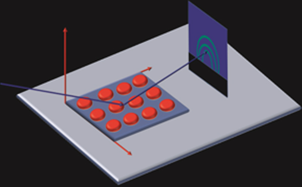
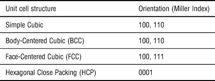
To construct viable CNNs, we created a dataset spanning several million scattering images belonging to seven combinations of unit cells and orientations. HipGISAXS, a high-performance x-ray scattering simulator developed at the Advanced Light Source (ALS), Lawrence Berkeley National Laboratory (LBL), was used to generate the diverse collection of image samples. We simulated scattering patterns of various unit cells with different Miller Indices defining the crystal orientation relative to the substrate. We list the different combinations in Table I. The wavelength used had a photon energy of 10 keV. Simulation time took 500,000 core hours running on the National Energy Research Scientific Computing (NERSC) super computer Edison at LBL. Figure 1 highlights the experimental setup which the simulation captures.
Diagram of experimental setup used in HipGISAXS. The incoming x-ray hits the substrate and scatters off the surface, hitting the detector. The collected image is a reciprocal space representation of the material. This diffraction pattern is simulated in HipGISAXS.

Unit cells and orientations of crystals used in HipGISAXS simulations

We explored a wide parameter space in our simulations to fully assess the robustness of our classification model. During the simulation, we varied experimental variables such as orientation, lattice parameter, and lattice repetition number (defining how many repeating unit cells occurred along each direction). To simulate possible errors in an experimental condition, we incorporated different sources of noise: varying smear effect, Gaussian noise levels, Poisson shot noise, and multiple image resolutions. Only one type of noise was applied to each image at a time with the goal of verifying which noise the trained CNN was most sensitive to.
ML models
Deep learning models have been applied to many classification tasks dependent on pictorial information, frequently using cross-entropy as a loss function.[Reference Goodfellow, Bengio and Courville25] Cross-entropy is defined as the negative log-likelihood of the distribution calculated from the SoftMax function[Reference Nasrabadi26] predicted from deep learning models. It is given by
 $${\rm loss\;} = {\rm \;} -\mathop \sum \limits_{i = 1}^n \mathop \sum \limits_{\,j = 1}^k y_i^j \log p_i^j, $$
where 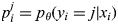 $p_i^j = p_\theta (y_i = j{\rm \vert}x_i)$ is the probability that x i belongs to class j predicted by model θ, and
 $y_i^j $ is the label of the data.
As CNNs provide non-linear models for complex image classification, we constructed a CNN based on the AlexNet architecture,[Reference LeCun, Bottou, Bengio and Haffner11] motivated by AlexNet's previously reported accuracy and relatively low computational requirements. The CNN's input was adapted to accommodate the GISAXS image sizes, and we also adjusted the size of the convolutional layers accordingly. For each type of noise listed previously, we built a dedicated model, and within each noise level, we divided the data into a training and evaluation set with a ratio of 5 to 1. We stratify the data under different directions that are parallel to the thin film substrate to ensure that the ratio of training and evaluation data points are consistent over the different directions. The training of the CNNs was performed on a Tesla P100 GPU server at the ALS. Each model was trained over 20 epochs.
Results and discussion
We initially trained the AlexNet neural network on data obtained through HipGISAXS, unaltered by any additional noise. The training accuracy of the model was 98.57% and the prediction accuracy was 98.12%. Training and prediction accuracies denote the accuracies achieved for training and testing datasets, respectively. The digits in the recorded percentages are significant, since two decimal places represent tens of thousands of images. We also tested two other architectures, VGG-16[Reference Simonyan and Zisserman27] and ResNet-50[Reference He, Zhang, Ren and Sun28] and obtained similar results.
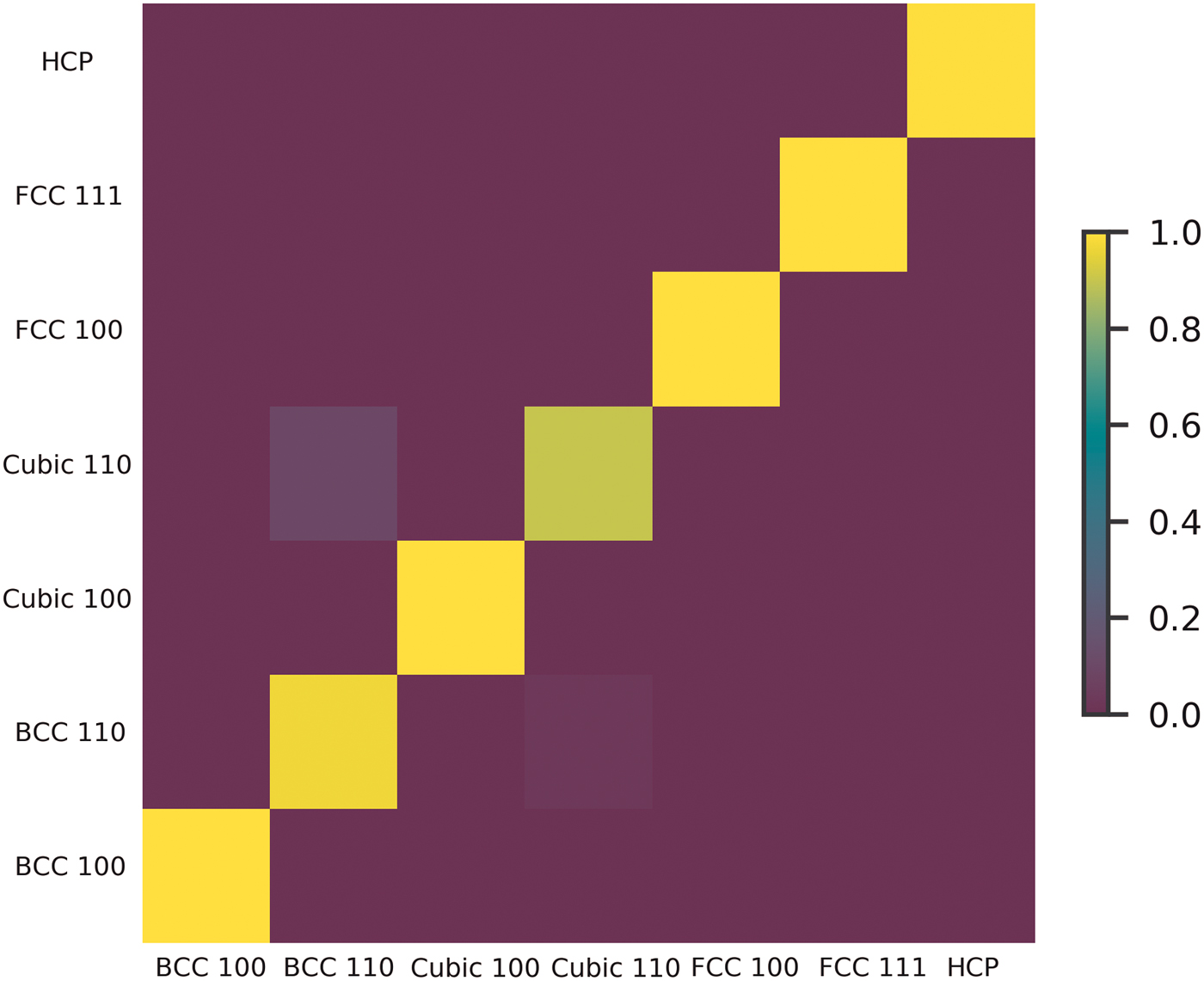
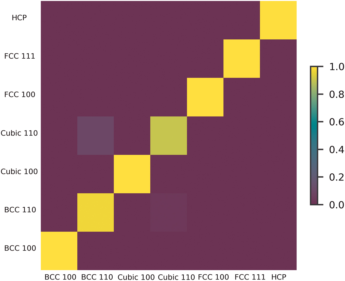
To understand the classification results of the trained CNN, we first calculated the confusion matrix. The elements of the confusion matrix, M i,j, are defined as the ratio of samples with label j classified with label i to the number of samples with label j. The confusion matrix is shown in Fig. 2. Figure 2 highlights confusion in the classification of Simple Cubic 110 and BCC 110. This is attributed to the similarity of the features exhibited in the scattering patterns of different lattices.
Confusion matrix for the trained AlexNet CNN. The confusion matrix highlights the high accuracy of the predictions as shown by the yellow diagonal. The matrix also shows the confusion that exists in classifying Simple Cubic 110 and Body-Centered Cubic 110.
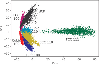
We also visualize the classification method of the CNN by Principle Component Analysis (PCA). Mathematically, we can measure the information carried in principle components using explained variance ratio. The explained variance ratio of the top k components from d dimensional data is defined as
 $${\rm EVR}\; = \; \displaystyle{{\mathop \sum \nolimits_{i = 1}^k \sigma _i^2} \over {\mathop \sum \nolimits_{i = 1}^d \sigma _i^2}}, $$
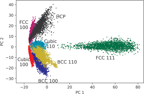
where σ i is the singular value of the i th component. The results of PCA are shown in Fig. 3. Following the confusion matrix, there is a distinct overlap between BCC 110 and Simple Cubic 110. Most interestingly, we noticed a distinct separation between the 100, 110 groups and the 111 group. This highlights the CNN's ability to distinguish between different unit cells and their orientations.
PCA of the final fully connected layer of the AlexNet CNN. PCA shows that there is a clear distinction in the classified 111 unit cells compared with the 100 and 110. We also see the overlap of the Simple Cubic 110 and BCC 110 as was seen in the confusion matrix.

PCA is a powerful tool for data visualization and analysis, but it has also limitations, particularly when the main components represent a small fraction of the data. Here, the first two components only contribute to 65% of the explained variance,[Reference Wold, Esbensen and Geladi29] so classes that seem to be overlapping might be well separated in a higher dimensional space.
As observed in routine x-ray experiments, GISAXS scattering images rarely have sharp features. This can be attributed to multiple factors, such as short-range order in soft matter, imperfections in collimation, non-monochromaticity of the x-ray beam, and different types of read-out noises in the detectors.[Reference Ye, Zhu, Ercius, Raja, He, Jones, Hauwiller, Liu, Xu and Alivisatos30] Mathematically, this effect can be approximated by smearing the images and adding Gaussian noise. The smear effect can be formulated as
 $$\eqalign{I_s(q_x,q_y) &= \displaystyle{1 \over {2\pi \sigma _x\sigma _y}}\mathop \int \nolimits_{-\infty} ^\infty dx\,W(x;0,\sigma _x^2 )\mathop \int \nolimits_{-\infty} ^\infty dy\,W(y;0,\sigma _y^2 )\, \cr & \quad \times I(q_x + x,q_y + y),}$$
where I s and I are the intensity of the beam with and without the smearing effect, respectively, and W(x;μ, σ 2) is a Gaussian distribution with mean μ and variance σ 2. The standard deviations σ x and σ y define the smear scale values. We used equal values for σ x and σ y.
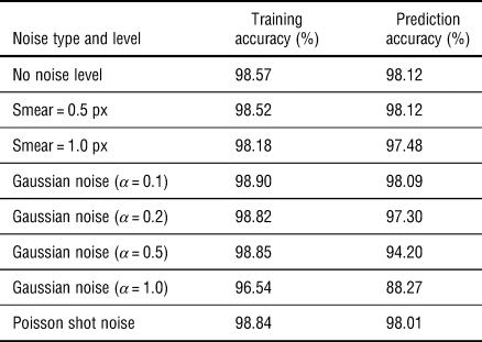
We smeared both the training and test images with different scales to investigate how the smear artifacts affected the training and prediction performances of the AlexNet. The training and prediction accuracies were not affected by small smear scale values (0.5 px). Increasing the smear scale value to 1 px dropped the accuracy down from 98.12% to 97.46%. However, high accuracy was still obtained under different scales, which illustrates the robustness of the deep learning models under the influence of noise.
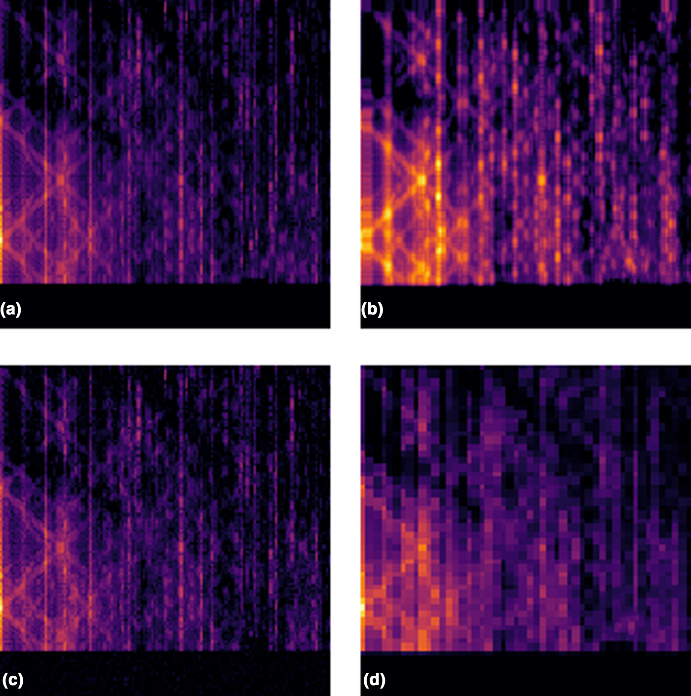
Poisson shot noise can be translated into pixel intensity variations due to the particle distribution in the beam during experiments. Moreover, there can be thermal fluctuations at different pixels of the detector, which can be modeled by a Gaussian distribution of noise. We added Gaussian noise to each pixel and investigated how this error affected the training and testing results of the CNN. The Gaussian noise levels have a mean of zero and a standard deviation given by the multiplication of the Gaussian Noise Level α and the average image intensity I avg. As expected, prediction accuracy decreased with the increased amount of Gaussian noise. When α = 0.2, the prediction dropped to 97.30%. At the highest noise level, a CNN was trained to identify 88.27% of the images successfully. Figure 4 shows an example of how the different noises affect a given simulated scattering image. All the results are tabularized in Table II.
BCC 110 scattering pattern subjected to various noises. (a) Clean data, (b) the data subjected to smear, (c) Gaussian nose, and (d) the data subjected to a lower resolution.

Noise levels and training/prediction accuracies of the trained AlexNet CNNs

As the noise levels are increased, the prediction capabilities of the CNNs decrease.
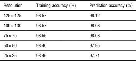
In some cases, GISAXS image resolution is limited by experimental instruments, such as the pixel size of the detector. We scaled our simulated images down to various resolutions and rescaled them back to 125 × 125 using interpolation. The prediction accuracy of the trained models was not heavily affected when the image was scaled to a 50 × 50 resolution. These results indicate that most of the structural information is retained in decreased resolution to allow for successful classification. Scaling the images down to 25 × 25 resulted in a 97.71% prediction accuracy. All the resolutions tested are highlighted in Table III. We conclude that this is due to a vast number of pixels holding little useful information, and even when the resolution was decreased due to a subsampling, the major feature locations and intensities stayed intact.
CNN prediction accuracy as a function of image resolution

The prediction accuracy of the trained CNNs decreases as resolution decreases. Relatively high accuracy is maintained due to maintained feature placement in the downsized image.
We have trained various CNNs on data with different noises. This was done under the assumption that one could identify the noise experienced by the experimental data. In practice, it is not easy to predict how much noise or error will be present in the experiment. We took this into account by taking data that were subjected to high noise levels and had them classified by the CNN that was trained with the data not subjected to any noise.
First, we tested the data subjected to the maximum smear scale. For reference, we are comparing to the testing performance of the AlexNet with no noise: 98.12%. For the highest smear scale, the accuracy dropped to 84.53%. Next, the data with Gaussian noise had a lower accuracy of 62.37%. For a 100 × 100 px image resolution, the accuracy dropped to 97.37%, and for 50 × 50 px resolution, the accuracy dropped to 94.63%. From these results, we found that the ideal CNN model is robust on different noises and circumstances. Among these noises, the model is most vulnerable to Gaussian noise.
Repetition scales
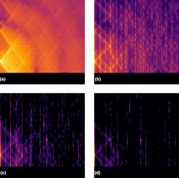
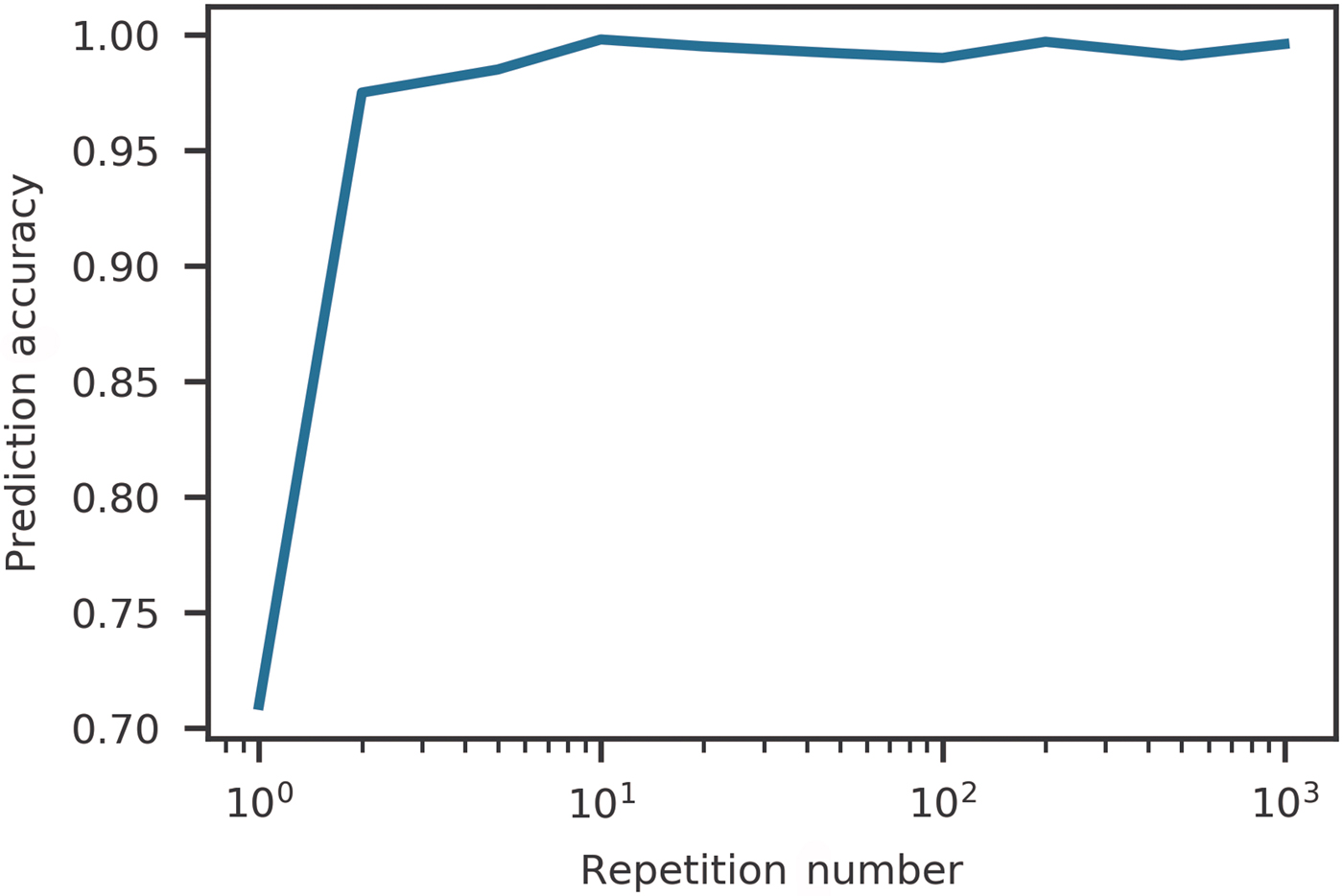
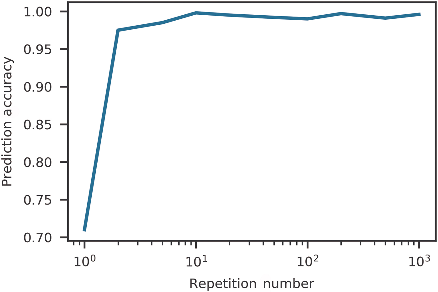
Scattering signals are weakened when crystals have a limited number of repeating units in different directions. To investigate classification for this situation, we generated GISAXS images with various repeating units. Figure 5 highlights how the scattering pattern for a given lattice changes as a function of the number of repeating units of the crystal. We began with a single unit cell and increased the number of repeating units of the crystal equally in two perpendicular directions parallel to the substrate. We kept the number of repetition units in these directions equal. As expected, the prediction accuracy improved with more repetitions. In materials with long range order, the Bragg scattering dominates the diffuse scattering, which enhances the Bragg peaks in the scattering image. The classification success rate as a function of repetition number is shown in Fig. 6.
Effect on a given scattering pattern when the repetition value of the unit cell is changed. Figure (a) shows the limiting case of one unit cell, (b) shows 10 unit cells, (c) shows 100 unit cells, and (d) shows 200 unit cells. We note that the features become more defined as the number of unit cells increase.

CNN prediction accuracy as a function of repeating units in both the x and y directions. The CNN is able to reliably predict the underlying unit cell composing the thin film when there are less than 10 unit cells. This highlights extremely sharp features are not necessarily needed for a reliable prediction by the CNN.
Experimental data classification
We performed a preliminary study to verify the potential of our trained CNN to classify experimental images. We leveraged data acquired from Lawrence Berkeley National Laboratory facilities as described in Ref [Reference Ye, Zhu, Ercius, Raja, He, Jones, Hauwiller, Liu, Xu and Alivisatos30]. That data contain various x-ray diffraction patterns obtained from BCC, HCP, FCC, and Simple Cubic nanoparticle arrays. Access to these data provided us with a unique opportunity to verify our initially trained CNN on real experimental data.
We randomly selected 45 GISAXS images from the dataset and attempted to manually characterize the unit cell and orientation. We confidently identified 33 of the 45 images and passed those 33 images through the trained CNN. The CNN identified the images with a success rate to 52%. According to the proposed analysis, no HCP lattices were identified by the CNN. In Ref. [Reference Ye, Zhu, Ercius, Raja, He, Jones, Hauwiller, Liu, Xu and Alivisatos30], one of the specific lattice types that was manually labeled was HCP. This indicates that the trained CNN lacks the ability to properly identify HCP from various other structures.
Conclusion
In conclusion, we have successfully built an image classification scheme using CNNs for the purpose of classifying various 3D nanoparticle lattice orientations based on simulated and measured x-ray scattering data. Our modified AlexNet was trained on several million images and achieved a training accuracy of over 98%. We introduced various noise sources to the data, such as decreasing the resolution and Poisson noise. When the images were subjected to increased smear and Gaussian noise, the accuracy dropped to 64%. When subjected to a resolution decrease, the image classification accuracy dropped to 94%. We then applied the CNN to a set of real experimental x-ray patterns and predicted the unit-cell classification and orientation with a 52% success rate. We also note that the trained CNN was unable to classify HCP structures.
The use of these trained models on such datasets will highly impact the x-ray and neutron science communities by speeding up GISAXS data analysis of new materials. However, the current predictive models for real data still require improvements to be used in real-world environments. The presented developments will provide guidance for GISAXS users to increase curated public datasets. In future developments, we anticipate to further increase the complexity of the GISAXS model such as different space groups, crystal sizes, and defects in materials, to simulate high complex morphologies and therefore expand the samples this approach can be used for and push towards real-time analysis. Further developments will focus on crystals formed from various materials, different nanoparticle size, and the variation of the form factor by the addition of cylinders. The proposed CNN scheme is very flexible, and it could be extended to other materials such as metal-organic frameworks (MOFs) by constructing simulation data using HipGISAXS and/or by exploiting labeled databases with MOFs experimental data.
Supplementary Material
The supplementary material for this article can be found at https://doi.org/10.1557/mrc.2019.26
Acknowledgments
The authors acknowledge authors Ye, Zhu, Ercius, Raja, He, Jones, Hauwiller, Liu, Xu, and Alivisatos for allowing us to use their data for our real experiment analysis. This work was supported by the Center of Advanced Mathematics for Energy Research Applications (CAMERA) through the Office of Science, of the US Department of Energy under Contract No. DE-AC02-05CH11231 and the Early Career Program. This research is funded in part by the Gordon and Betty Moore Foundation through Grant GBMF3834 and by the Alfred P. Sloan Foundation through Grant 2013-10-27 to the University of California, Berkeley. This research used resources of the National Energy Research Scientific Computing Center (NERSC), a US Department of Energy Office of Science User Facility operated under Contract No. DE-AC02-05CH11231.