1. INTRODUCTION
Many of the main macroeconomic and financial variables across developed countries display significant breaks in unconditional volatility; see, inter alia, Busetti and Taylor (2003), Kim and Nelson (1999), Koop and Potter (2000), McConnell and Perez Quiros (2000), van Dijk, Osborn, and Sensier (2002), Sensier and van Dijk (2004), and references therein. Sensier and van Dijk (2004), e.g., find that over 80% of the real and price variables in the Stock and Watson (1999) data set reject the null hypothesis of constant unconditional innovation variance. Considerable evidence against the constancy of unconditional variances in stock market returns and exchange-rate data has also been reported; cf. Loretan and Phillips (1994). Moreover, Hansen (1995) notes that empirical applications of autoregressive stochastic volatility (SV) models to financial data generally estimate the dominant root in the SV process to be close to the nonstationarity boundary at unity.
Although neither volatility breaks that follow a stationary Markov switching process nor stationary time-varying conditional variances (e.g., autoregressive conditional heteroskedasticity [ARCH]) impact on the large-sample properties of unit root and cointegration tests (for the former, see Nelson, Piger, and Zivot, 2001; Cavaliere, 2003; for the latter, see Hansen and Rahbek, 1998; Kim and Schmidt, 1993; Ling, Li, and McAleer, 2003), permanent changes in volatility can, however, greatly affect unit root inference; see Hamori and Tokihisa (1997), Kim, Leybourne, and Newbold (2002), Cavaliere (2004), and Cavaliere and Taylor (2004). A solution to this problem for the specific case of a single abrupt change in variance is given by Kim et al. (2002), who propose a two-stage procedure where the breakpoint together with the pre- and postbreak variances are first estimated. These estimates are then employed in modified variants of the Perron (1989, 1990) unit root tests. The requirement of a single abrupt change in volatility is, however, not always consistent with empirical evidence, which suggests that data are often better characterized by smooth volatility changes rather than by abrupt changes (see, inter alia, van Dijk et al., 2002) and that multiple changes in volatility are more commonly observed (see, e.g., Watson, 1999). Cavaliere and Taylor (2004) report evidence of multiple volatility breaks and trending volatility in the monthly producer price inflation series from the well-known Stock and Watson (1999) database.
Cavaliere and Taylor (2004) propose a class of modified unit root tests, based on time-transformed data, that are asymptotically robust to a wide class of nonstationary volatility processes that includes multiple and smooth transition breaks. However, because the time transformation involved entails the use of only a subset of the original sample data, simulation results in Cavaliere and Taylor (2004) show that this can lead to significant power losses relative to the corresponding (size-adjusted) standard unit root tests. In this paper we take a different approach and develop bootstrap unit root tests that are, by design, robust to the class of nonstationary volatility considered in Cavaliere and Taylor (2004). We develop bootstrap versions of the autocorrelation-robust M unit root tests of Perron and Ng (1996), Stock (1999), and Ng and Perron (2001), although the approach we outline can equally be applied to any of the commonly used unit root statistics. We focus on the local generalized least squares (GLS) detrended variants of these tests, as favored by Ng and Perron (2001).
Our proposed unit root tests are based on the wild bootstrap method, which replicates in the resampled data the pattern of heteroskedasticity present in the original shocks. An application of the wild bootstrap principle to the problem of estimating stationary autoregressions driven by (stationary) conditionally heteroskedastic errors has recently been shown to perform well by Gonçalves and Killian (2004). As we shall demonstrate, the wild bootstrap unit root statistics share the same limiting null distribution as the original statistics under the class of nonstationary volatility considered. Consequently, inference that is (asymptotically) robust to nonstationary volatility in the shocks can be performed with-out the need to specify any parametric model of volatility within the class considered. Importantly, we show that under local alternatives the bootstrap M tests achieve the asymptotic power functions of (infeasible) size-corrected versions of the standard M tests. We also show that the bootstrap tests are consistent under fixed alternatives.
The paper is organized as follows. In Section 2 we introduce our reference data generating process (DGP) and detail the class of heteroskedastic volatility processes under which we will work. In Section 3 the effects of such nonstationary volatility on the large-sample distributions of conventional unit root tests are discussed. Section 4 develops our heteroskedasticity-robust bootstrap unit root tests and their asymptotic properties. The finite-sample properties of the tests are explored through Monte Carlo simulation in Section 5. Section 6 concludes. All proofs are placed in the Appendix. In the following discussion

denotes weak convergence,

convergence in probability, and

weak convergence in probability (Giné and Zinn, 1990; Hansen, 1996) in each case as the sample size diverges to positive infinity;

is the indicator function and x := y (x =: y) indicates that x is defined by y (y is defined by x); [lfloor ]·[rfloor ] denotes the integer part of the argument,

denotes the space of continuous processes on [0,1], and

denotes the space of right continuous with left limit (càdlàg) processes on [0,1].
2. THE HETEROSKEDASTIC MODEL
Consider the case where we have T + 1 observations generated according to the model


with E(Y02) < ∞. In (1), dt := γ′zt with zt a vector of deterministic components. As in Ng and Perron (2001) we focus on the pth-order trend function, zt := (1,t,…, tp)′, with special focus on the leading cases of a constant (p = 0) and linear trend (p = 1), zt = 1 and zt = (1,t)′, respectively, although the analysis remains valid for more general cases. The following set of assumptions will be taken to hold on (1)–(4).
Assumption

.

The lag polynomial satisfies C(z) ≠ 0 for all |z| ≤ 1, and

.

with E|et|r < K < ∞ for some r ≥ 4.

The volatility term σt satisfies σ[sT] = ω(s) for all s ∈ [0,1], where

is nonstochastic and strictly positive. For t < 0, σt ≤ σ* < ∞.

The autoregressive coefficient α satisfies |α| < 1 or α = 1.
Notice that the error term {ut} in (3) is a linear process in {εt}, the latter formed as the product of two components, {et} and {σt}. Because {et} is independent and identically distributed (i.i.d.), conditionally on σt, the error term εt has mean zero and time-varying variance σt2.
Assumptions

(which states that {ut} has a stable and invertible representation in terms of the εt's and that moments of order four exist; see, e.g., Chang and Park, 2002) and

(which rules out explosive and seasonal unit roots) are standard in the econometric literature. Assumption

is discussed in Remark 1, which follows.
The key assumption for the purposes of this paper is

, which casts the dynamics of the innovation variance in a quite general framework. The class of volatility processes that satisfy Assumption

is extremely wide. Indeed, the innovation variance is required only to be nonstochastic, to be bounded, and to display a countable number of jumps. A detailed discussion of the class of variance processes allowed under

is given by Cavaliere and Taylor (2004), who show that this includes the single abrupt change model of Hamori and Tokihisa (1997) and Kim et al. (2002), variance processes displaying multiple volatility shifts, polynomially (possibly piecewise) trending volatility, and smooth transition variance breaks, among other things.
1The effects of heteroskedastic errors satisfying

on stable autoregressions recently have been analyzed by Phillips and Xu (2006).

, because here ω(s) = σ, for all s.
A quantity that will play a key role in our analysis is given by the following function in

:

Hereafter, η(·) will be referred to as the variance profile of the process, because it depends solely on the time-series behavior of the volatility. Notice that the variance profile satisfies η(s) = s under homoskedasticity, whereas it deviates from s in the presence of heteroskedasticity. Observe also that the quantity

that appears in (5) by Assumption

equals the limit of

and may therefore be interpreted as the (asymptotic) average innovation variance.
Remark 1. Assumption

specifies that {et} is i.i.d. and so consequently rules out processes of major interest such as stationary generalized autoregressive conditionally heteroskedastic (GARCH) or Markov-switching volatility processes. However, it can be shown that the results stated in this paper continue to hold under the weaker condition that for

,

is a martingale difference sequence (MDS) satisfying the following (standard) conditions (see, e.g., Chang and Park, 2002, Assump. 1, p. 433): (a) E(et2) = σe2 = 1, all t; (b)

; and (c) E(|et|r) < K < ∞ for some r ≥ 4, all t. Under this more general framework, et can, e.g., follow a covariance-stationary GARCH process (with finite fourth-order moments) or a stationary Markov-switching volatility process. Consequently, and denoting by ht the conditional variance of et in the MDS case, we can write (4) as

where ht generates (transitory) changes in the conditional volatility and σt generates (permanent) changes in the (un)conditional volatility of εt. This setup therefore includes conditionally heteroskedastic processes with breaks (or trends) in the unconditional volatility, such as in the spline-GARCH model of Engle and Gonzalo Rangel (2004). In what follows, the i.i.d. assumption is maintained, without loss of generality, purely to simplify exposition.
Remark 2. The assumption that the volatility function ω(·) is nonstochastic allows for considerable simplification of the theoretical setup. However, we conjecture that, under suitable memory and moment conditions, this assumption can be weakened to allow for cases where the innovations {et} and ω(·) are stochastically independent. Indeed, in such cases if the (exogenous) volatility process ω(·) has sample paths satisfying Assumption

, then the results presented in the paper can be thought of as holding conditional on a given realization of ω(·). The conditioning argument used here in the context of the volatility function serves the same purpose as the exogeneity assumption used by Perron (1989, pp. 1387–1388) to permit stochastic changes in the trend function. In the (exogenous) SV framework, Markov-switching variances obtain by assuming that ω(·) is a strictly positive, continuous-time Markov chain with a finite number of states, whereas nonstationary autoregressive SV models obtain for ω(s) = h(J(s)), with J(·) a diffusion process in

and h(·) a strictly positive continuous function; see Hansen (1995).
Remark 3. Because the variance σt2 depends on T, a time series generated according to (1)–(4) with σt satisfying Assumption

formally constitutes a triangular array of the type {XT,t := dT,t + YT,t : 0 ≤ t ≤ T,T ≥ 1}, where YT,t is recursively defined as YT,t := αYT,t−1 + C(L)σT,t et, σT,[sT] := ω(s). However, because the triangular array notation is not essential, for simplicity the subscript T is suppressed in what follows.
3. THE M CLASS OF UNIT ROOT TESTS
In this section we outline the M unit root tests of Perron and Ng (1996), Stock (1999), and Ng and Perron (2001) and discuss the impact of time-varying innovation variances on the asymptotic distributions of these statistics.
As in Elliott, Rothenberg, and Stock (1996) denote by

the local GLS residuals from the regression of Xt on zt; i.e.,

, t = 0,…,T, where

is obtained from the ordinary least squares (OLS) regression of

on

and the M unit root statistics are given by

where sAR2(k) is an autoregressive estimator of the (nonnormalized) spectral density at frequency zero of {ut}. Specifically,

where

, i = 1,…, k, and

are, respectively, the OLS slope and variance estimators from the augmented Dickey–Fuller (ADF) regression equation

As is standard, in all of the preceding statistics we require that the lag truncation parameter, k, satisfies the following assumption (Berk, 1974; Said and Dickey, 1984).
Assumption

. As T → ∞, 1/k + k3/T → 0.
In the case of

,

, the unit root null hypothesis (α = 1) is rejected for large negative values of the statistics, whereas a test based on

rejects for small values of the statistic. All three tests are therefore left-tailed. The value of c in (6) and (7) is specified according to the form of the deterministic vector zt and the desired significance level; see Elliott et al. (1996) for details. For p = 0, they suggest c = 7, whereas for p = 1, c = 13.5, in each case for tests run at the 0.05 significance level.
If Assumptions

,

, and

hold on (1)–(4) and σt = σ, t = 1,…,T (so that the errors are homoskedastic), then under the near-integrated autoregressive model, Hc : α := 1 − c/T, with 0 ≤ c < ∞, the asymptotic distributions of the preceding unit root statistics are well known:

where in the constant case (p = 0) Bc0(s,c) = Bc(s), whereas in the linear trend case

, λc := (1 + c)/(1 + c + c2/3), with

, a standard Ornstein–Uhlenbeck process and B(s) a standard Brownian motion; cf. Elliott et al. (1996), Ng and Perron (2001), and Chang and Park (2002).
Representations for the limiting null distributions of the statistics therefore obtain on setting c = 0 in (11). Selected critical values for the tests for p = 0 and p = 1 are provided in Table I of Elliott et al. (1996, p. 825) and Table 1 of Ng and Perron (2001, p. 1524).
For c > 0 the representations can be used to delineate the asymptotic local power functions of the tests, in each case indexed by the noncentrality parameter c. Specifically, for tests run at significance level ε these are given by

where bj(c,p) satisfies P(ξj0,c,p < bj(c,p)) = ε, j = 1,2,3; cf. Elliott et al. (1996, p. 818). Ng and Perron (2001) demonstrate numerically that the

,

, and

tests have asymptotic local power functions each of which is virtually indistinguishable from the local power envelope for both p = 0 and p = 1.
In cases where the volatility process σt is permitted to be generated by any process satisfying Assumption

, we may state the following theorem.
THEOREM 1. Let {Xt}0T be generated as in (1)–(4) under Assumptions

and

and let Hc : α := 1 − c/T, 0 ≤ c < ∞, hold. Then,

,

, and

, where in the constant case (p = 0), Bη,c0(s,c) := Bη,c(s), whereas in the linear trend case

, λc := (1 + c)/(1 + c + c2/3), with

.
As can be seen from the representations given in Theorem 1, the asymptotic null distributions (those pertaining to c = 0) of the unit root statistics have the usual form with the exception that the standard limiting Brownian motion, B0(s), is replaced by the Brownian functional Bη,0(s), the latter reducing to the former only where the process is homoskedastic, i.e., where ω(·) is a constant function. The process Bη,0(s) is known as a variance-transformed Brownian motion, i.e., a Brownian motion under a modification of the time domain; see, e.g., Davidson (1994). This difference has serious implications for the size of the associated unit root tests, with the standard tabulated critical values (cited before) no longer appropriate. The effects of a number of particular variance profiles on the M tests are quantified by Monte Carlo in Section 5.1; see also Hamori and Tokihisa (1997), Kim et al. (2002), and Cavaliere (2004).
It is also clear from the representations in Theorem 1 for c > 0 that the asymptotic local power functions of the tests will also be affected by nonstationary volatility (even if critical values from the correct null distributions were used) because, as with the null case, it is only where ω(·) is constant that the representations given in Theorem 1 reduce to the corresponding representations given in (11). Specifically, the asymptotic local power functions of the tests at significance level ε are given by

where bj(c,p,η) satisfies P(ξj0,c,p,η < bj(c,p,η)) = ε, j = 1,2,3. Moreover, unlike in the homoskedastic case, these cannot necessarily be expected to lie arbitrarily close to the local asymptotic power envelope.
4. BOOTSTRAP UNIT ROOT TESTS
As demonstrated in the previous section, nonstationary volatility introduces a time deformation aspect to the limiting distributions of the unit root statistics under Hc : α = 1 − c/T, which alters their form vis-à-vis the homoskedastic case. In this section we suggest a wild bootstrap algorithm that allows us to retrieve asymptotically correct p-values in the presence of both heteroskedasticity of the form described in Section 2 and serial correlation in the shocks. The wild bootstrap can be successfully implemented in our framework because whereas the asymptotic distributions of the M unit root statistics are affected by the heteroskedasticity-dependent variance profile η(·) under Hc, they are not affected by the short memory properties of the shocks; cf. Theorem 1.
In Section 4.1 we outline our bootstrap algorithm. The asymptotic properties of the bootstrapped M tests are subsequently established in Section 4.2.
4.1. The Bootstrap Algorithm
Let

denote the OLS residuals from the ADF-type regression, (10), based on the local GLS detrended time series

. Next, generate the bootstrap residuals utb according to the device


where {wt}t=1T denotes an independent N(0,1) sequence. In (14) and (15) the multiplicative factor

is what distinguishes the wild bootstrap from a simple parametric bootstrap. It serves to replicate the pattern of heteroskedasticity present in the original shocks in the bootstrap shocks because, conditionally on

, utb is independent over time with zero mean and variance

. The bootstrap sample is then obtained by constructing the partial sum process

for some initial value X0b. Because the asymptotic distributions of the considered tests are not affected by the initial condition as long as E(X0b)2 < ∞ (cf. Section 2), we simply set X0b = 0.
The bootstrap M unit root test statistics, which we will generically refer to as the Mb class of tests, then obtain as follows. Let

denote the local GLS residuals from the regression of Xtb on zt; i.e.,

, t = 0,…,T, where

is obtained from the OLS regression of

on zc; cf. (7). The wild bootstrap analogues of the unit root statistics corresponding to

,

, and

are then computed on the bootstrap sample; i.e.,

and

, where

, where

are the OLS residuals from the regression of

on

(t = 1,…,T). Notice that this is a standard, rather than long-run, residual variance estimator, the bootstrap sample having uncorrelated increments.
The bootstrap p-values finally obtain as

,

, and

, where

,

, and

denote the cumulative distribution functions (c.d.f.s) of

,

, and

, respectively. In practice these c.d.f.s are, of course, unknown and so may be approximated by repeating the wild bootstrap resampling procedure a large number of times; cf. Hansen (1996) and Andrews and Buchinsky (2001). Specifically, and taking the

statistic to illustrate, from the doubly independent N(0,1) sequence{{wj,t}t=1T}j=1N, N conditionally independent bootstrap statistics

, j = 1,…, N, are computed as before but from

,

, t = 1,…,T. The simulated bootstrap p-value is then computed as the percentage of bootstrap statistics that do not exceed the actual statistic; i.e.,

. Note that an asymptotic standard error for

is given by

; cf. Hansen (1996, p. 419). Applying the same approach to the

and

statistics yields the corresponding quantities

and

.
Remark 4. Although, as mentioned previously, the bootstrap statistics do not require a long-run variance estimator, one could equivalently construct the bootstrap p-values by using the statistics

and

, where sARb(kb)2 is the long-run variance estimator

with

, i = 1,…, kb, and

the OLS slope and variance estimators, respectively, from a standard ADF regression on

using kb lags. Because the bootstrap sample has uncorrelated increments, kb in (19) need not diverge to infinity with T, unlike k in (9). Notice that

.
Remark 5. In principle, the bootstrap integrated time series (16) does not need to be generated by using the residuals from an ADF regression based on local GLS detrended data. For example, one could obtain the residuals by imposing a unit root in the data. This procedure would not alter the large-sample properties of the bootstrap procedure. More specifically, the asymptotic properties of the wild bootstrap do not change if

of (14) is alternatively defined through any one of the following procedures:
(a)

, the residuals from a standard k-lags autoregression run on

using k lags (i.e., by imposing a unit root);
(b)

, the residuals from a simple Dickey–Fuller regression on the local GLS detrended data, i.e., of

on

;
(c)

, obtained by differencing the local GLS detrended data, i.e.,

;
(d) ut0, obtained as Xt − Xt−1, corrected for Δzt.
Although the large-sample properties of the wild bootstrap are not affected by the choice of

, numerical evidence suggested that procedure (d) delivered the best finite-sample size and power properties of the five suggested procedures.
Remark 6. As is well known in the wild bootstrap literature (for a review, see Davidson and Flachaire, 2001) in certain cases better bootstrap accuracy can be obtained by replacing the Gaussian distribution used for generating the pseudo-data by an asymmetric distribution with E(wt) = 0, E(wt2) = 1, and E(wt3) = 1 (Liu, 1988). A well-known example of this is the Mammen (1993) two-point distribution:

,

. We found no discernible differences between the finite-sample properties of the bootstrap unit root tests based on the Gaussian or Mammen distribution.
4.2. Asymptotic Properties
In this section we discuss the asymptotic properties of the wild bootstrap unit root tests. We show that under the unit root null, and for any volatility process satisfying Assumption

, the bootstrap statistics converge to the same asymptotic distribution as the test statistics computed on the original data; i.e., the wild bootstrap allows us to replicate the correct first-order asymptotic null distribution of the test statistics of interest. We also demonstrate the asymptotic properties of the bootstrap statistics under both near-integrated and stable autoregressive alternatives.
Recall from Section 2 that in the presence of nonstationary volatility satisfying Assumption

,

,

, and

denote the asymptotic distributions of

,

,

, respectively, under Hc : α = 1 − c/T. The usefulness of the wild bootstrap in the present framework is given in the following result, which shows that our bootstrap procedure allows us to retrieve the correct asymptotic null distribution and hence that the p-values based on

,

, and

are all asymptotically pivotal.
THEOREM 2. Let the conditions of Theorem 1 hold and let the bootstrap sample be generated as detailed in Section 4.1. Then

,

, and

. Moreover, if α = 1,

,

, and

.
Theorem 2 proves the usefulness of the wild bootstrap under the null hypothesis: as the number of observations diverges, the bootstrapped statistics have the same null distribution as the original test statistics, and consequently the bootstrap p-values are uniformly distributed under the null hypothesis, leading to tests with asymptotically correct size. As Theorem 2 also shows, these limiting distributions also hold for the bootstrapped statistics under local alternatives. This immediately implies that the bootstrap unit root tests will have the same asymptotic local power functions as the original unit root tests, provided the latter were run using critical values from the appropriate limiting null distribution, i.e., the asymptotic local power functions given in (13). The asymptotic theory therefore predicts that the bootstrap tests should have power approximately equal to the size-adjusted power of the standard tests.
We now turn to the behavior of the bootstrap statistics under stable autoregressive alternatives. The distribution of the bootstrap statistics is derived under the assumption that α of (2) is bounded by |α| < 1, and it is shown that, as a result, our bootstrap unit root tests are consistent.
THEOREM 3. Let {Xt}0T be generated as in (1)–(4) under Assumptions

and

, with |α| < 1, and let the bootstrap sample be generated as in Section 4.1. Then,

,

,

. Moreover,

and

diverge to minus infinity whereas

; hence,

,

,

.
The finite-sample behavior of the standard and bootstrap M tests is explored in the next section.
5. FINITE-SAMPLE SIMULATIONS
In this section we analyze the finite-sample size and power properties of the bootstrap Mb unit root tests of Section 4 by means of Monte Carlo simulation. Precisely, the

,

, and

tests are considered and compared with the standard

,

, and

tests. Results are presented for the constant (p = 0) case. Results for the linear trend (p = 1) case are qualitatively similar and are available on request.
We generated data according to (1)–(4), with X0 = 0, for samples of size T = 100, 250, and 500 with et ∼ IN(0,1), using the Kiss+Monster function of Gauss 5.0. All experiments were conducted using 10,000 Monte Carlo replications. The standard M tests were computed as in (8) and were run using the nominal asymptotic 0.05 level critical values appropriate for the homoskedastic case. The bootstrap Mb tests were constructed as outlined in Section 4 with kb = k, using the first difference residual bootstrap (scheme (d) outlined in Remark 5) and Gaussian pseudo-data. The number of bootstrap replications used was N = 499 throughout.
Initially, and to demonstrate the effects of heteroskedasticity on the finite-sample size (Section 5.1) and power (Section 5.2) properties of the standard M and corresponding bootstrap Mb tests uncontaminated by the separate effects of serial dependence, we set C(L) = 1 in (3), so that the error term ut = σt et. Correspondingly, we set k = 0 in (9) and kb = 0 in (19). In Section 5.3 we extend the analysis to also allow for weak dependence in ut, reporting results for a subset of the cases reported in Sections 5.1 and 5.2.
Results are reported for the following four models for the time-series behavior of the volatility term σt2:
A. Single volatility shift. A single abrupt shift in volatility from σ02 to σ12 occurring at time [lfloor ]τT [rfloor ], which corresponds to the variance function

with τ ∈ (0,1).
B. Two volatility shifts. Two volatility shifts, the first from σ02 to σ12 occurring at time [lfloor ]τ1T [rfloor ], the second from σ12 to σ02 occurring at time [lfloor ]τ2T [rfloor ], which corresponds to the variance function

for τ1,τ2 ∈ (0,1), τ1 < τ2.
C. Trending volatility. Volatility follows a linear trend, between σ0 for t = 0 and σ1 for t = T, which corresponds to the volatility function

D. Exponential (near-) integrated stochastic volatility. Standard models of (near-) integrated SV can be approximated through the variance function (see the discussion in Hansen, 1995, p. 1116),

for ν > 0, with Jc(·) either an Ornstein–Uhlenbeck process (c > 0) or a Brownian motion (c = 0).
Without loss of generality we set σ02 = 1 in all cases. For Model A we let the ratio δ := σ0 /σ1 vary among

, and the break date among τ ∈ {0.1, 0.9}, so that both early and late breaks, which may be positive (δ < 1) or negative (δ > 1), are allowed. For Model B we vary the ratio δ := σ0 /σ1 among

and consider symmetric shifts, such that τ2 = 1 − τ1, with τ ∈ {0.05, 0.45}, thereby allowing for breaks that occur either toward the middle or the start and end of the sample. For Model C we let δ := σ0 /σ1 take values among

so that both positively and negatively trending variances are generated. Finally, for Model D we vary ν among {4, 9} and c among {0, 10, 20}. It should stressed that, formally, Model D does not satisfy Assumption

; however, see Remark 2.
For each of Models A–D other combinations of parameter values were also considered, including asymmetric shifts in the case of Model B, but these qualitatively add little to the reported results. In the case of Models A and B we also considered smooth (logistic) transition shifts in variance. These results were qualitatively similar to those reported subsequently, with the effects of the volatility breaks diminishing somewhat as the speed of transition parameter is reduced, other things being equal, as would be expected. We also considered the cases where the volatility process follows either a covariance stationary autoregressive SV process of the form σt2 = σ02 exp(νht), ht = γht−1 + et, or a covariance stationary autoregressive conditionally heteroskedastic GARCH(1,1) process of the form σt2 = α0 + α1εt−12 + β1σt−12 where in both cases et is as before. In each case, both the standard and bootstrap tests behaved almost identically to the constant volatility case here, as expected; cf. Remark 1. All of these results are available on request.
5.1. Size Properties
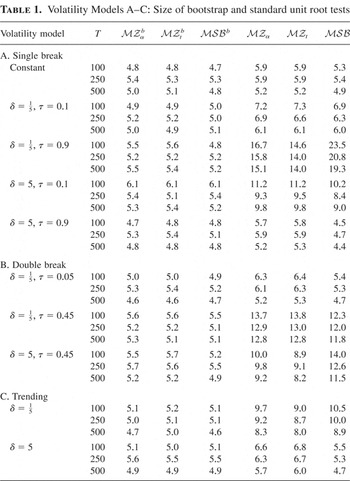
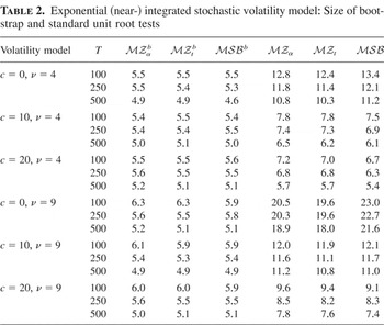
Tables 1 and 2 present the (empirical) size, for α = 1 in (2), of both the standard M unit root tests and the corresponding Mb heteroskedastic-robust bootstrap unit root tests of Section 4.
Volatility Models A–C: Size of bootstrap and standard unit root tests

Exponential (near-) integrated stochastic volatility model: Size of bootstrap and standard unit root tests

Let us initially consider the single break model (Table 1A). As for the unit root tests considered by Kim et al. (2002) and Cavaliere (2004), the standard M unit root tests are badly oversized in the presence of early negative and late positive breaks. For example, the

statistic shows empirical size of around 20% in the presence of late positive breaks. In contrast, the size properties of our Mb bootstrap unit root tests seem largely satisfactory throughout. It is also worth noting that in the homoskedastic case, the bootstrap yields tests with finite-sample size closer to the nominal level than the standard tests based on asymptotic critical values.
The results for the double volatility break model (Table 1B) are broadly comparable to those obtained for the single break model. As far as the standard M tests are concerned, the most severe size biases are seen for a positive followed by a negative break, both occurring toward the middle of the sample (actual size varies between around 12% and 15%), whereas a negative followed by a positive break again toward the middle of the sample also causes significant oversizing in the standard tests. Conversely, our proposed Mb tests perform well, completely avoiding the oversizing problems seen with the standard M tests.
The results in Table 1C show that, in general, linear trending volatility has a lower impact on the size of the standard tests than abrupt changes. The M tests are notably oversized for p = 0 (around 10% size) in the presence of upward trending volatility

. Downward trending volatility (δ = 5) appears to have rather less impact. Again the Mb tests display empirical sizes very close to the nominal level throughout.
The size properties of the tests in the presence of (near-) integrated volatility are reported in Table 2. In the “mildest” case, when ν is low (ν = 4) and volatility is strongly mean reverting (c = 20), the standard M tests perform well in terms of size, which is rarely in excess of 7%. However, when ν grows and/or c decreases, the impact of volatility becomes more pronounced, leading to strongly oversized tests. When the volatility is nonstationary (c = 0) and ν is low, the rejection frequencies of the standard unit root tests range between about 8% and 14%. When ν is high, such frequencies all but double. Significant oversizing is also seen when ν is high but the process is mean reverting (c = 10,20). The performance of the Mb tests is very good, with empirical size never in excess of 6.5%, supportive of our conjecture in Remark 2.
5.2. Power Properties
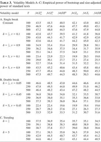
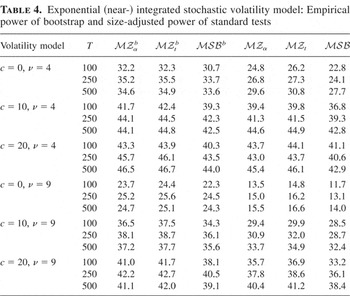
Tables 3 and 4 report the finite-sample powers of the bootstrap Mb unit root tests of Section 4, together with the (size-adjusted) powers of the corresponding standard M unit root tests. The reported results are for the same models as considered in Section 5.1 except that we replace α = 1 with the local alternative α = 1 − 7/T in (2). Under constant volatility, therefore, power would be expected to be close to 50%, and this should be viewed as the relevant benchmark when reading the results. Qualitatively similar conclusions were drawn for other values of α. In the case of the standard M tests size-adjusted power is reported to control for the unreliable size properties of these tests under nonstationary volatility; see Section 5.1.
Volatility Models A–C: Empirical power of bootstrap and size-adjusted power of standard tests

Exponential (near-) integrated stochastic volatility model: Empirical power of bootstrap and size-adjusted power of standard tests

Consider first the case where the errors are homoskedastic, which is reported in Table 3A. Here the bootstrap Mb tests display roughly the same power as the corresponding standard M tests. Hence, appealingly, the bootstrap does not appear to lead to any significant power loss when the data are homoskedastic.
Under heteroskedasticity (Tables 3 and 4) the standard M tests tend to experience a decrease in size-adjusted power, relative to the constant volatility case, in cases where the tests are significantly oversized under the null. This effect can be most clearly seen in the single break model with a late positive break or early negative break, in the double break model where a positive followed by a negative break or a negative followed by a positive break occur toward the middle of the sample, and in the (near-) integrated volatility case when either c = 0 or ν is large. As anticipated by the asymptotic theory (see the discussion after Theorem 2), the bootstrap Mb tests display power that is very similar to the size-adjusted power of the corresponding M tests throughout. The only exception seems to be the case of integrated volatility (c = 0), especially when ν is large, where the Mb tests display power somewhat in excess of the size-adjusted power of the corresponding M tests.
Overall, our bootstrap Mb tests perform very well in practice. They all but eliminate the serious size distortions seen with the standard M tests across a range of models of nonstationary volatility, yet display almost identical finite-sample power properties to (infeasible) size-adjusted M tests under near-integrated alternatives.
5.3. Serial Correlation
Consider now the case where we allow for both nonstationary volatility and serial dependence in the shocks, so that C(L) ≠ 1 in (3). Because serial correlation is now permitted the M and Mb tests are constructed as detailed at the start of this section except that now, as in Ng and Perron (2001, p. 1536), we set the maximum lag k = kb = [lfloor ]12(T/100)1/4[rfloor ] in (9) and (19). The preferred modified Akaike information criterion (MAIC) lag selection criterion of Ng and Perron (2001) was employed throughout. We also computed the corresponding experiments for kb = 0: these results were little different from those reported.
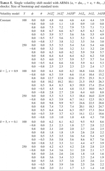
Table 5 reports the size of the M and Mb tests with data-dependent lag selection for data generated as outlined at the start of this section with α = 1, but where the errors are now generated according to either an MA(1) process, i.e., ut = εt + θεt−1, or an AR(1) process, i.e., ut = φut−1 + εt so that C(L) = (1 + φL + φ2L2 + …), in (3). The moving average parameter θ was chosen within the set {0, ±0.5, ±0.8}, and the autoregressive parameter within the set {0, ±0.8}. For space constraints results are reported for two of the volatility models, namely, the constant volatility and late negative single volatility shift (

, τ = 0.9) models,
2Corresponding experiments were conducted for the other models of nonstationary volatility considered in Sections 5.1 and 5.2, but qualitatively these neither added to nor contradicted the reported results.
Single volatility shift model with ARMA (ut = φut−1 + εt + θεt−1) shocks: Size of bootstrap and standard tests

Consider first the results for the constant volatility model in Table 5. Here we can compare the finite-sample performance of the bootstrap Mb and corresponding standard M tests in the presence of serially correlated shocks. Overall there is really little to choose between the standard and bootstrap tests. Both do, overall, an excellent job in controlling size. However, consistent with the findings of Ng and Perron (2001), significant undersize is seen for the large negative autoregressive model (φ = −0.8) and for the large negative moving average model (θ = −0.8), whereas some oversize is seen with the large positive autoregressive model (φ = 0.8) and to a lesser extent positive moving average models.
Turning to the nonstationary volatility model, we see that for the standard M tests the size distortions observed for this case with serially uncorrelated shocks in Table 1 and the size distortions noted previously for the serially correlated but homoskedastic case appear to combine. In general the oversize due to the nonconstant variance process is further increased in cases where the serial correlation in the shocks causes oversize: this is particularly pronounced in the case of either large positive autoregressive (φ = 0.8) or moving average (θ = 0.8) models. The reverse holds true for cases where serial correlation causes undersizing. The bootstrap Mb tests are much less badly affected than the standard tests, although significant finite-sample oversize is again seen for the large positive autoregressive and moving average models. These distortions are, however, significantly reduced between T = 100 and T = 250, as predicted by the asymptotic theory.
6. CONCLUSIONS
The presence of nonstationary volatility has potentially serious implications for the reliability of unit root tests, affecting tests whose true size can be significantly in excess of the nominal significance level. To rectify this problem, we have proposed a wild bootstrap–based approach to testing for a unit root. Unlike previous tests that have appeared in the literature, our approach requires only that the innovation volatility is nonstochastic, is bounded, and has a countable number of jumps. Our proposed bootstrap unit root tests have the considerable advantage that they are not tied to a given parametric model of volatility within the class of nonstationary volatility processes considered. This is a particularly attractive feature because economic and financial series appear to be subject to both smooth volatility changes and multiple volatility changes, the break dates associated with which can be hard to identify in practice. As with any bootstrap procedure, no tables of critical values are required as the procedure automatically delivers a p-value for the hypothesis being tested. The asymptotic validity of our proposed bootstrap tests within the class of nonstationary volatility considered was demonstrated. Monte Carlo evidence was also reported that suggested that the proposed bootstrap unit root tests perform well in finite samples, avoiding the large oversize problems that can occur with the standard tests in the presence of a variety of forms of nonstationary volatility, yet emulating the finite-sample power properties of (infeasible) size-adjusted implementations of the standard tests.
Although the class of nonstationary volatility processes considered in this paper is wide, containing many of the forms of nonstationarity argued for in the empirical literature, we have imposed the condition that the volatility process is nonstochastic. We conjecture that the wild bootstrap–based unit root tests outlined in this paper will remain asymptotically valid in the presence of (exogenous) stochastic volatility under suitable moment and memory conditions. A proof of this conjecture is beyond the scope of the present paper but is currently under investigation by the authors. Monte Carlo results presented in the paper for the empirically important case of near-integrated autoregressive stochastic volatility appeared supportive of our conjecture.
MATHEMATICAL APPENDIX
In the following discussion we assume that γ = 0 without loss of generality. Some of the proofs are based on the following lemmas. More specifically, in Lemmas 2 and 3 two uniform consistency results for the squared residuals

from (10) are given.
LEMMA 1. Let

and let

. Then, under Assumption

, as T → ∞, and uniformly for all j = 0,…, k = o(T): (i)

and (ii)

, where

denotes convergence in L2 as T → ∞.
Proof. The proof is similar to the proof of Lemma 3 in Cavaliere and Taylor (2007) and is therefore omitted in the interest of brevity. █
LEMMA 2. Let the conditions of Theorem 1 hold. Then,

uniformly for all s ∈ [0,1].
Proof of Lemma 2. We assume, without loss of generality (see Chang and Park, 2002; Park, 2003), that c = 0 and that the residuals

are obtained under the null hypothesis, i.e., by estimating the regression

. In this case, if

is replaced by Xt, so that the estimated regression is

, in Cavaliere and Taylor (2007) it is shown that

. We now generalize this result to the case of local GLS residuals. Initially, we show that the difference between

(where

,

, with xt,k := (ΔXt−1,…, ΔXt−k)′ = (ut−1,…,ut−k)′) and the estimator based on the residuals

from the local GLS projection of Xt on Xt−1,

(where

,

, with

), satisfies

under Assumption

, where ∥·∥ denotes the (matrix) euclidean norm. (That is for a matrix A, ∥A∥ := sup∥x∥<1∥Ax∥, using the euclidean norm for the vector x, i.e., ∥x∥2 := x′x.) As

and

are bounded in probability, as shown in Cavaliere and Taylor (2004), this result follows from the inequality

, if we can prove the sufficient conditions: (a)

and (b)

. To see that (a) holds, as in Berk (1974, p. 493), set

,

,

so that

, which implies q ≤ p2Q/(1 − pQ) for pQ < 1. As

, q → 0 in probability if Q = op(1). To prove the last condition, note that

; under local GLS demeaning, Δdt = 0, and hence Q = 0, as expected; under local GLS linear detrending,

(see the proof of Theorem 2, which follows); furthermore, using supt|ut| = op(T1/2), we easily obtain Q2 = op(k2/T) → 0 under

. For (b), similarly to (a),

.
Having established that

, it is straightforward to see that the residual-based estimators

and

converge in probability to the same limiting functional. By Lemma A.10 of Hansen (2000a) the convergence is also uniform over all s ∈ [0,1], because

is monotonically increasing in s and the limit function is continuous (see also Hansen, 2000b, p. 112). █
LEMMA 3. Let the conditions of Theorem 3 hold. Then

uniformly for all s ∈ [0,1].
Proof of Lemma 3. Under the conditions of Theorem 3, the process may be written as

; as |α| < 1, it is straightforward to see that

also implies the summability condition

. Moreover, the process admits the AR(∞) representation

which can be approximated through the (k + 1)th order autoregression (for the homoskedastic case, see Chang and Park, 2002):

with (β1,∞*,…, βk+1,∞*)′ =: βk*. Assume, for the present, that the auxiliary ADF regression (10) is estimated using Xt instead of the local GLS detrended series

. As in Lopez (1997), the residuals from (10) coincide with the OLS residuals from (A.2), say,

Hence, using the results in Cavaliere and Taylor (2007, proof of Thm. 1(ii)), it is straightforward to obtain that under nonstationary heteroskedasticity

; cf. Chang and Park (2002) for the homoskedastic case.
Let us define the following functionals on [0,1]:

,

, where xt,k* := (Xt−1,… Xt−k−1)′. Now, observe that

and consider the equality

We now show that g1(s) and g2(s) are both of op(1). Regarding g1(s), consider the inequalities

As demonstrated previously,

. Moreover, because

, with Mxx,k* = ωT,k2(1)Fk*, ωT,k2(1) as defined in Lemma 1, and

,

, we obtain

as

(see Cavaliere and Taylor, 2007) and ∥Mxx,k*∥ = ωT,k2(1)∥Fk*∥ = O(1) (the last equality following from ωT,k2(1) being bounded and from ∥Fk*∥ being of O(1) under the stated assumptions; cf. Berk, 1974). Hence, ∥g1(s)∥ = op(k−1) uniformly for all s in [0,1].
Results for g2(s) follow similarly. Specifically, because

where

and

(see Cavaliere and Taylor, 2007), the desired result immediately follows.
Because

, to prove the lemma it is left to be shown that

, uniformly. As

(cf. Chang and Park, 2002), pointwise convergence follows straightforwardly using Lemmas 1 and 2 in Cavaliere and Taylor (2007). The proof that the convergence is also uniform then follows using the same arguments as were employed in the proof of Lemma 2.
Finally, tedious but straightforward algebra allows us to show that the preceding results also hold if

is based on the residuals of the local GLS projection of Xt on zt. █
Proof of Theorem 1. The theorem can be proved by extending the proof of Theorem 1 in Cavaliere and Taylor (2007) to the case of local GLS detrended data. This extension is straightforward and is therefore omitted for brevity. █
Proof of Theorem 2. Recall from Section 4 that the bootstrap time series Xtb satisfies

, s ∈ [0,1]. Because {wt} is Gaussian, then, conditionally on

, T−1/2X[lfloor ]sT [rfloor ]b is Gaussian with covariance kernel

, where

. Using Lemma 2, we have the result that

uniformly for all s. Furthermore, ω2η(s) is the kernel function of the variance-transformed Brownian motion ωBη(s) = ωB(η(s)), which implies the weak convergence in probability result

Note that this convergence holds irrespective of the value taken by the local-to-unity noncentrality parameter, c. Standard continuous mapping arguments then apply to the convergence (A.4), implying, e.g., the following results:


jointly. We now establish a weak convergence in probability result for the local GLS detrended series

. Let

Suppose p = 0 first. In this case, zc′zc → 1,

by (A.5) and (A.6). Hence,

and

Consider next the case p = 1, i.e., zt = (1,t)′, and note that

, where δT := diag(1,T). Obviously,

. As in Elliott et al. (1996), (δT−1zc′zcδT−1) → diag(1,1 + c + c2/3), and, after some algebra based on (A.4) and (A.8), one obtains that

The latter result implies that

, from which it follows that

. This establishes that the local GLS residuals,

, obtained from the regression of Xtb on zt, satisfy the weak convergence in probability result,

. Consequently, from a standard continuous mapping argument,

Now consider the bootstrap residual variance estimator,

, which can be written as

where

. Consider first

. It is straightforward to see that for p = 0,

, whereas, for p = 1, we may write

. In the latter case, because

is of Op(T1/2) and

(see the preceding discussion),

and

are both of op(1). Hence, provided that

we immediately have the result that

as required. To establish the validity of (A.12) consider the following equality:

with ξt := wt2 − 1 an independent sequence of centered χ2(1) random variables and f1,f2 implicitly defined. By Lemma 2,

. Moreover, conditionally on the sample,

because

is of Op(1) under E(et4) < ∞.
Now, consider the random variable

, which can be written (see, e.g., Phillips, 1987; Stock, 1994) as

. By using (A.10), (A.13), and a continuous mapping argument we obtain that

which, taken together with (A.6), yields the result that

. Hence, from (A.11) we have that

, which, taken together with (A.10), yields that

This result also implies that, uniformly in probability,

, with

denoting the c.d.f. of

, i = 1,…,3. This implies that under the null hypothesis

converges weakly to U [0,1].
The remainder of the proof is identical to the proof of Theorem 5 in Hansen (2000b). The corresponding results for

and

follow similarly. █
Proof of Theorem 3. We first need to establish that the bootstrap statistics have the same asymptotic distribution as under the null hypothesis. This result will also imply that, uniformly in probability, the c.d.f.s of

,

, and

, say,

,

,

, satisfy

,

,

. This result can be shown by following exactly the same steps as in the proof of Theorem 2, with the only difference that now we need to call Lemma 3, which is designed for fixed alternatives, instead of Lemma 2, which is valid under the null hypothesis and local alternatives.
It is left to prove that, under the conditions of the theorem,

and

diverge to negative infinity whereas

converges to zero, in each case as the sample size diverges. By adapting Stock (1999) to the present framework, a sufficient condition for

,

and

is that TsAR2(k) diverges as T → ∞. We now prove that this requirement holds by showing that 1/(TsAR2(k)) converges to zero in probability. As in the proof of Lemma 2 we clarify exposition by assuming, without loss of generality, that the auxiliary ADF regression, (10), is estimated using Xt instead of the local GLS detrended series

.
First, notice that the OLS estimates from (10) are related to those from the AR(k + 1) regression (A.3) via

and

, i = 1,…, k. Consequently, because

, sAR2(k) may be written as

with ck := (1,2,…, k)′, and, hence,

Using the results in the proof of Lemma 2, and because

, we have

, which implies that

. It is also easy to verify that ck′ βk* is bounded; specifically,

implies that the coefficients of autoregressive representation (A.1) satisfy

(see Chang and Park, 2002, p. 434, and references therein). This condition suffices for

to be bounded as k diverges. Hence, the numerator in (A.14) is bounded in probability. Finally, because from the proof of Lemma 3 we know that

, we obtain that

.
It then follows immediately that

,

, and

, which completes the proof of the theorem. █