



1 Introduction
The impact of flexibility on propulsion has been the focus of research in many different biological systems, such as swimming jellyfish (Demont & Gosline Reference Demont and Gosline1988; Megill, Gosline & Blake Reference Megill, Gosline and Blake2005; Colin et al. Reference Colin, Costello, Dabiri, Villanueva, Blottman, Gemmell and Priya2012; Hoover & Miller Reference Hoover and Miller2015; Hoover, Griffith & Miller Reference Hoover, Griffith and Miller2017), swimming lamprey (Tytell et al. Reference Tytell, Hsu, Williams, Cohen and Fauci2010; Tytell, Hsu & Fauci Reference Tytell, Hsu and Fauci2014; Hamlet, Fauci & Tytell Reference Hamlet, Fauci and Tytell2015; Tytell et al. Reference Tytell, Leftwich, Hsu, Griffith, Cohen, Smits, Hamlet and Fauci2016) and flying insects (Miller & Peskin Reference Miller and Peskin2009). In addition, Leftwich et al. (Reference Leftwich, Tytell, Cohen and Smits2012) examined the effect of a flexible tail on the swimming performance of a robotic lamprey. Other studies use simplified physical models, where a flexible hydrofoil or panel takes the place of an animal’s flexible appendage (Alben et al. Reference Alben, Witt, Baker, Anderson and Lauder2012; Dewey et al. Reference Dewey, Boschitsch, Moored, Stone and Smits2013; Paraz, Eloy & Schouveiler Reference Paraz, Eloy and Schouveiler2014). Most of these studies analyse the propulsive performance of a tethered panel whose leading edge is driven in a periodic motion in a flow tank (Dewey et al. Reference Dewey, Boschitsch, Moored, Stone and Smits2013). In these studies, the experimental set-up is adjusted to examine the effects of many different factors, such as the elastic properties of the panel (Quinn, Lauder & Smits Reference Quinn, Lauder and Smits2014b ; Lucas et al. Reference Lucas, Thornycroft, Gemmell, Colin, Costello and Lauder2015), panel geometries (Buchholz & Smits Reference Buchholz and Smits2006, Reference Buchholz and Smits2008; Green, Rowley & Smits Reference Green, Rowley and Smits2011), the motion of the leading edge (Hover, Haugsdal & Triantafyllou Reference Hover, Haugsdal and Triantafyllou2004; Licht et al. Reference Licht, Wibawa, Hover and Triantafyllou2010; Lehn et al. Reference Lehn, Thornycroft, Lauder and Leftwich2017) and wall effects (Quinn, Lauder & Smits Reference Quinn, Lauder and Smits2014a , Reference Quinn, Lauder and Smits2015). Other simplified models examine the hydrodynamics of free-swimming panels with flexibility localized to a torsional spring present at the leading edge (Alben & Shelley Reference Alben and Shelley2005; Vandenberghe, Childress & Zhang Reference Vandenberghe, Childress and Zhang2006; Spagnolie et al. Reference Spagnolie, Moret, Shelley and Zhang2010; Ramananarivo, Godoy-Diana & Thiria Reference Ramananarivo, Godoy-Diana and Thiria2011).
The motivation of many of these studies has been the potential benefits of biomimetics in engineering. Recent advances in biologically inspired underwater vehicles have given an impetus to understanding the role of flexibility in enhancing their swimming performance (Colin et al. Reference Colin, Costello, Dabiri, Villanueva, Blottman, Gemmell and Priya2012; Raj & Thakur Reference Raj and Thakur2016). For vehicles that are propelled with the actuation of flexible propulsors, understanding the role of mechanical resonance can yield insight into design of the vehicle and an optimized pattern of actuation (Chu et al. Reference Chu, Lee, Song, Han, Lee, Kim, Kim, Park, Cho and Ahn2012). By examining these problems from a modelling perspective, we can shed light on the limitations and constraints that have shaped biological organisms and how these can inform future vehicle design (Fish & Beneski Reference Fish, Beneski and Goel2014).
In addition to physical models, computational models have been developed to investigate the fluid mechanics of flapping propulsion. In many cases, the role of flexibility in propulsion is not considered fully and the kinematics of the swimmer is prescribed (Dong, Mittal & Najjar Reference Dong, Mittal and Najjar2006; Borazjani & Sotiropoulos Reference Borazjani and Sotiropoulos2008, Reference Borazjani and Sotiropoulos2009). Other studies account for the flexibility of the panels in the motion of the leading edge, but not the body itself (Eldredge, Toomey & Medina Reference Eldredge, Toomey and Medina2010; Spagnolie et al. Reference Spagnolie, Moret, Shelley and Zhang2010; Moore Reference Moore2014, Reference Moore2015). Models that employ inviscid fluid assumptions must take steps to account for vorticity generated by the fluid–structure interface (Liu & Bose Reference Liu and Bose1997; Alben Reference Alben2008; Michelin & Llewellyn Smith Reference Michelin and Llewellyn Smith2009; Alben et al. Reference Alben, Witt, Baker, Anderson and Lauder2012; Moore Reference Moore2017). A model of lamprey locomotion that does capture the full elastohydrodynamic coupling in a Navier–Stokes fluid (Tytell et al. Reference Tytell, Hsu, Williams, Cohen and Fauci2010) actuated by detailed muscle mechanics (Hamlet et al. Reference Hamlet, Fauci and Tytell2015) has been used to explore the role of flexibility in swimming performance, but only in a two-dimensional domain. While two-dimensional models do capture many features of the three-dimensional system (de Sousa & Allen Reference de Sousa and Allen2011; Shoele & Zhu Reference Shoele and Zhu2012; Zhu, He & Zhang Reference Zhu, He and Zhang2014; Tytell et al. Reference Tytell, Leftwich, Hsu, Griffith, Cohen, Smits, Hamlet and Fauci2016; Andersen et al. Reference Andersen, Bohr, Schnipper and Walther2017), the spatio-temporal evolution of the vortex structures in the wake of a swimmer or a flapping panel are affected by the spanwise geometry of the panel (Buchholz & Smits Reference Buchholz and Smits2006, Reference Buchholz and Smits2008; Green & Smits Reference Green and Smits2008; Green et al. Reference Green, Rowley and Smits2011; Van Buren et al. Reference Van Buren, Floryan, Brunner, Senturk and Smits2017).
Several of these recent studies have focused on the role of the effective flexibility, a quantity that describes the ratio of inertial added mass forces from the fluid to the internal bending forces of the panel, derived from the Euler–Bernoulli beam equation. The experiments of Quinn et al. (Reference Quinn, Lauder and Smits2014b ) demonstrated that resonant peaks in thrust production and trailing edge amplitude were realized at certain effective flexibilities. It was also suggested that these correspond to peaks in the modal contributions of different beam modes. Additionally Lucas et al. (Reference Lucas, Johnson, Beaulieu, Cathcart, Tirrell, Colin, Gemmell, Dabiri and Costello2014) observed that flexible appendages of different animals deform in a similar manner during swimming and flying strokes, suggesting the presence of bending laws for enhanced thrust production that transcend the fluid medium, animal size and phylogenetic background.
With these unifying principles in mind, we present a three-dimensional computational elastohydrodynamic model of a flexible panel in a fluid described by the Navier–Stokes equations. We investigate the connection between Euler–Bernoulli beam modes, the evolving kinematics of the panel over the heaving cycle and the vortex structures generated in the fluid. In our immersed boundary framework, the leading edge of the panel is heaved in a sinusoidal manner and the resulting panel deformation is a result of the interplay between the panel’s internal bending forces and the inertial forces from the fluid. We compute the resulting thrust of tethered panels due to a heaving actuation as well as the swimming speeds of untethered panels that are free to move forward. For panels with different heaving frequencies and bending moduli, we measure propulsive performance as a function of the non-dimensional effective flexibility of the system. To understand the evolution of panel deformation, beam mode analysis is performed. We find that panels of different material properties that are actuated so that their effective flexibilities are closely matched have modal contributions that evolve similarly over the phase of the heaving cycle, resulting in similar thrust forces, amplitudes and swimming speeds. We also find that the wakes behind panels in simulations where effective flexibilities are matched exhibit strong agreement in dominant vortex structures generated by the panel deflections over the heaving cycle.
While quantifying the role of resonance in the swimming performance of flapping, flexible panels is of intrinsic value, we also view the computational study presented here and its comparison to previous laboratory experiments as a major step towards a more comprehensive three-dimensional computational model of an undulatory swimmer that will couple neural activation, muscle mechanics and body elasticity in a Navier–Stokes fluid.
2 Materials and methods
2.1 Fluid–structure interaction
Fluid–structure interaction problems are common to biological systems and have been examined with a variety of computational frameworks. The immersed boundary (IB) method (Peskin Reference Peskin and Iserles2002; Mittal & Iaccarino Reference Mittal and Iaccarino2005) is an approach to fluid–structure interaction introduced by Peskin to study blood flow in the heart (Peskin Reference Peskin1977). The IB method has been used to model the fluid dynamics of animal locomotion in the low to intermediate Reynolds number regime, including undulatory swimming (Fauci & Peskin Reference Fauci and Peskin1988; Bhalla et al. Reference Bhalla, Bale, Griffith and Patankar2013), insect flight (Miller & Peskin Reference Miller and Peskin2004, Reference Miller and Peskin2005, Reference Miller and Peskin2009; Jones et al. Reference Jones, Laurenza, Hedrick, Griffith and Miller2015), lamprey swimming (Tytell et al. Reference Tytell, Hsu, Williams, Cohen and Fauci2010; Hamlet et al. Reference Hamlet, Fauci and Tytell2015; Tytell et al. Reference Tytell, Leftwich, Hsu, Griffith, Cohen, Smits, Hamlet and Fauci2016), crustacean swimming (Zhang et al. Reference Zhang, Guy, Mulloney, Zhang and Lewis2014) and jellyfish swimming (Hamlet, Santhanakrishnan & Miller Reference Hamlet, Santhanakrishnan and Miller2011; Herschlag & Miller Reference Herschlag and Miller2011; Hoover & Miller Reference Hoover and Miller2015; Hoover et al. Reference Hoover, Griffith and Miller2017).
The IB formulation of fluid–structure interaction uses an Eulerian description of the momentum and incompressibility equations of the coupled fluid–structure system, and it uses a Lagrangian description of the structural deformations and stresses. Here
 $\boldsymbol{x}=(x,y,z)\in \unicode[STIX]{x1D6FA}$
denotes physical Cartesian coordinates, where
 $\unicode[STIX]{x1D6FA}$
is the physical region occupied by the fluid–structure system. Let
 $\boldsymbol{X}=(X,Y,Z)\in U$
denote Lagrangian material coordinates that are attached to the structure, with
 $U$
denoting the Lagrangian coordinate domain. The Lagrangian material coordinates are mapped to the physical position of material point
 $\boldsymbol{X}$
at time
 $t$
by
 $\unicode[STIX]{x1D74C}(\boldsymbol{X},t)=(\unicode[STIX]{x1D712}_{x}(\boldsymbol{X},t),\unicode[STIX]{x1D712}_{y}(\boldsymbol{X},t),\unicode[STIX]{x1D712}_{z}(\boldsymbol{X},t))\in \unicode[STIX]{x1D6FA}$
, so that the physical region occupied by the structure at time
 $t$
is
 $\unicode[STIX]{x1D74C}(U,t)\subset \unicode[STIX]{x1D6FA}$
.
The immersed boundary formulation of the coupled system is
 $$\begin{eqnarray}\displaystyle & \displaystyle \unicode[STIX]{x1D70C}\left(\frac{\unicode[STIX]{x2202}\boldsymbol{u}(\boldsymbol{x},t)}{\unicode[STIX]{x2202}t}+\boldsymbol{u}(\boldsymbol{x},t)\boldsymbol{\cdot }\unicode[STIX]{x1D735}\boldsymbol{u}(\boldsymbol{x},t)\right)=-\unicode[STIX]{x1D735}p(\boldsymbol{x},t)+\unicode[STIX]{x1D707}\unicode[STIX]{x1D6FB}^{2}\boldsymbol{u}(\boldsymbol{x},t)+\boldsymbol{f}(\boldsymbol{x},t), & \displaystyle\end{eqnarray}$$
 $$\begin{eqnarray}\displaystyle & \displaystyle \unicode[STIX]{x1D735}\boldsymbol{\cdot }\boldsymbol{u}(\boldsymbol{x},t)=0, & \displaystyle\end{eqnarray}$$
 $$\begin{eqnarray}\displaystyle & \displaystyle \boldsymbol{f}(\boldsymbol{x},t)=\int _{U}\boldsymbol{F}(\boldsymbol{X},t)\,\unicode[STIX]{x1D6FF}(\boldsymbol{x}-\unicode[STIX]{x1D74C}(\boldsymbol{X},t))\,\text{d}\boldsymbol{X}, & \displaystyle\end{eqnarray}$$
 $$\begin{eqnarray}\displaystyle & \displaystyle \int _{U}\boldsymbol{F}(\boldsymbol{X},t)\boldsymbol{\cdot }\boldsymbol{V}(\boldsymbol{X})\,\text{d}\boldsymbol{X}=-\int _{U}\unicode[STIX]{x1D64B}(\boldsymbol{X},t):\unicode[STIX]{x1D735}_{\boldsymbol{X}}\boldsymbol{V}(\boldsymbol{X})\,\text{d}\boldsymbol{X}+\int _{U}\boldsymbol{G}(\boldsymbol{X},t)\boldsymbol{\cdot }\boldsymbol{V}\,\text{d}\boldsymbol{X}, & \displaystyle\end{eqnarray}$$
 $$\begin{eqnarray}\displaystyle & \displaystyle \frac{\unicode[STIX]{x2202}\unicode[STIX]{x1D74C}(\boldsymbol{X},t)}{\unicode[STIX]{x2202}t}=\int _{\unicode[STIX]{x1D6FA}}\boldsymbol{u}(\boldsymbol{x},t)\,\unicode[STIX]{x1D6FF}(\boldsymbol{x}-\unicode[STIX]{x1D74C}(\boldsymbol{X},t))\,\text{d}\boldsymbol{x}. & \displaystyle\end{eqnarray}$$
Here
 $\unicode[STIX]{x1D70C}$
is the fluid density of water (1000
 $\text{kg}~\text{m}^{-3}$
),
 $\unicode[STIX]{x1D707}$
is the dynamic viscosity of water (
 $0.001~\text{N}~\text{s}~\text{m}^{-2}$
),
 $\boldsymbol{u}(\boldsymbol{x},t)=(u_{x},u_{y},u_{z})$
is the Eulerian material velocity field and
 $p(\boldsymbol{x},t)$
is the Eulerian pressure. Another quantity of interest is vorticity,
 $\unicode[STIX]{x1D735}\times \boldsymbol{u}=\unicode[STIX]{x1D74E}=(\unicode[STIX]{x1D714}_{x},\unicode[STIX]{x1D714}_{y},\unicode[STIX]{x1D714}_{z})$
. Here,
 $\boldsymbol{f}(\boldsymbol{x},t)$
and
 $\boldsymbol{F}(\boldsymbol{X},t)$
are Eulerian and Lagrangian force densities.
 $\boldsymbol{F}$
is defined in terms of the first Piola–Kirchhoff solid stress tensor,
 $\unicode[STIX]{x1D64B}$
, in (2.4) and an external force acting on the body,
 $\boldsymbol{G}(\boldsymbol{X},t)$
, using a weak formulation, in which
 $\boldsymbol{V}(\boldsymbol{X})$
is an arbitrary Lagrangian test function. In this study, the panel is neutrally buoyant. The Eulerian and Lagrangian frames are connected using the Dirac delta function
 $\unicode[STIX]{x1D6FF}(\boldsymbol{x})$
as the kernel of the integral transforms of (2.3) and (2.5).
A hybrid finite difference/finite element version of the immersed boundary method is used to approximate equations (2.1)–(2.5). This IB/FE method uses a finite difference formulation for the Eulerian equations and a finite element formulation to describe the flexible panel body. More details on the IB/FE method can be found in Griffith & Luo (Reference Griffith and Luo2016).
2.2 Material model
The structural model of the panel accounts for its passive elastic properties as well as a body force that heaves the panel at its leading edge. Throughout this study, the panel geometry will maintain a fixed span (
 $s$
), chord length (
 $c$
) and thickness (
 $w$
). The structural stresses due to the passive elastic properties of the panel are calculated using the first Piola–Kirchhoff stress tensor of a neo-Hookean material model
 $$\begin{eqnarray}\unicode[STIX]{x1D64B}=\unicode[STIX]{x1D702}\mathbb{F}+(\unicode[STIX]{x1D706}\log (J)-\unicode[STIX]{x1D702})\mathbb{F}^{-T},\end{eqnarray}$$
where
 $\mathbb{F}=\unicode[STIX]{x2202}\unicode[STIX]{x1D74C}/\unicode[STIX]{x2202}\boldsymbol{X}$
is the deformation gradient of the mesh,
 $J$
is the Jacobian of
 $\mathbb{F}$
,
 $\unicode[STIX]{x1D702}$
is the shear modulus and
 $\unicode[STIX]{x1D706}$
is the bulk modulus. The shear and bulk moduli are defined respectively as
 $$\begin{eqnarray}\unicode[STIX]{x1D702}=\frac{E}{2(1+\unicode[STIX]{x1D708})}\end{eqnarray}$$
and
 $$\begin{eqnarray}\unicode[STIX]{x1D706}=\frac{E\unicode[STIX]{x1D708}}{(1+\unicode[STIX]{x1D708})(1-2\unicode[STIX]{x1D708})},\end{eqnarray}$$
where
 $E$
is Young’s modulus
 $(\text{N}~\text{m}^{-2})$
and
 $\unicode[STIX]{x1D708}$
is the Poisson ratio. The bending modulus of a rectangular panel is defined as
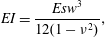 $$\begin{eqnarray}EI=\frac{Esw^{3}}{12(1-\unicode[STIX]{x1D708}^{2})},\end{eqnarray}$$
where
 $I$
is the second moment of area of the panel. Note that the neo-Hookean material model of (2.6) has a nonlinear stress–strain relationship, although it is approximately linear for small deformations (Bonet & Wood Reference Bonet and Wood1997). Here
 $EI$
is set as an input for our material model. Over the following set of simulations, five panel rigidities (see table 1) are selected.
Table of model parameters.

The heaving motion of the panel is actuated with an external force
 $\boldsymbol{G}(\boldsymbol{X},t)$
on the leading edge of the panel. This time-dependent external force may be thought of as arising from stiff tether springs between material points on the panel’s leading edge and virtual points that follow a prescribed motion:
 $$\begin{eqnarray}\boldsymbol{G}(\boldsymbol{X},t)=\left\{\begin{array}{@{}ll@{}}\unicode[STIX]{x1D705}(\unicode[STIX]{x1D74C}_{T}(\boldsymbol{X},t)-\unicode[STIX]{x1D74C}(\boldsymbol{X},t))\quad & \text{if }\boldsymbol{X}\in U_{LE},\\ 0\quad & \text{if }\boldsymbol{X}\notin U_{LE},\end{array}\right.\end{eqnarray}$$
where
 $\unicode[STIX]{x1D705}$
is a spring constant and
 $\unicode[STIX]{x1D74C}_{T}(\boldsymbol{X},t)$
is the desired position of
 $\boldsymbol{X}$
at time
 $t$
. Here
 $U_{LE}\subset U$
represents the portion of the panel where the external force is applied, which is the leading edge of the panel and is 2 % of the panel length. The desired position of the leading edge of tethered panels is
 $$\begin{eqnarray}\unicode[STIX]{x1D74C}_{T}(\boldsymbol{X},t)=\left(\unicode[STIX]{x1D712}_{x}(\boldsymbol{X},0),\unicode[STIX]{x1D712}_{y}(\boldsymbol{X},0),\unicode[STIX]{x1D712}_{z}(\boldsymbol{X},0)+\frac{a}{2}\sin (2\unicode[STIX]{x03C0}\unicode[STIX]{x1D719}t)\right),\end{eqnarray}$$
so that the leading edge is constrained in all three dimensions to move only along the
 $z$
-direction. The untethered panels are unconstrained in the swimming direction, so for this case we modify the first component of
 $\unicode[STIX]{x1D74C}_{T}$
to be
 $\unicode[STIX]{x1D712}_{x}(\boldsymbol{X},t)$
, which effectively eliminates any external force in the
 $x$
-direction. We point out that the elastic forces from the material model are fully three-dimensional. In both the tethered and untethered cases, no background flow is imposed.
2.3 Beam mode analysis
The one-dimensional Euler–Bernoulli beam equation that approximates the deflections
 $H$
of a flexible panel due to an external force is
 $$\begin{eqnarray}\unicode[STIX]{x1D70C}_{p}sw\frac{\unicode[STIX]{x2202}^{2}H}{\unicode[STIX]{x2202}T^{2}}+EI\frac{\unicode[STIX]{x2202}^{4}H}{\unicode[STIX]{x2202}X^{4}}=F_{ext},\end{eqnarray}$$
where
 $\unicode[STIX]{x1D70C}_{p}$
is the density of the panel and
 $F_{ext}$
is the external force per unit length. While the elastohydrodynamic system of the flapping flexible panel in a viscous, incompressible fluid is not fully captured by this equation, its analysis does allow one to identify an important non-dimensional parameter that governs the dynamics and gives insight into the evolving panel kinematics (Paraz et al.
Reference Paraz, Eloy and Schouveiler2014; Quinn et al.
Reference Quinn, Lauder and Smits2014b
, Reference Quinn, Lauder and Smits2015).
Assuming
 $\unicode[STIX]{x1D70C}_{p}/\unicode[STIX]{x1D70C}=O(1)$
and
 $w/s\ll 1$
, the inertia from the panel is dominated by the added mass forces from the fluid, and
 $\unicode[STIX]{x1D70C}_{p}ws$
is replaced by an effective mass per unit length,
 $\unicode[STIX]{x1D70C}sc$
. Defining the dimensionless small parameter
 $\unicode[STIX]{x1D716}^{2}=\unicode[STIX]{x1D70C}_{p}w/\unicode[STIX]{x1D70C}c$
and using the scalings
 $X^{\ast }=X/c,H^{\ast }=H/a,T^{\ast }=T\unicode[STIX]{x1D719}/\unicode[STIX]{x1D716}$
and
 $F_{ext}^{\ast }=(c^{4}/aEI)F_{ext}$
, the beam equation becomes
 $$\begin{eqnarray}\unicode[STIX]{x1D6F1}^{2}\frac{\unicode[STIX]{x2202}^{2}H^{\ast }}{\unicode[STIX]{x2202}T^{\ast 2}}+\frac{\unicode[STIX]{x2202}^{4}H^{\ast }}{\unicode[STIX]{x2202}X^{\ast 4}}=F_{ext}^{\ast },\end{eqnarray}$$
where
 $$\begin{eqnarray}\unicode[STIX]{x1D6F1}=\sqrt{\frac{\unicode[STIX]{x1D70C}sc^{5}\unicode[STIX]{x1D719}^{2}}{EI}}.\end{eqnarray}$$
Here
 $\unicode[STIX]{x1D6F1}$
is a non-dimensional parameter known as the effective flexibility, and
 ${\mathcal{F}}_{ext}^{\ast }\equiv {\mathcal{F}}_{ext}c^{4}/(EIa)$
. The effective flexibility is the ratio of added mass forces from the fluid to the internal bending forces of the elastic panel.
For the boundary conditions
 $H^{\ast }(0,T^{\ast })=0$
and
 $H^{\ast ^{\prime }}(0,T^{\ast })=0$
and
 $H^{\ast ^{\prime \prime }}(1,T^{\ast })=0$
and
 $H^{\ast ^{\prime \prime \prime }}(1,T^{\ast })=0$
one can compute the orthonormal eigenfunctions
 $\unicode[STIX]{x1D6F9}_{i}$
of (2.13) (Weaver, Timoshenko & Young Reference Weaver, Timoshenko and Young1990). This is a natural basis to expand the evolving panel shapes from the computational model. By choosing a cross-section down the middle of the panel and averaging over its thickness, we can describe the panel deflections by
 $H_{sim}^{\ast }(X^{\ast },T^{\ast })$
. For each time
 $T^{\ast }$
, we can write
 $H_{sim}^{\ast }(X^{\ast },T^{\ast })=\sum _{i=1}^{\infty }\unicode[STIX]{x1D6F9}_{i}(X^{\ast })\unicode[STIX]{x1D6E9}_{i}(T^{\ast })$
, where
 $\unicode[STIX]{x1D6F9}_{i}$
are orthonormal eigenfunctions and the
 $\unicode[STIX]{x1D6E9}_{i}$
are their modal contributions. The modal contributions of each eigenfunction are found by taking the inner product of
 $H_{sim}^{\ast }$
with each eigenfunction,
 $$\begin{eqnarray}\unicode[STIX]{x1D6E9}_{i}(T^{\ast })=\int _{0}^{1}H_{sim}^{\ast }(X^{\ast },T^{\ast })\unicode[STIX]{x1D6F9}_{i}(X^{\ast })\,\text{d}X^{\ast }\end{eqnarray}$$
over the length of the panel. Again,
 $H_{sim}^{\ast }$
represents the vertical deflection of the panel resulting from the fluid–structure system. This modal decomposition allows us to separate the deflections of our panel into the sum of the modal contributions of each eigenfunction. At every time step, the panel’s first five modal contributions (
 $\unicode[STIX]{x1D6E9}_{i},i=1,2,3,4,5$
) are recorded.
To understand whether two panels had a similar evolution over the phase of the heaving cycle, we treated the modal contributions of each panel as signals for which we could measure the correlation between pairs. Here the modal contribution correlation of two panels of differing effective flexibilities, panel
 $p$
and panel
 $q$
, is defined as
 $$\begin{eqnarray}\unicode[STIX]{x1D63E}_{i}^{pq}=\frac{1}{N-1}\mathop{\sum }_{n=1}^{N}\frac{\unicode[STIX]{x1D6E9}_{i}^{p}(\unicode[STIX]{x1D709}_{n})-\unicode[STIX]{x1D707}_{i}^{p}}{\unicode[STIX]{x1D70E}_{i}^{p}}\frac{\unicode[STIX]{x1D6E9}_{i}^{q}(\unicode[STIX]{x1D709}_{n})-\unicode[STIX]{x1D707}_{i}^{q}}{\unicode[STIX]{x1D70E}_{i}^{q}},\end{eqnarray}$$
where
 $\unicode[STIX]{x1D6E9}_{i}^{p}$
and
 $\unicode[STIX]{x1D6E9}_{i}^{q}$
are the
 $i$
th modal contributions of panel
 $p$
and panel
 $q$
,
 $\unicode[STIX]{x1D707}_{i}^{p}$
and
 $\unicode[STIX]{x1D70E}_{i}^{p}$
are the mean and standard deviation of
 $\unicode[STIX]{x1D6E9}_{i}^{p}$
,
 $\unicode[STIX]{x1D707}_{i}^{q}$
and
 $\unicode[STIX]{x1D70E}_{i}^{q}$
are the mean and standard deviation of
 $\unicode[STIX]{x1D6E9}_{i}^{q}$
,
 $\unicode[STIX]{x1D709}_{n}$
represents the time points of the phase collected over
 $N$
observations. Here
 $\unicode[STIX]{x1D63E}_{i}^{pq}$
represents the
 $pq$
entry of the correlation matrix,
 $\unicode[STIX]{x1D63E}_{i}\in \mathbb{R}^{120\times 120}$
. Due to differences in the length of the heaving cycle, the modal contributions are interpolated so as to be compared at the same time points of the phase.
Modal contributions do not significantly contribute to the deflection of the panel if their amplitudes are small. Therefore, we weighted the correlations by the mode amplitudes and normalized by the maximum modal contribution of all panels, as follows:
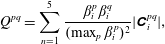 $$\begin{eqnarray}Q^{pq}=\mathop{\sum }_{n=1}^{5}\frac{\unicode[STIX]{x1D6FD}_{i}^{p}\unicode[STIX]{x1D6FD}_{i}^{q}}{(\max _{p}\unicode[STIX]{x1D6FD}_{i}^{p})^{2}}|\unicode[STIX]{x1D63E}_{i}^{pq}|,\end{eqnarray}$$
where
 $$\begin{eqnarray}\unicode[STIX]{x1D6FD}_{i}^{p}=\max _{n}(\unicode[STIX]{x1D6E9}_{i}^{p}(\unicode[STIX]{x1D709}_{n})),\quad \unicode[STIX]{x1D6FD}_{i}^{q}=\max _{n}(\unicode[STIX]{x1D6E9}_{i}^{q}(\unicode[STIX]{x1D709}_{n})).\end{eqnarray}$$
2.4 Circulation analysis
To quantify how the fluid is affected by variations in the effective flexibility, an analysis of the circulation around specific contours was performed. Following the methods of Colin et al. (Reference Colin, Costello, Dabiri, Villanueva, Blottman, Gemmell and Priya2012) and Hoover et al. (Reference Hoover, Griffith and Miller2017), we computed the circulation,
 $\unicode[STIX]{x1D6E4}$
, as the integral of the vorticity component normal to a planar region
 ${\mathcal{R}}$
bounded by a rectangular contour as
 $$\begin{eqnarray}\unicode[STIX]{x1D6E4}=\int _{{\mathcal{R}}}\unicode[STIX]{x1D714}_{y}\,\text{d}x\,\text{d}z,\end{eqnarray}$$
or
 $$\begin{eqnarray}\unicode[STIX]{x1D6E4}=\int _{{\mathcal{R}}}\unicode[STIX]{x1D714}_{z}\,\text{d}x\,\text{d}y,\end{eqnarray}$$
depending on the orientation of interest.
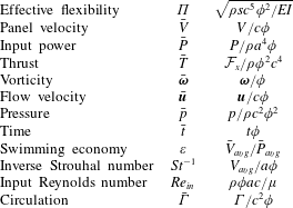
2.5 Non-dimensional parameters
In this study, the panels’ swimming performance is examined using a number of non-dimensional metrics (table 2). Throughout a simulation, the average forward swimming speed
 $V$
of material points of the panel is recorded. This is non-dimensionalized as
 $$\begin{eqnarray}\bar{V}(t)=V(t)/c\unicode[STIX]{x1D719},\end{eqnarray}$$
which corresponds to body lengths per heaving cycle. The total force integrated over the panel,
 ${\mathcal{F}}=({\mathcal{F}}_{x},{\mathcal{F}}_{y},{\mathcal{F}}_{z})$
, is also recorded and we define the non-dimensional thrust as
 $$\begin{eqnarray}\bar{T}(t)={\mathcal{F}}_{x}(t)/(\unicode[STIX]{x1D70C}\unicode[STIX]{x1D719}^{2}c^{4}).\end{eqnarray}$$
Here we choose
 $\unicode[STIX]{x1D719}c$
as a characteristic velocity, due to the absence of a background flow. Non-dimensional input power is also calculated,
 $$\begin{eqnarray}\bar{P}={\mathcal{F}}_{z}V_{LE}/\unicode[STIX]{x1D70C}a^{4}\unicode[STIX]{x1D719},\end{eqnarray}$$
using the heaving amplitude as the characteristic length and
 $V_{LE}$
as the leading edge velocity. The Eulerian variables have non-dimensional analogues for flow velocity (
 $\bar{\boldsymbol{u}}=\boldsymbol{u}/c\unicode[STIX]{x1D719}$
), vorticity (
 $\bar{\unicode[STIX]{x1D74E}}=\unicode[STIX]{x1D74E}/\unicode[STIX]{x1D719}$
) and pressure (
 $\bar{p}=p/\unicode[STIX]{x1D70C}c^{2}\unicode[STIX]{x1D719}^{2}$
). Time is non-dimensionalized with respect to the heaving frequency (
 $\bar{t}=t\unicode[STIX]{x1D719}$
). The circulation,
 $\unicode[STIX]{x1D6E4}$
, is non-dimensionalized with respect to the chord length,
 $c$
, and heaving frequency,
 $\unicode[STIX]{x1D719}$
,
 $$\begin{eqnarray}\bar{\unicode[STIX]{x1D6E4}}=\frac{\unicode[STIX]{x1D6E4}}{c^{2}\unicode[STIX]{x1D719}}.\end{eqnarray}$$
See table 2.
Table of non-dimensional parameters.
Other metrics are used to quantify a panel’s performance. The swimming economy, which is the energy cost per unit of distance travelled, is defined here as
 $$\begin{eqnarray}\unicode[STIX]{x1D700}=\bar{V}_{avg}/\bar{P}_{avg},\end{eqnarray}$$
where
 $\bar{V}_{avg}$
and
 $\bar{P}_{avg}$
are, respectively, the non-dimensional speed and input power averaged over the duration of a panel’s heaving cycle. We also consider the Strouhal number,
 $$\begin{eqnarray}St=\frac{a\unicode[STIX]{x1D719}}{V_{avg}}\end{eqnarray}$$
as another performance metric. Swimming and flying animals have been characterized as achieving peak propulsive efficiencies for
 $0.2<St<0.4$
(Taylor, Nudds & Thomas Reference Taylor, Nudds and Thomas2003).
The Reynolds number is a non-dimensional parameter that characterizes the ratio of inertial force to viscous forces. In this study, we report the Reynolds number using a frequency-based definition,
 $$\begin{eqnarray}Re_{in}=\frac{\unicode[STIX]{x1D70C}a\unicode[STIX]{x1D719}c}{\unicode[STIX]{x1D707}},\end{eqnarray}$$
where
 $a\unicode[STIX]{x1D719}$
is the characteristic velocity. Note that we use a frequency-based characteristic velocity rather than the resulting swimming speed so that
 $Re_{in}$
is an input value known at the start of a simulation. In this simulations presented in this study, the maximum value of
 $Re_{in}$
is 750. Alternatively, using the resulting average swimming speed of an untethered panel as a characteristic velocity would yield Reynolds numbers that are at most 1500.
2.6 Computational implementation
The numerical model was implemented using IBAMR, which is a distributed-memory parallel implementation of the IB method that includes Cartesian grid adaptive mesh refinement (AMR) (IBAMR 2014). IBAMR relies on several open-source libraries, including SAMRAI (Hornung, Wissink & Kohn Reference Hornung, Wissink and Kohn2006; SAMRAI 2007), PETSc (Balay et al. Reference Balay, Gropp, McInnes, Smith and Arge1997, Reference Balay, Abhyankar, Adams, Brown, Brune, Buschelman, Eijkhout, Gropp, Kaushik and Knepley2009), hypre (Falgout & Yang Reference Falgout, Yang and Sloot2002; HYPRE 2011) and libMesh (Kirk et al. Reference Kirk, Peterson, Stogner and Carey2006).
The computational domain was taken to be a rectangular box of length
 $8c\times 4c\times 4c$
with periodic boundary conditions in the axial direction and no-slip boundary conditions otherwise. The domain was discretized using an adaptively refined grid for which the finest Cartesian grid domain discretization would result in a
 $1024\times 512\times 512$
patch (figure 1), where the finest spatial grid size is
 $h=4c/512$
. The time step was taken to be
 $\unicode[STIX]{x0394}t=1\times 10^{-4}~\text{s}$
and
 $5\times 10^{-5}~\text{s}$
, where the latter, more refined step size was used for panels with bending moduli of
 $1\times 10^{-6}$
and
 $5\times 10^{-7}~\text{N}~\text{m}^{2}$
. Comparing the simulations with domain discretizations of
 $512\times 256\times 256$
,
 $2048\times 1024\times 1024$
and
 $4096\times 2048\times 2048$
patches, we found better than linear convergence of the resulting panel swimming speed (
 $O(h^{1.3})$
). Further convergence studies of the IBAMR method and framework can be found in Griffith & Luo (Reference Griffith and Luo2016) and Tytell et al. (Reference Tytell, Leftwich, Hsu, Griffith, Cohen, Smits, Hamlet and Fauci2016). We note that for all simulations the computational domain has been chosen large enough so that there is no discernible interaction between the panel and the boundaries of the computational domain.
Plot displaying the domain discretization using adaptive mesh refinement from IBAMR, where the most refined discretization is reserved for portions of the domain where the structure is present and the vorticity magnitude is above a certain threshold, here plotted for
 $|\bar{\unicode[STIX]{x1D74E}}|>4$
.

3 Results
In this study, model panels with varying rigidity (see table 1) were heaved sinusoidally at an amplitude of
 $a=0.1c$
, with heaving frequencies that ranged from 0.125 to
 $3.0~\text{s}^{-1}$
in 0.125
 $\text{s}^{-1}$
increments. The panel begins at rest in a domain of quiescent flow and is then heaved with the body force described in (2.10) and (2.11).
Plots of (a) dimensionless swimming speed (
 $\bar{V}$
) and (b) input power (
 $\bar{P}$
) for an untethered panel with a bending modulus of
 $EI=1\times 10^{-7}~\text{N}~\text{m}^{2}$
being heaved sinusoidally with a frequency of
 $\unicode[STIX]{x1D719}=0.5~\text{s}^{-1}$
. Here
 $Re_{in}=125$
. Note that the panel stabilizes after the third cycle.
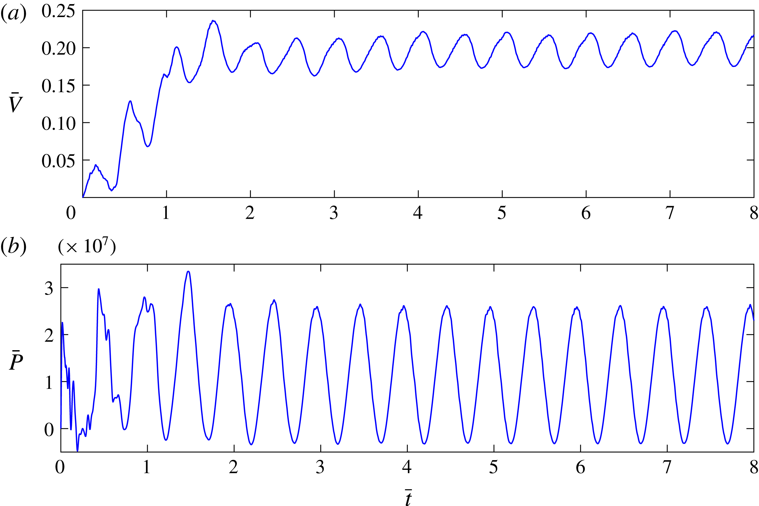
Figure 2 shows the time evolution of non-dimensional panel speed (
 $\bar{V}$
) and input power (
 $\bar{P}$
) as a function of heaving cycles for a representative panel (
 $EI=1\times 10^{-7}~\text{N}~\text{m}^{2}$
,
 $\unicode[STIX]{x1D719}=0.5~\text{s}^{-1}$
). After approximately two heaving cycles the velocity of the panel reaches a steady periodic state. Input power also reaches a steady-state cycle (figure 2
b).
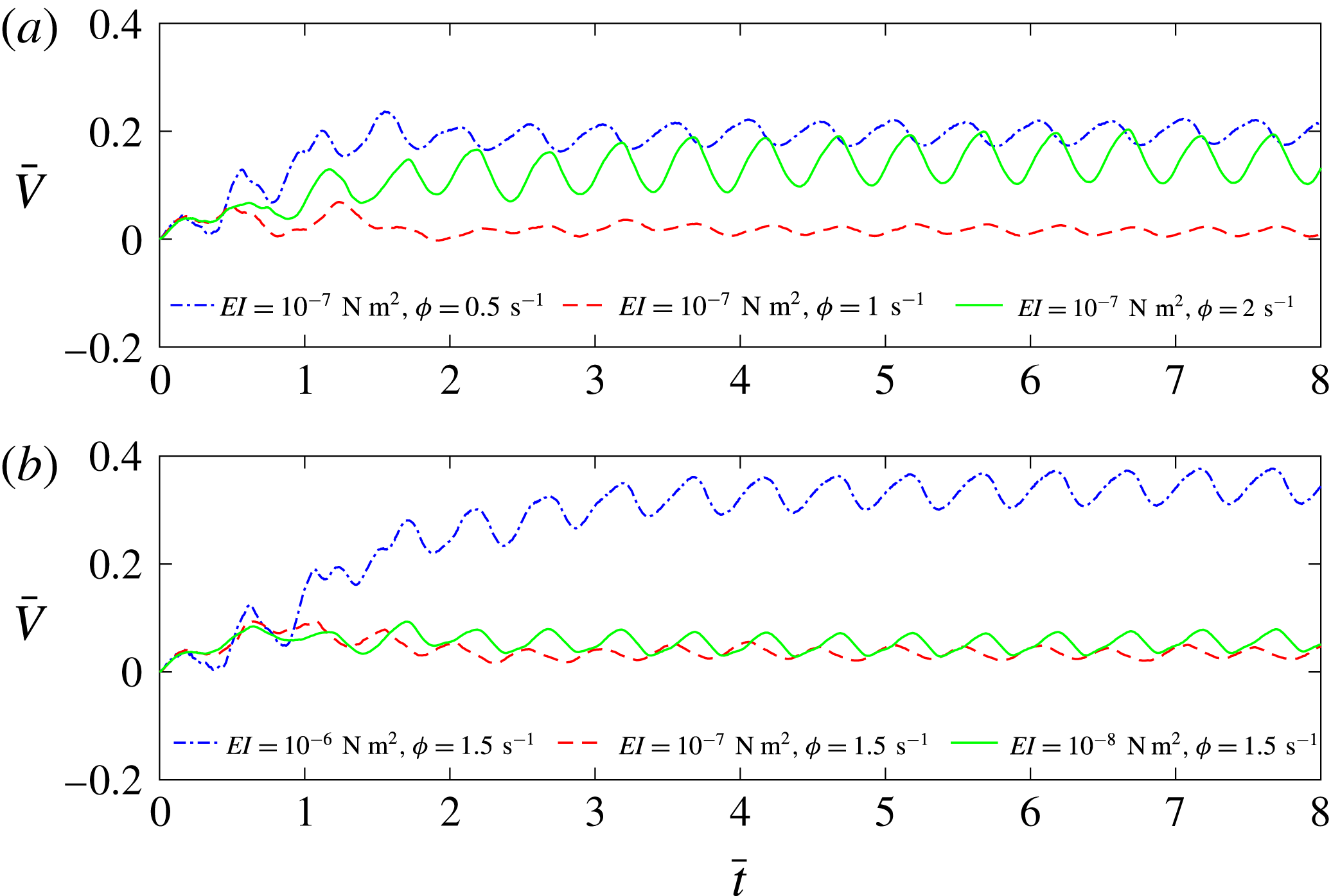
We also compared the cycle-to-cycle swimming performance of panels with different bending moduli or actuated at different frequencies (figure 3). In all of the simulations, the panel quickly reaches a steady-state behaviour following the initial heaving cycles, where cycle-to-cycle variations of the swimming speed are minimal. In figure 3(a) the swimming speed is plotted as a function of cycle number for the same panel actuated at different frequencies. Note that the swimming speed of this panel does not increase monotonically as frequency increases. This is because the resulting waveform of the panel is different for different heaving frequencies. This will be more closely examined below. In figure 3(b), swimming speed is plotted for three different panels of varying bending moduli that were actuated at the same frequency. There is not a monotonic change in swimming speed with respect to bending modulus. Clearly there is an interplay between the elastic properties of the panel and the fluid forces that it experiences at different frequencies. In the following sections, we analyse the swimming performance as a function of the effective flexibility
 $\unicode[STIX]{x1D6F1}$
of the heaving panel, which is the non-dimensional parameter that characterizes this interplay.
Comparison plots of the dimensionless swimming speed (
 $\bar{V}$
) as a function of the cycle for three panels where (a) the bending modulus (
 $EI$
) is fixed and the heaving frequency (
 $\unicode[STIX]{x1D719}$
) is varied, and (b) the heaving frequency is fixed and the bending modulus is varied.
Plots of (a) trailing edge amplitude, (b) forward swimming speed (
 $V_{avg}$
) and (c) dimensionless forward swimming speed (
 $\bar{V}_{avg}$
) as a function of the effective flexibility (
 $\unicode[STIX]{x1D6F1}$
) of a panel. Here the different coloured lines represent the differing bending moduli (
 $EI$
) of the panels. The range of effective flexibility values were spanned by varying the heaving frequency (
 $\unicode[STIX]{x1D719}$
) of a panel from 0.125
 $\text{s}^{-1}$
to 3.0
 $\text{s}^{-1}$
.

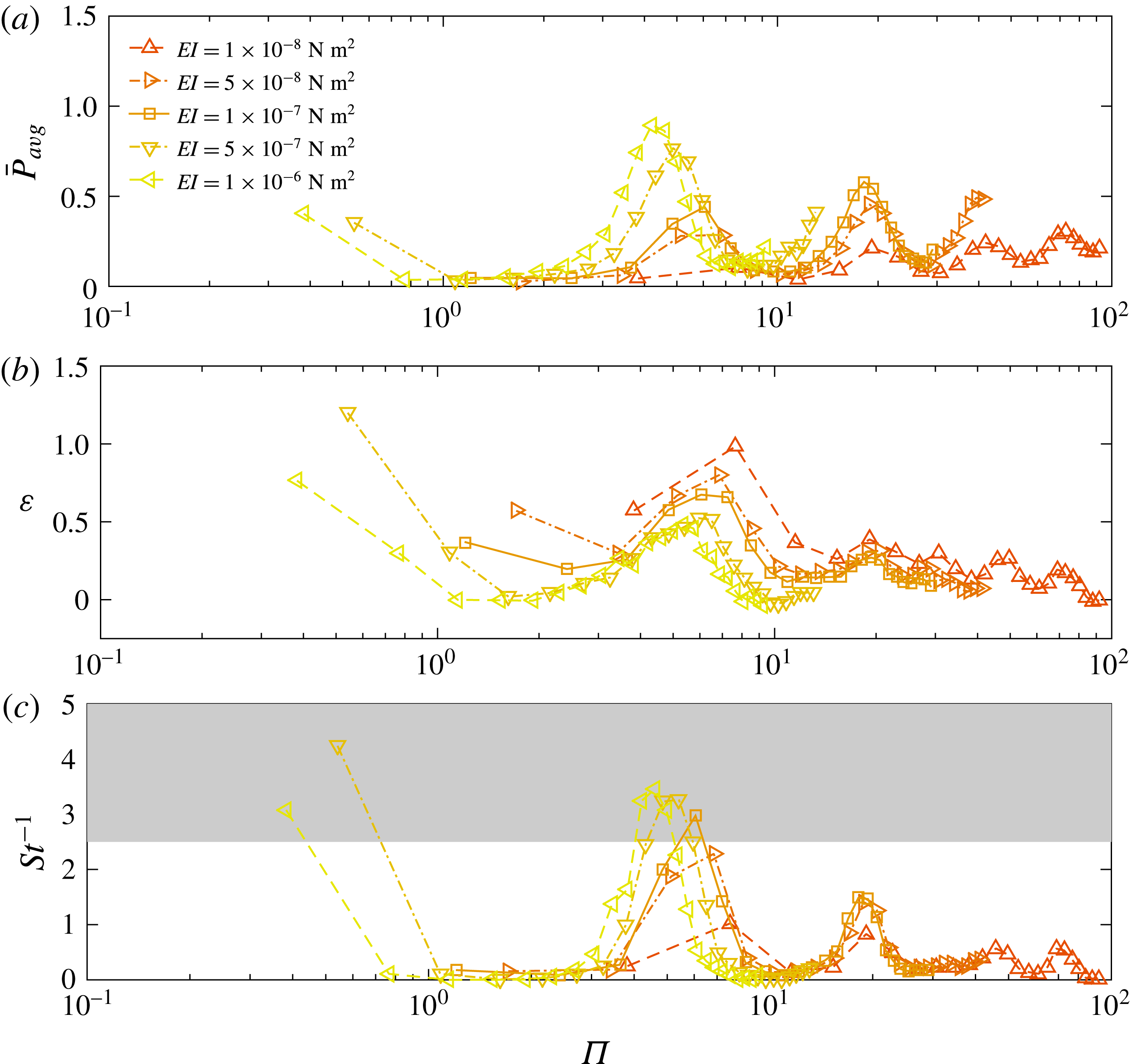
Plots of the panels’ (a) average power consumption (
 $\bar{P}_{avg}$
), (b) swimming economy (
 $\unicode[STIX]{x1D700}$
), and (c) inverse Strouhal number (
 $St^{-1}$
) as a function of the effective flexibility (
 $\unicode[STIX]{x1D6F1}$
) of the panels. We find that for fixed
 $\unicode[STIX]{x1D6F1}$
value, the more flexible panel has a higher swimming economy. The inverse Strouhal number reveals that the two stiffest panels actuated at effective flexibilities near the first two resonant peaks correspond to the range of Strouhal numbers (in grey) associated with high efficiency swimming and flying (Taylor et al.
Reference Taylor, Nudds and Thomas2003).
3.1 Propulsive performance
We performed computational experiments on five panels that differed in bending moduli and were actuated at a range of frequencies. In each of these simulations, the shape of the untethered panel and its swimming progression emerge from the full coupled system. For each of the five panels, figure 4(a) shows the normalized trailing edge amplitude achieved by the panel as a function of the effective flexibility as it is actuated at different frequencies. We see that peaks in trailing edge amplitude occur near certain effective flexibilities, and these basically coincide for each of the panels. Moreover, the trailing edge amplitude varied little for panels actuated with similar effective flexibilities even when their bending moduli differed. Following the classic definition (Den Hartog Reference Den Hartog1985) and more recently that by Quinn et al. (Reference Quinn, Lauder and Smits2014b
), we refer to the system as operating in resonance when the trailing edge amplitude reaches a local maximum at certain values of the effective flexibility
 $\unicode[STIX]{x1D6F1}$
(or, equivalently, the oscillation frequency
 $\unicode[STIX]{x1D719}$
). Figure 4(a) shows that there are at least four such resonant peaks in the range of effective flexibilities that we studied.
The peaks in trailing edge amplitude correspond to peaks in average swimming speed. Figure 4(b) shows the average (dimensional) swimming speed
 $V_{avg}$
as a function of effective flexibility. Although the peaks in
 $V_{avg}$
and trailing edge amplitude occur at similar effective flexibilities, the resulting swimming speeds depend on the bending moduli of the panel. Stiffer panels had higher
 $V_{avg}$
compared to the more flexible panels heaved at similar effective flexibilities. Of course, different material panels must be actuated at different frequencies in order to achieve the same effective flexibility. Figure 4(c) shows the swimming speed divided by
 $c\unicode[STIX]{x1D719}$
, which corresponds to body lengths per heaving cycle (
 $\bar{V}_{avg}$
). We see that this non-dimensional velocity is better matched for panels actuated at similar effective flexibilities, but the most flexible panels still move more slowly.
In figure 5(a), we plot the average input power
 $\bar{P}_{avg}$
, and we note that local peaks of input power coincide with local peaks in velocity (figure 4
b) – the highest swimming speeds require the most power input. Figure 5(b) plots the swimming economy as a function of effective flexibility. While the peaks of average velocity and power occur at the same value of effective flexibility, the swimming economy, which is the ratio of these values, need not achieve a local maximum there. In fact, we find that the peak in economy occurs at slightly higher values of
 $\unicode[STIX]{x1D6F1}$
because the amplitude tapers off more slowly than power as
 $\unicode[STIX]{x1D6F1}$
increases. Similar shifts in efficiency peaks were noted in the model of Michelin & Llewellyn Smith (Reference Michelin and Llewellyn Smith2009). We also see that input power is higher for stiffer panels than more flexible panels near the same effective flexibility. This in turn leads stiffer panels to have peaks in swimming economy at lower effective flexibilities than more flexible panels and to have a lower swimming economy overall compared to more flexible panels, even at the same effective flexibility. Note that to achieve a fixed effective flexibility, a stiff panel must be heaved at a higher frequency than a more flexible panel. This would increase the power required to complete the heaving motion. However, stiffer panels have a higher inverse Strouhal number than more flexible ones figure 5(c). While each tailbeat results in greater forward motion when compared to the tailbeat of a more flexible panel, more energy is expended for the motion. We plot inverse Strouhal numbers rather than Strouhal numbers, because at very low swimming speeds, the Strouhal number approaches infinity. The stiffest panels actuated so that their effective flexibilities are near the first two resonant peaks reach Strouhal numbers in the range associated with peak propulsive efficiency,
 $0.2<St<0.4$
(Taylor et al.
Reference Taylor, Nudds and Thomas2003).
3.2 Modal contributions
By choosing a cross-section down the middle of the panel and averaging over its thickness, we can represent its emergent, time-periodic oscillations by a one-dimensional curve. This curve can be decomposed into the eigenfunctions of the beam equation as discussed in § 2.3. For each simulation, the first five modal contributions of the heaving panel (
 $\unicode[STIX]{x1D6E9}_{i}(t)$
,
 $i=1,2,3,4,5$
) were calculated at every time step. Figure 6(a) shows the time-dependent modal contributions of a representative panel simulation (
 $EI=1\times 10^{-7}~\text{N}~\text{m}^{2}$
,
 $\unicode[STIX]{x1D719}=0.5~\text{s}^{-1}$
) as it moves through eight heaving cycles. Each
 $\unicode[STIX]{x1D6E9}_{i}$
represents the weight of the eigenfunction,
 $\unicode[STIX]{x1D6F9}_{i}$
, with respect to the deflection of the panel. Following the initial heaving cycles, all of the panel’s modal contributions tend toward steady cycles. Although each of the modal contributions have the same frequency as the heaving frequency, they differ in both amplitude and phase.
(a) Plot of the modal contribution of the first five modes with respect to the heaving cycles of a panel (
 $EI=1\times 10^{-7}~\text{N}~\text{m}^{2}$
,
 $\unicode[STIX]{x1D719}=0.5~\text{s}^{-1}$
). Starting from rest initially, the modal contributions of the panel deflection quickly follow a sinusoidal pattern, with each modal contribution varying in amplitude and peak point in the phase. (b) Plots of the modal contributions of the first (red) and second (magenta) mode for three different panels. (c) Plot of the maximum modal contribution of each mode with respect to the heaving panels’ effective flexibility. Higher mode contributions increase as effective flexibility increases.
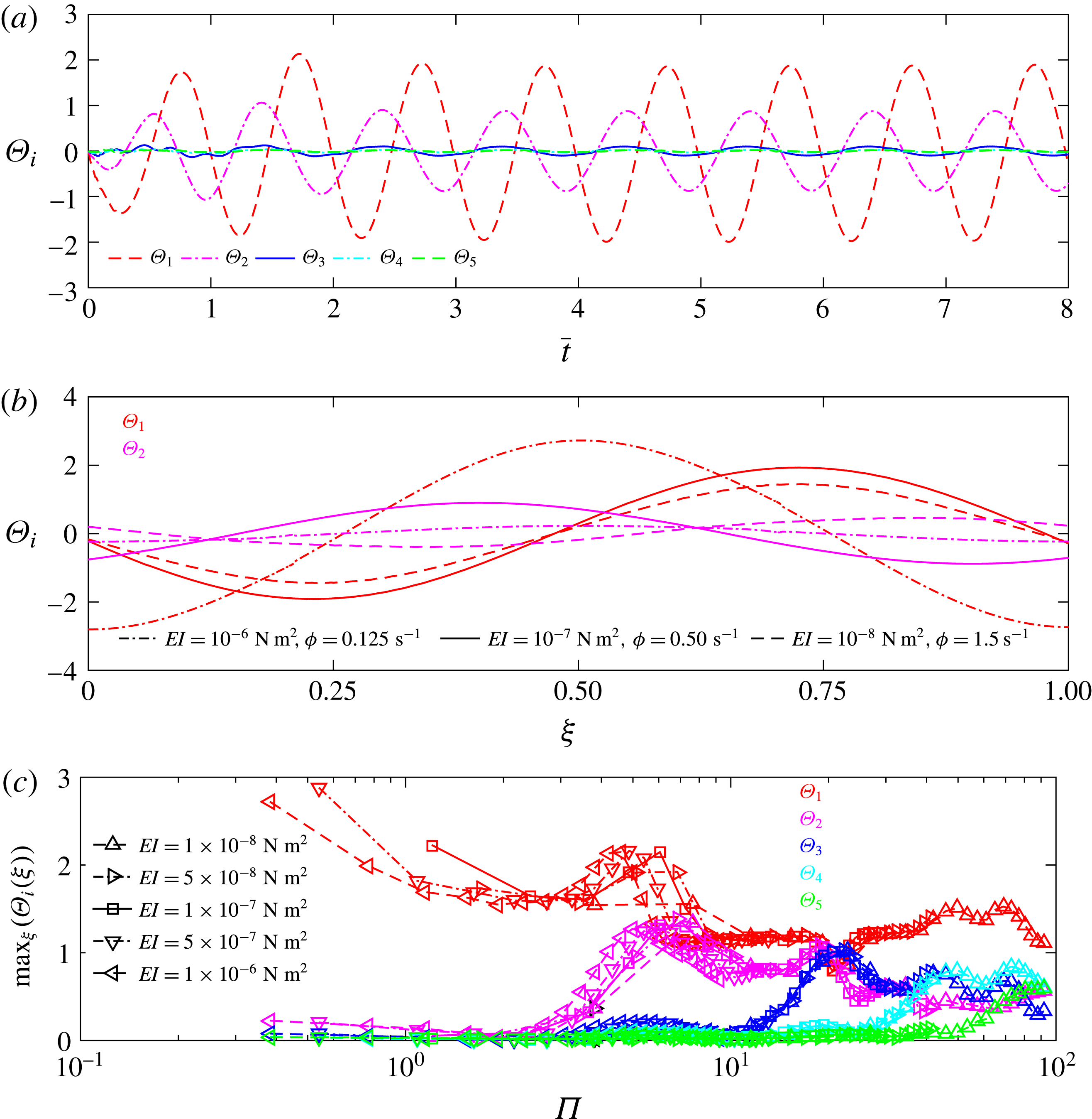
The amplitude and phase of each mode depends on the effective flexibility. Figure 6(b) shows the shape of the panel when approximated only by the contribution of the first mode,
 $\unicode[STIX]{x1D6E9}_{1}$
(in red), over the phase
 $\unicode[STIX]{x1D709}\in [0,1)$
, for three panels of differing effective flexibilities (
 $EI=1\times 10^{-6}~\text{N}~\text{m}^{2}$
,
 $\unicode[STIX]{x1D719}=0.125~\text{s}^{-1}$
;
 $\unicode[STIX]{x1D6F1}=0.3827$
,
 $EI=1\times 10^{-7}~\text{N}~\text{m}^{2}$
,
 $\unicode[STIX]{x1D719}=0.5~\text{s}^{-1}$
;
 $\unicode[STIX]{x1D6F1}=4.8412$
and
 $EI=1\times 10^{-8}~\text{N}~\text{m}^{2}$
,
 $\unicode[STIX]{x1D719}=1.5~\text{s}^{-1}$
;
 $\unicode[STIX]{x1D6F1}=45.9279$
). For the two most flexible panels,
 $\unicode[STIX]{x1D6E9}_{1}$
has a similar amplitude and phase, while that for the third one is shifted and has a larger amplitude. Figure 6(b) also shows the contribution of the second mode to the panel’s shape,
 $\unicode[STIX]{x1D6E9}_{2}$
(in magenta). We see that the similarities between the more flexible panels are absent in the second mode, with significant differences in amplitude and phase in
 $\unicode[STIX]{x1D6E9}_{2}$
for all three panels.
As the effective flexibility increases, each of the higher-order modes emerge sequentially, and each new mode contributes to a resonant peak in amplitude and performance. Figure 6(c) shows the maximum contribution of each mode,
 $\max _{\unicode[STIX]{x1D709}}(\unicode[STIX]{x1D6E9}_{i}(\unicode[STIX]{x1D709}))$
, for all panels. At lower effective flexibilities, the modal contribution from the first mode dominates, indicating that the higher modes contribute little to the shape of the panel. As effective flexibility increases, the modal contributions of higher modes emerge sequentially. Their emergence is followed by a peak in the maximum modal contribution of that mode. The effective flexibilities at which a peak modal contribution occurs coincide with the effective flexibilities where peak trailing edge amplitudes and velocities occur (compare to figure 4).
3.3 Phase evolution
Not only are the amplitudes of the modal contributions similar when the effective flexibility is the same, but the evolution of the mode over the cycle is also similar. In figure 6(b), the maximum modal contributions of the first mode of two panels (
 $EI=1\times 10^{-7}~\text{N}~\text{m}^{2}$
,
 $\unicode[STIX]{x1D719}=0.5~\text{s}^{-1}$
and
 $EI=1\times 10^{-8}~\text{N}~\text{m}^{2}$
,
 $\unicode[STIX]{x1D719}=1.5~\text{s}^{-1}$
) occurred at similar phase, while the maximum modal contributions for the third panel (
 $EI=1\times 10^{-6}~\text{N}~\text{m}^{2}$
,
 $\unicode[STIX]{x1D719}=0.125~\text{s}^{-1}$
) occurs at a different phase. To quantify the similarity or difference in the evolution of the mode shapes for different panels, we used (2.17) to compute a normalized correlation
 $Q^{pq}$
between panels
 $p$
and
 $q$
. This value is high when the phase evolution of the
 $i$
th mode is correlated in the phase between the two panels and has a large amplitude.
 $Q$
value from (2.17) associated with two panels, ordered by the two panels’ effective flexibility. Note that higher
 $Q$
values indicated that the modes of two panels are correlated and that the amplitude of modal contributions associated with both panels are substantial.

Figure 7 shows the value of
 $Q$
for all pairs of heaving panels arranged by effective flexibility. The high
 $Q$
values along the diagonal show that panels with good swimming performance and high amplitude modal contributions have a similar shape evolution over the phase as panels with similar effective flexibilities. These correspond to the peaks in trailing edge amplitude (figure 4
a) and swimming speed (figure 4
c). This suggests that panels with high
 $\bar{V}_{avg}$
and similar
 $\unicode[STIX]{x1D6F1}$
also have similar shape evolutions over the phase of the heaving cycle. The exact locations of the resonant peaks vary slightly as a function of the panel’s bending rigidity, accounting for relatively high
 $Q$
values off the diagonal at
 $\unicode[STIX]{x1D6F1}\approx 8$
.
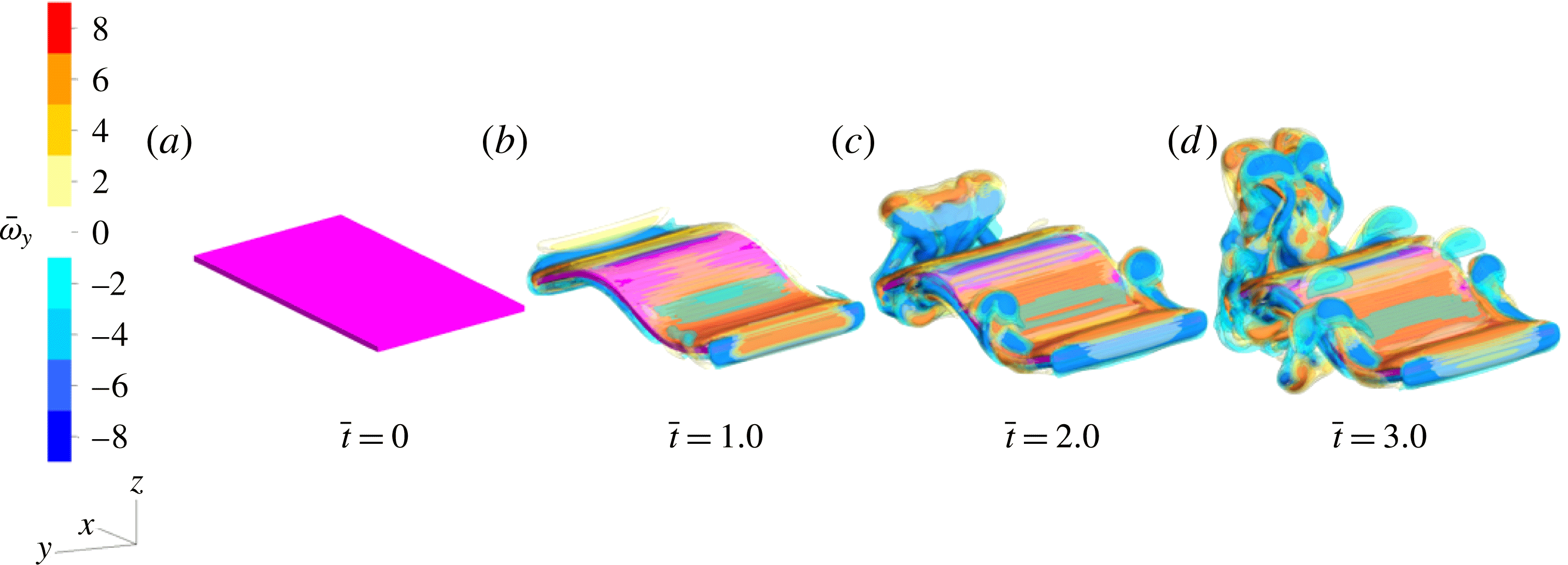
Isocontour plots of the dimensionless
 $y$
-component of vorticity,
 $\bar{\unicode[STIX]{x1D714}}_{y}$
, at the start of the first through fourth heaving cycles (from left to right). The panel is of
 $\unicode[STIX]{x1D6F1}=19.3649$
(
 $EI=1\times 10^{-7}~\text{N}~\text{m}^{2}$
,
 $\unicode[STIX]{x1D719}=2.0~\text{s}^{-1}$
) and
 $Re_{in}=500$
. Note that after the first heaving cycle, the deflection of the panel is nearly identical at the start of each heaving cycle, although the resulting vorticity field varies in time.
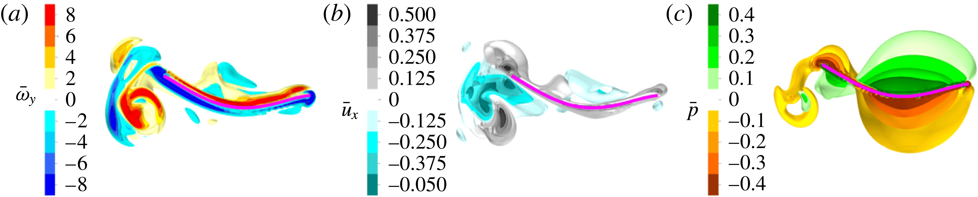
Isocontour plots, cut out along the centre plane, of the (a) dimensionless
 $y$
-component of vorticity (
 $\bar{\unicode[STIX]{x1D714}}_{y}$
), (b) dimensionless
 $x$
-component of flow velocity (
 $\bar{u}_{x}$
) and (c) dimensionless pressure (
 $\bar{p}$
) during the start of the third heaving cycle of a panel with
 $\unicode[STIX]{x1D6F1}=6.0515$
(
 $EI=1\times 10^{-7}~\text{N}~\text{m}^{2}$
,
 $\unicode[STIX]{x1D719}=0.625~\text{s}^{-1}$
).
3.4 Flow patterns
The fluid flow resulting from the panels’ heaving motion is examined via dimensionless vorticity,
 $\bar{\unicode[STIX]{x1D74E}}$
. Figure 8 shows an example of the development of the flow in the first four heaving cycles. Although the vortex structures present in the wake grow after each heaving cycle, the shape of the panel at the start of the cycle and the vortex structures in the immediate wake remain fairly constant following the initial heaving cycle.
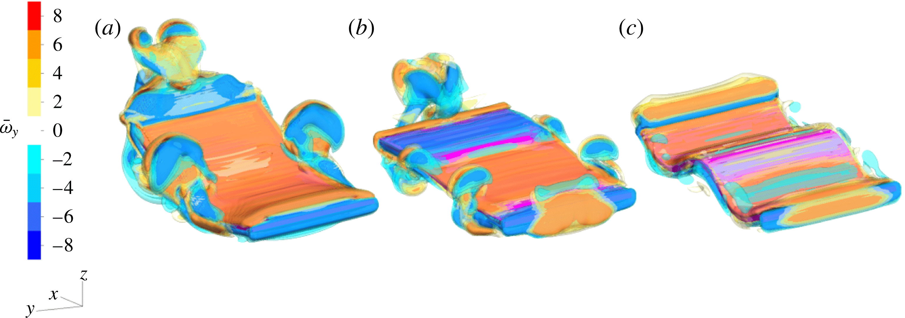
Isocontour plots of the dimensionless
 $y$
-component of vorticity,
 $\bar{\unicode[STIX]{x1D714}}_{y}$
, at the start of the third heaving cycle for three panels heaved at the same frequency,
 $\unicode[STIX]{x1D719}=1.5~\text{s}^{-1}$
, but with
 $EI$
equal to (a)
 $1\times 10^{-6}~\text{N}~\text{m}^{2}$
(
 $\unicode[STIX]{x1D6F1}=4.5928$
), (b)
 $1\times 10^{-7}~\text{N}~\text{m}^{2}$
(
 $\unicode[STIX]{x1D6F1}=14.5237$
), (c)
 $1\times 10^{-8}~\text{N}~\text{m}^{2}$
(
 $\unicode[STIX]{x1D6F1}=45.9279$
).
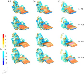
Isocontour plots of the dimensionless
 $y$
-component of vorticity,
 $\bar{\unicode[STIX]{x1D714}}_{y}$
, during the heaving cycle for three panels of similar effective flexibility, with
 $\unicode[STIX]{x1D6F1}$
equal to (a)
 $5.7410$
(
 $EI=1\times 10^{-6}~\text{N}~\text{m}^{2}$
,
 $\unicode[STIX]{x1D719}=1.625~\text{s}^{-1}$
,
 $Re_{in}=406.25$
), (b)
 $5.4127$
(
 $EI=5\times 10^{-7}~\text{N}~\text{m}^{2}$
,
 $\unicode[STIX]{x1D719}=1.250~\text{s}^{-1}$
,
 $Re_{in}=312.5$
), (c)
 $6.0515$
(
 $EI=1\times 10^{-7}~\text{N}~\text{m}^{2}$
,
 $\unicode[STIX]{x1D719}=0.625~\text{s}^{-1}$
,
 $Re_{in}=156.25$
). Snapshots are taken at
 $\bar{t}$
(from top to down) 3.0, 3.25, 3.50 and 3.75.
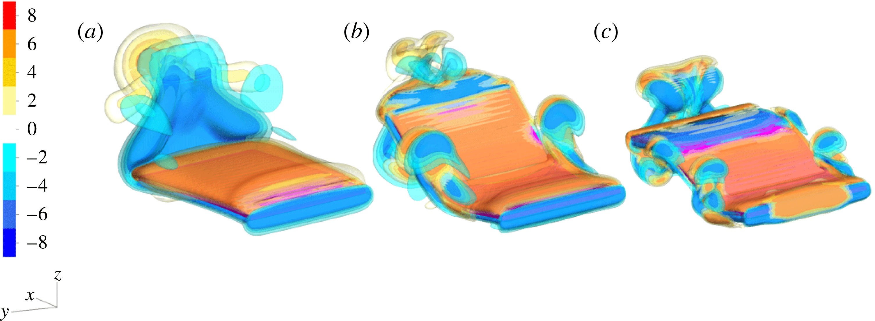
Isocontour plots of the dimensionless
 $y$
-component of vorticity,
 $\bar{\unicode[STIX]{x1D714}}_{y}$
, at the start of the third heaving cycle for three panels that swim rapidly but have different effective flexibilities,
 $\unicode[STIX]{x1D6F1}$
equal to (a)
 $0.5413$
(
 $EI=5\times 10^{-7}~\text{N}~\text{m}^{2}$
,
 $\unicode[STIX]{x1D719}=0.125~\text{s}^{-1}$
,
 $Re_{in}=31.25$
), (b)
 $6.0515$
(
 $EI=1\times 10^{-7}~\text{N}~\text{m}^{2}$
,
 $\unicode[STIX]{x1D719}=0.625~\text{s}^{-1}$
,
 $Re_{in}=156.25$
), (c)
 $17.116$
(
 $EI=5\times 10^{-8}~\text{N}~\text{m}^{2}$
,
 $\unicode[STIX]{x1D719}=1.250~\text{s}^{-1}$
,
 $Re_{in}=312.5$
).
Plots of the dimensionless
 $y$
-component of vorticity along the central plane at the end of the fourth heaving cycle for panels with
 $\unicode[STIX]{x1D6F1}$
equal to (a) 0.5143 (
 $EI=5\times 10^{-7}~\text{N}~\text{m}^{2}$
,
 $\unicode[STIX]{x1D719}=0.125~\text{s}^{-1}$
), (b) 6.0515 (
 $EI=1\times 10^{-7}~\text{N}~\text{m}^{2}$
,
 $\unicode[STIX]{x1D719}=0.625~\text{s}^{-1}$
) and (c) 17.116 (
 $EI=5\times 10^{-8}~\text{N}~\text{m}^{2}$
,
 $\unicode[STIX]{x1D719}=1.25~\text{s}^{-1}$
). The three panels are representative of the panels with
 $\unicode[STIX]{x1D6F1}$
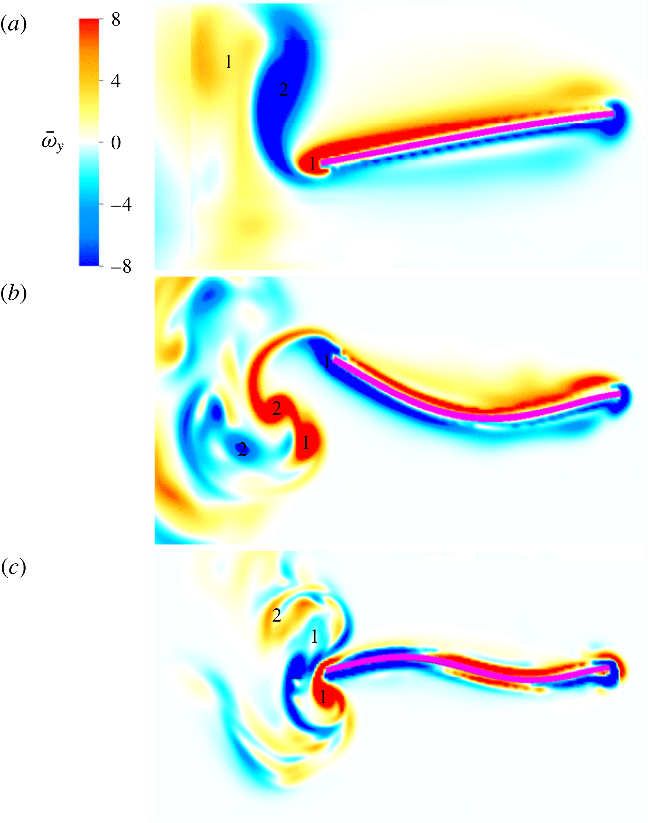
values associated with the first three resonant peaks. In (a) we note the presence of a 2S vortex shedding pattern, while in (b,c) the 2P vortex shedding pattern is present.
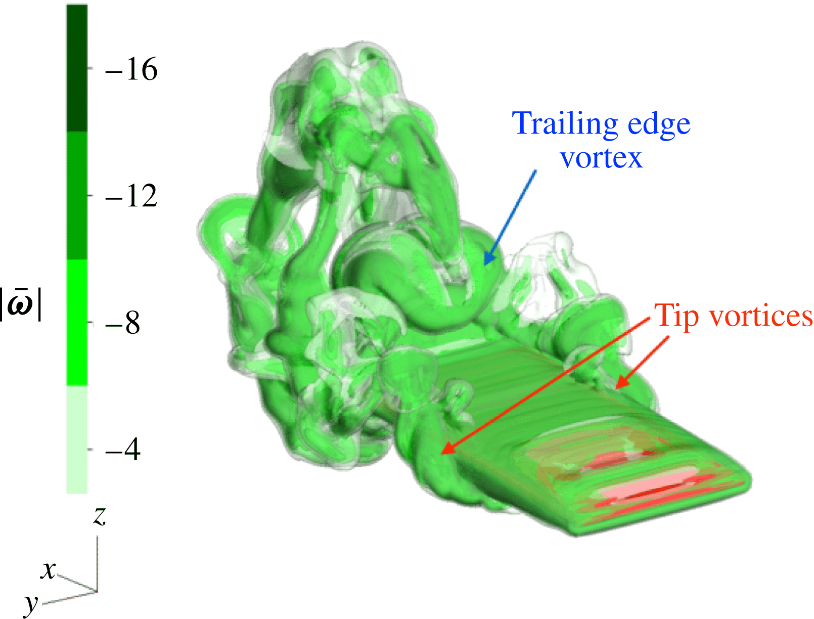
Plot of the dimensionless vorticity magnitude,
 $|\bar{\unicode[STIX]{x1D74E}}|$
, near the point of peak panel swimming speed for a panel with
 $\unicode[STIX]{x1D6F1}=5.7410$
(
 $EI=1\times 10^{-6}~\text{N}~\text{m}^{2}$
,
 $\unicode[STIX]{x1D719}=1.625~\text{s}^{-1}$
,
 $Re_{in}=312.5$
). The tip vortices and trailing edge vortex are highlighted.
Isocontour plots of the dimensionless
 $z$
-component of vorticity,
 $\bar{\unicode[STIX]{x1D714}}_{z}$
, near the point of peak panel swimming speed during the heaving cycle for three panels with similar effective flexibilities,
 $\unicode[STIX]{x1D6F1}$
equal to (a)
 $5.7410$
(
 $EI=1\times 10^{-6}~\text{N}~\text{m}^{2}$
,
 $\unicode[STIX]{x1D719}=1.625~\text{s}^{-1}$
,
 $Re_{in}=406.25$
), (b)
 $5.4127$
(
 $EI=5\times 10^{-7}~\text{N}~\text{m}^{2}$
,
 $\unicode[STIX]{x1D719}=1.25~\text{s}^{-1}$
,
 $Re_{in}=312.5$
), (c)
 $6.0515$
(
 $EI=1\times 10^{-7}~\text{N}~\text{m}^{2}$
,
 $\unicode[STIX]{x1D719}=0.625~\text{s}^{-1}$
,
 $Re_{in}=156.25$
).

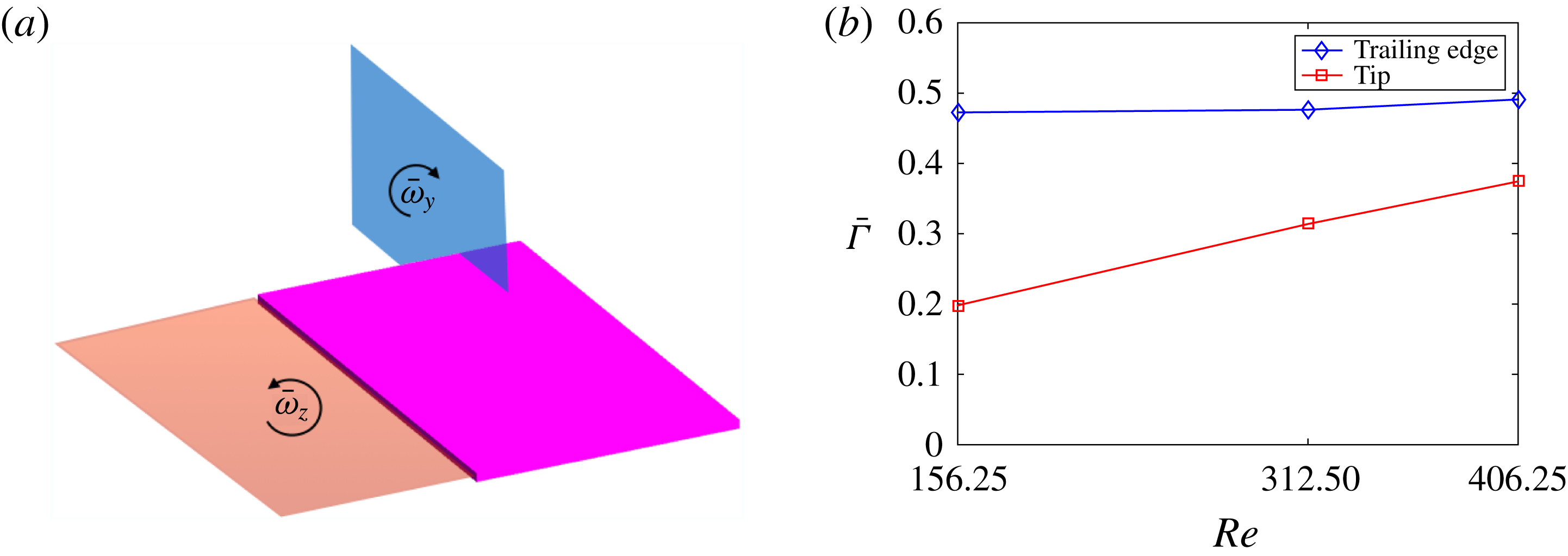
(a) Diagram of the planes from which the circulation of the trailing vortex (blue) and the tip vortices (red) were calculated. (b) Plot of the circulation,
 $\bar{\unicode[STIX]{x1D6E4}}$
, of the trailing edge vortices (blue) and the tip vortices (red) for the panels of figures 11 and 15 as a function of
 $Re$
.
In figure 9, we compare the isocontours along the centre plane for the spanwise (
 $y$
) vorticity (
 $\bar{\unicode[STIX]{x1D714}}_{y}$
), axial (
 $x$
) velocity (
 $\bar{u}_{x}$
) and pressure (
 $\bar{p}$
) at the start of the third heaving cycle for a panel with a substantial swimming speed (
 $EI=1\times 10^{-7}~\text{N}~\text{m}^{2}$
,
 $\unicode[STIX]{x1D719}=0.625~\text{s}^{-1}$
). The trailing edge generates alternating vortex structures (figure 9
a). These vortices then generate a region of positive axial flow (
 $\bar{u}_{x}$
) near the trailing edge of the panel (grey region in figure 9
b). This zone of positive axial velocity corresponds to the presence of positive pressure near the trailing edge of the panel and negative pressure on the opposite side (figure 9
c), which combine to give the thrust force. We also find zones of positive and negative pressure on opposite sides of the panel due to the deflections of the panel.
Differences in the panel shape evolution yield differences in the resulting flow structures. Figure 10 compares the
 $\bar{\unicode[STIX]{x1D714}}_{y}$
isocontours at the start of the third heaving cycle for three panels, with differing passive material properties and identical heaving frequencies. The differences in the observed flow structures in turn account for differences in panel performance. Similar observations can be made when examining
 $\bar{\unicode[STIX]{x1D714}}_{y}$
isocontours of three panels with identical passive material properties but differing heaving frequencies. Movies of both comparisons can be found in the supplementary material available at https://doi.org/10.1017/jfm.2018.305.
Above we have shown that panels with similar effective flexibility
 $\unicode[STIX]{x1D6F1}$
have similar performance. This is because they produce similar flow patterns. Figure 11 shows phase-matched snapshots of the isocontours of
 $\bar{\unicode[STIX]{x1D714}}_{y}$
for three panels with similar effective flexibilities (
 $\unicode[STIX]{x1D6F1}\approx 6$
). Although of similar effective flexibility, the three panels all differ with respect to their heaving frequency and bending modulus. Because the deflections of the panels are similar throughout the phase of the heaving cycle, the dominant vortex structures found in the wake of each of the three panels are also similar. Minor variations in vortex structures of the wakes of the three panels correspond to differences in
 $Re_{in}$
, with the presence of more vortex structures in the higher
 $Re_{in}$
case (figure 11
a). Movies of these comparisons, as well as a comparison of other panels of similar effective flexibilities and high dimensionless swimming speeds, can be found in the supplementary material.
The structure of the wake changes for panels at values of
 $\unicode[STIX]{x1D6F1}$
that correspond to peaks in swimming speed. Figure 12 plots the
 $\bar{\unicode[STIX]{x1D714}}_{y}$
isocontours and figure 13 shows slices through the central plane, each for three swimmers with
 $\unicode[STIX]{x1D6F1}$
values associated with three different peaks in
 $\bar{V}_{avg}$
. The three panels each have high dimensionless forward swimming speeds but substantially differing deflections. The more flexible panels (figure 13
b,c) shed two pairs of vortices per cycle (a 2P wake structure; Williamson & Roshko Reference Williamson and Roshko1988), while the stiffer panel (figure 13
a) sheds two single vortices per cycle (a 2S wake).
To further explore how fluid effects allow for differences in swimming performance even when panels are of a similar
 $\unicode[STIX]{x1D6F1}$
value, we examined the differences in circulation for the panels of figure 11 (
 $\unicode[STIX]{x1D6F1}\approx 6$
). We found that the panels reached peak swimming speeds near phase
 $\unicode[STIX]{x1D709}=0.25$
during the heaving cycle. We also examined
 $|\bar{\unicode[STIX]{x1D74E}}|$
(figure 14) and found the presence of a vortex column at the trailing edge of the panel as well as tip vortices near the halfway point of the panels’ chordwise dimension.
The presence and sign of
 $\bar{\unicode[STIX]{x1D714}}_{z}$
in the tip vortices (figure 15) indicate a source of additional drag on the panel as the flow generated by
 $\bar{\unicode[STIX]{x1D714}}_{z}$
is against the swimming direction of the panel. We computed the circulation (figure 16
a) around a contour enclosing the trailing edge vortex and lying on the centre plane
 $y=0$
as well as the circulation of the tip vortices around a contour lying on the
 $xy$
-plane enclosing the tip vortices. Plotting
 $\bar{\unicode[STIX]{x1D6E4}}$
of the trailing edge vortex as a function of
 $Re$
at
 $\unicode[STIX]{x1D709}=0.25$
(figure 16
b), we found that this circulation was approximately equal for the three panels. However, the circulation of the tip vortices was larger for panels with larger
 $Re$
(figure 16
b). This suggests that the tip vortices play a role in the observed differences in the swimming economy, where stiffer panels that move faster (higher
 $Re$
) are less efficient than slower, more flexible panels of a similar
 $\unicode[STIX]{x1D6F1}$
.
3.5 Spanwise variation
In order to gain insight into the effects of tip vortices on swimming performance, we chose a reference panel and varied its span length. From (2.9) and (2.14), we note that
 $\unicode[STIX]{x1D6F1}$
is not dependent on the span of the panel,
 $$\begin{eqnarray}\unicode[STIX]{x1D6F1}=\sqrt{\frac{12\unicode[STIX]{x1D70C}c^{4}\unicode[STIX]{x1D719}^{2}(1-\unicode[STIX]{x1D708}^{2})}{Ew^{3}}}.\end{eqnarray}$$
A high performing panel with a
 $\unicode[STIX]{x1D6F1}$
value associated with the second mode resonance was chosen as the reference case (
 $EI=1\times 10^{-7}~\text{N}~\text{m}^{2}$
,
 $\unicode[STIX]{x1D719}=0.625~\text{s}^{-1}$
). We compare the performance of the reference panel with aspect ratio
 $s/c=0.6$
, and two others of aspect ratios 0.2 and 1.0, each with the same effective flexibility. Additionally, a simulation of a heaving filament in a two-dimensional fluid domain was performed, corresponding to the case free of tip vortices and infinite aspect ratio.
Plots of (a) the dimensionless swimming speed (
 $\bar{V}_{avg}$
) and (b) the dimensionless circulation of the tip vortices (
 $\bar{\unicode[STIX]{x1D6E4}}$
) for panels of differing aspect ratio. Here an aspect ratio of
 $\infty$
represents a two-dimensional panel. As the panel aspect ratio increases, the swimming speed increases although the strength of the tip vortices remains relatively constant.
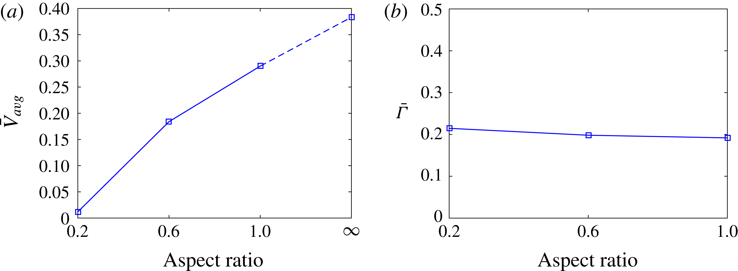
As the span of the panel increases, the swimming performance increases. In figure 17(a) the swimming speed was found be highest for the two-dimensional panel, with swimming speed for the three-dimensional cases approaching this level as the span length increased. Measuring the circulation of the tips for the three-dimensional cases (figure 17 b), we found the circulation measured increases slightly as the span decreases, where the panel with an aspect ratio of 0.2 has an 8 % increase circulation relative to the reference panel. This suggests that the additional drag generated from the tip vortices plays a relatively larger role as the span decreases.
3.6 Comparison between tethered and free-swimming panels
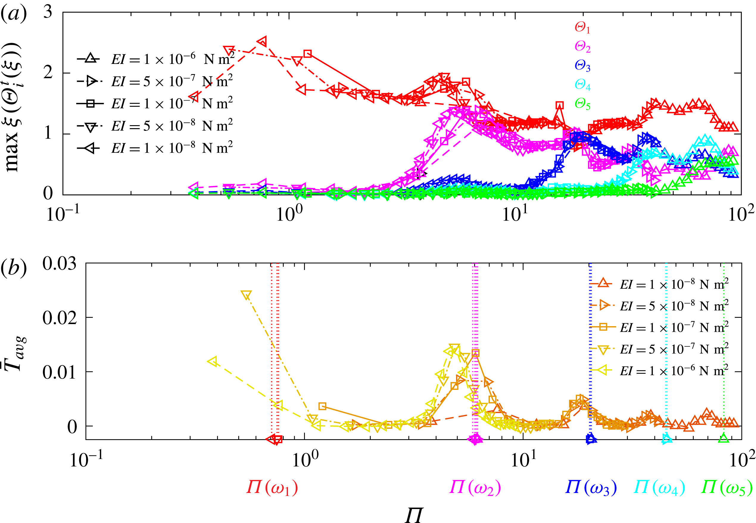
Do the peaks in the swimming speeds of an actuated, untethered panel correspond to the peaks in the thrust generated by the same actuated panel that is tethered and not free to swim? To examine this, we performed a set of simulations of tethered panels at the same heaving frequencies and five bending moduli as in untethered simulations. In this set of simulations, a tethered body force was applied to the leading edge and the panel was heaved until its motion reached a steady state. Figure 18(a) shows the maximum modal contributions of the first five modes computed from the emergent geometries of the tethered panels. We find that the peaks in these modal contributions correspond to the peaks observed for the freely swimming panels shown in figure 6(c). In addition, for these tethered panels the resulting forces
 ${\mathcal{F}}$
from the heaving motion were recorded and used to compute the resulting non-dimensional forward thrust
 $\bar{T}$
. This thrust was then averaged over a heaving cycle (
 $\bar{T}_{avg}$
). Figure 18(b) shows the thrust developed by each of the five tethered panels as a function of the effective flexibility. We find that peaks in
 $\bar{T}_{avg}$
occur near the same values of effective flexibility that displayed peaks in forward swimming speed for the corresponding untethered simulations (see figure 4
c). These peaks in turn correspond to local peaks in the modal contributions.
(a) Plot of the maximum modal contribution of each mode as a function of the tethered, heaving panels’ effective flexibility. Higher mode contributions increase as effective flexibility increases. (b) Plot of the dimensionless thrust,
 $\bar{T}_{avg}$
, as a function of the effective flexibility,
 $\unicode[STIX]{x1D6F1}$
. The effective flexibilities corresponding to the analytic prediction of the first five harmonic response frequencies (Van Eysden & Sader Reference Van Eysden and Sader2007) for the five panels are indicated by symbols on the horizontal axis, from which emanate dashed vertical lines whose colour corresponds to the five modes in panel (a).
We also use the tethered panel framework to validate our simulation results by comparing predictions of peaks in thrust with analytical approximations from a linearized theory. Van Eysden & Sader (Reference Van Eysden and Sader2006, Reference Van Eysden and Sader2007, Reference Van Eysden and Sader2009) developed a theory for the frequency response of a cantilever beam with rectangular cross-section immersed in a viscous fluid. In that study the fundamental frequencies are a function of panel geometry,
 $EI$
and Reynolds number, and are based on the exact solution of the linearized Navier–Stokes equations produced by a zero-thickness, infinitely long oscillating blade. It is noted in Van Eysden & Sader (Reference Van Eysden and Sader2007) that these approximations to harmonic response frequencies become less accurate as the mode increases due to the heightened three-dimensional aspects of the cantilever–fluid system. As a way of validating our method, we compare the frequencies at which the tethered panels of our simulations achieve local peaks in thrust to the values of harmonic response frequencies corresponding to different modes predicted by Van Eysden & Sader (Reference Van Eysden and Sader2007). For each of our five panels with fixed geometry and different bending moduli
 $EI$
, we compute the harmonic response frequencies
 $\unicode[STIX]{x1D714}_{n}$
associated with mode
 $n$
using the linear theory. For that
 $\unicode[STIX]{x1D714}_{n}$
and
 $EI$
, we associate an effective flexibility
 $\unicode[STIX]{x1D6F1}$
of that panel waved at the harmonic response frequency. These effective flexibilities (for five panels and the first five modes) are indicated on the horizontal axis of figure 18(b), and vertical lines are drawn emanating from these values. For each mode
 $n$
, the theoretical values of effective flexibility are essentially equal for the different bending moduli. For the smallest values of
 $\unicode[STIX]{x1D6F1}$
that correspond to stiff panels or panels heaved at low frequencies, restrictive computational costs do not allow simulations that resolve the first mode, so we focus on modes 2–5. However, the effective flexibility corresponding to the theoretical harmonic response frequency of the second mode for
 $EI=1\times 10^{-7}$
and
 $5\times 10^{-8}~\text{N}~\text{m}^{2}$
differs from the simulation value of
 $\unicode[STIX]{x1D6F1}$
at which peaks occur by less than 0.3 %, and for the third mode by less than 10 %. Larger differences are associated with higher modes, as expected. For stiffer panels,
 $EI=1\times 10^{-6}$
and
 $5\times 10^{7}~\text{N}~\text{m}^{2}$
, the computed effective flexibilities for mode 2 are approximately 22 % lower than those predicted by the analytic model of Van Eysden & Sader (Reference Van Eysden and Sader2007). The least stiff panel,
 $EI=1\times 10^{-8}~\text{N}~\text{m}^{2}$
, corresponds to a relative difference of 30 % in effective flexibilities for mode 2. The agreement between the harmonic response frequencies for modes 2 and 3 estimated by two-dimensional linear theory and those computed using the full three-dimensional Navier–Stokes system serves as a validation of the simulations.
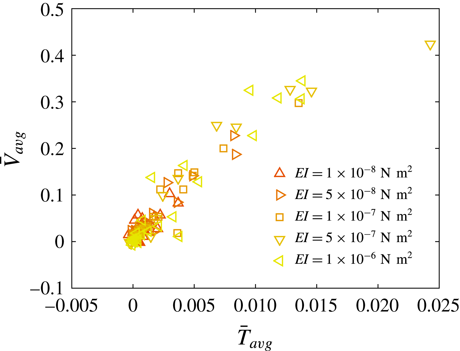
Figure 19 show scatter plots of the thrust of a tethered heaving panel and the speed of its untethered counterpart (
 $\bar{T}_{avg}$
,
 $\bar{V}_{avg}$
), for the five panels. We find that for tethered panels that produce positive thrust,
 $\bar{T}_{avg}$
, increasing thrust generally corresponds to increasing free-swimming speed
 $\bar{V}_{avg}$
. To further examine the differences between tethered and untethered panels, we examined the modal contributions of the tethered panels (figure 18
a). We find that the amplitude of modal contributions of the panels have peaks at the same
 $\unicode[STIX]{x1D6F1}$
value, although the amplitude of the modal contribution varies.
Plot of the maximum modal contribution of each mode with respect to the heaving panels’ effective flexibility. Higher mode contributions increase as effective flexibility increases.
4 Discussion
In this study, we developed a model of a three-dimensional, flexible panel that is heaved sinusoidally at its leading edge in a viscous fluid and used numerical simulations to study the role of resonance, fluid forces and shape evolution in the propulsive performance of the panels. As in previous experimental work on tethered panels (Quinn et al. Reference Quinn, Lauder and Smits2014b ), we found that the effective flexibility captures the main features of the elastohydrodynamic system. Even when the material properties differ substantially, panels flapping at different frequencies can have the same effective flexibility. In this case, they exhibit similar deformation patterns, both in shape and phase. This leads to similar flow patterns, which in turn result in similar non-dimensional swimming speeds.
However, there are important differences that correspond to the material properties. At the same effective flexibility, more flexible panels (lower
 $EI$
) are more economical: they require less input power to swim at about the same dimensionless speed, even when the effective flexibility is approximately the same. Conversely, stiffer panels (higher
 $EI$
) swim at Strouhal numbers closer to the range associated with high propulsive efficiency (Triantafyllou, Triantafyllou & Grosenbaugh Reference Triantafyllou, Triantafyllou and Grosenbaugh1993; Taylor et al.
Reference Taylor, Nudds and Thomas2003). These differences may correspond to the Reynolds number
 $Re_{in}$
, which is higher for stiffer panels at the same effective flexibility. This corresponds to a more complex wake, with higher forces on the panel, which leads to a greater forward speed for a given actuation, but also takes more input power and thus results in a lower economy. Similarly, our observations on how flexibility can increase the swimming economy of the panel (figure 5
b) coincide with the observations by Dewey et al. (Reference Dewey, Boschitsch, Moored, Stone and Smits2013) that found an increase in propulsive efficiency with the addition of flexibility.
As effective flexibility
 $\unicode[STIX]{x1D6F1}$
increases, there are multiple resonant peaks in performance parameters, including tailbeat amplitude (figure 4
a), swimming speed (figure 4
c), thrust (figure 18
b), along with measures of swimming energetics, including economy (figure 5
b) and inverse Strouhal number (figure 5
c). By decomposing the deformation into the fundamental beam bending modes, we found that each successive peak as
 $\unicode[STIX]{x1D6F1}$
increases corresponds to a peak in amplitude of a higher-order bending mode (figure 6
c). This confirms the observations of de Sousa & Allen (Reference de Sousa and Allen2011), that higher mode contributions have a larger amplitude as the bending rigidity of the panel decreases and heaving frequency remains constant. For a fixed effective flexibility, varying the heaving frequency requires that we proportionally adjust the bending rigidity to the order
 $1/2$
. This aligns with the findings of Michelin & Llewellyn Smith (Reference Michelin and Llewellyn Smith2009), who detailed how the resonant frequency associated with each mode evolves as a function of bending rigidity.
The effective flexibility captures the presence of these resonant interactions, but the exact value differs for panels with different bending modulus. For instance, the curves in figure 4(c) do not collapse exactly. It is important to point out that although panels have similar effective flexibilities, the resulting dimensional swimming speed varies and can in turn adjust the location of the observed resonant peak (Quinn et al. Reference Quinn, Lauder and Smits2014b ). Another possibility for this discrepancy is that the approximation does not fully account for additional fluid drag terms when considering the solution to the Euler–Bernoulli beam equation (2.14) (Paraz et al. Reference Paraz, Eloy and Schouveiler2014; Richards & Oshkai Reference Richards and Oshkai2015). We also note that the panels in this study are neutrally buoyant and that additional inertial terms due to mass of the panel could lower the observed performance gain due to resonance, as was observed in Yeh & Alexeev (Reference Yeh and Alexeev2014).
The locations of the resonant peaks match well with those in the experimental study by Quinn et al. (Reference Quinn, Lauder and Smits2014b
). Because their study and ours differ in substantial ways, this correspondence in effective flexibility supports it as a good non-dimensional parameter for the fluid–panel system. In their study, the panel was tethered and a steady-state background flow was present, with
 $Re$
ranging from
 $7800$
to
 $46\,800$
, with the characteristic velocity chosen to be the steady-state background flow velocity. Our study focused on the propulsive performance of an untethered panel in quiescent flow, with the maximum
 $Re$
of
 $1500$
, using the highest observed swimming speed as the characteristic velocity. Although the range of
 $\unicode[STIX]{x1D6F1}$
values was similar to that of Quinn et al. (Reference Quinn, Lauder and Smits2014b
), the bending moduli of their panels were orders of magnitude higher than in our study.
We also find that for tethered panels that produce positive thrust
 $\bar{T}_{avg}$
, increasing swimming speeds
 $\bar{V}_{avg}$
in untethered panels corresponds to increasing thrusts in the tethered panels. For the tethered panels in our study, there is no oncoming flow, while in most experimental studies (e.g. Quinn et al. (Reference Quinn, Lauder and Smits2014b
)) there usually is a flow. This difference should not affect the overall pattern of thrust as a function of flexibility (figure 18
b). Quinn et al. (Reference Quinn, Lauder and Smits2014b
) compared thrust for panels with the same effective flexibility at different oncoming flow speeds. While the bending mode shapes changed, the amplitude and thrust did not. Recently, Van Buren et al. (Reference Van Buren, Floryan, Wei and Smits2018) studied this effect specifically, and showed that the oncoming flow speed does not affect the way thrust changes as a function of frequency. They measured thrust production for tethered panels as they varied the oncoming flow speed over a wide range and found only small differences at different speeds, differences that were much smaller than the effect of changing foil stiffness or pitching frequency. In our simulations, we find that the positive thrust of the tethered panels corresponds linearly with the swimming speeds of the untethered panels. There were differences in the maximum modal contributions between the tethered and untethered panels, but the point in the phase where the peak modal contribution occurs is relatively unchanged. This is potentially due to the vortex structures generated during the heaving cycle that, in the tethered case, do not advect away from the panel, as would be the case with the presence of background flow, or when the panel is free to swim. This effect can be seen for the untethered panel depicted in figure 9, which shows the presence of pressure generated by the shed vortex structures near the panel’s trailing edge. This pressure contributes to positive axial flow near the panel, as was observed by Green & Smits (Reference Green and Smits2008). In the tethered case, the same vortex structures would have a stronger influence on the panel’s deflection at the trailing edge.
We demonstrated that the effective flexibilities at which the tethered panels achieve peaks in thrust compare very well with the analytical predictions of Van Eysden & Sader (Reference Van Eysden and Sader2009) for modes 2 and 3. It was noted that the harmonic response frequencies, which are derived using a linear approximation of the Navier–Stokes equations, do not necessarily correspond with the mechanical resonance exhibited by the trailing edge when a force is acting on the panels. We also note a small shift in the
 $\unicode[STIX]{x1D6F1}$
values where peak trailing edge amplitudes occur, but these values from our simulations agree closely with those of the experimental study of Quinn et al. (Reference Quinn, Lauder and Smits2014b
) could affect the added mass associated with the heaving panel. The panels in our study had bending moduli
 $EI$
that were generally a few orders of magnitude less than those used by Quinn et al. (Reference Quinn, Lauder and Smits2014b
) and also differ in aspect ratio. A recent study by Piñeirua, Thiria & Godoy-Diana (Reference Piñeirua, Thiria and Godoy-Diana2017) found differences in aspect ratio also yield shifts in the optimal frequencies for peak swimming speed and thrust.
The study by Alben et al. (Reference Alben, Witt, Baker, Anderson and Lauder2012), where two-dimensional, rectangular panels were heaved at their leading edge in an inviscid fluid, found panel swimming speed to be proportional to panel length to
 $-1/3$
power and bending rigidity to the
 $2/15$
power. Although Alben et al. did not directly examine the effective flexibility of their panels, they indirectly do so by adjusting the added mass and internal bending forces by varying the length and rigidity of the panel respectively. By increasing the length of the panel they increase its effective flexibility, and their observed decline in swimming speed corresponds to our observed decline in the peak swimming speeds associated with the resonant peaks at higher effective flexibilities. Similarly, increasing the bending rigidity of the panel corresponds to an decrease of the effective flexibility of the panel. Alben et al. (Reference Alben, Witt, Baker, Anderson and Lauder2012) also found that increasing the length of the panel or decreasing the rigidity also increased the wavenumber of the panel deflection, which corresponds to the addition of higher modal contributions as effective flexibility decreases.
Our results may help to explain some of the characteristics of biological propulsors. Lucas et al. (Reference Lucas, Johnson, Beaulieu, Cathcart, Tirrell, Colin, Gemmell, Dabiri and Costello2014) found that many flexible biological propulsors tend to have the most bending approximately 0.6 of the way down their length and tended to bend at an angle of
 $30^{\circ }$
. If we treat our panels as propulsors like those analysed by Lucas et al. (Reference Lucas, Johnson, Beaulieu, Cathcart, Tirrell, Colin, Gemmell, Dabiri and Costello2014), with a flexion ratio of 0.6, and compute the angle formed by the trailing edge of the panel with respect to the point of inflection,
 $\unicode[STIX]{x1D717}=\tan ^{-1}[(0.5a_{trail})/(0.6c)]$
, we find that panels of high swimming speeds had
 $\unicode[STIX]{x1D717}$
between
 $26^{\circ }$
and
 $40^{\circ }$
, which are within the flexion angle ranges observed by Lucas et al. (Reference Lucas, Johnson, Beaulieu, Cathcart, Tirrell, Colin, Gemmell, Dabiri and Costello2014). Qualitatively, the panels that had the most similar kinematics to those observed by Lucas et al. (Reference Lucas, Johnson, Beaulieu, Cathcart, Tirrell, Colin, Gemmell, Dabiri and Costello2014) were panels near the second resonant peak (
 $\unicode[STIX]{x1D6F1}$
from 3 to 6) with substantial contributions from the first two bending modes (see figure 20
a,b). We found that panels near this peak also had the highest dimensional speed (
 $V_{avg}$
) compared to panels of differing effective flexibilities (figure 20
c). These results could also explain the inverse relationship between the body size and tail beat frequency that was observed in fish swimming by Bainbridge (Reference Bainbridge1958). Our results also coincide with Root & Courtland (Reference Root and Courtland1999), who found that pitching rubber fish models tended to have more higher-order modes at high frequencies, where fish tend to damp out the higher-order modes to improve their swimming economy.
(a) Plots of the flexible propulsors of free-swimming animals, with red arrows pointing to the point of inflection, from Lucas et al. (Reference Lucas, Johnson, Beaulieu, Cathcart, Tirrell, Colin, Gemmell, Dabiri and Costello2014). (b) The profile of a panel, with
 $\bar{\unicode[STIX]{x1D714}}_{y}$
contours, whose effective flexibility is near the resonant peak associated with first and second modal contributions, circled in (c).
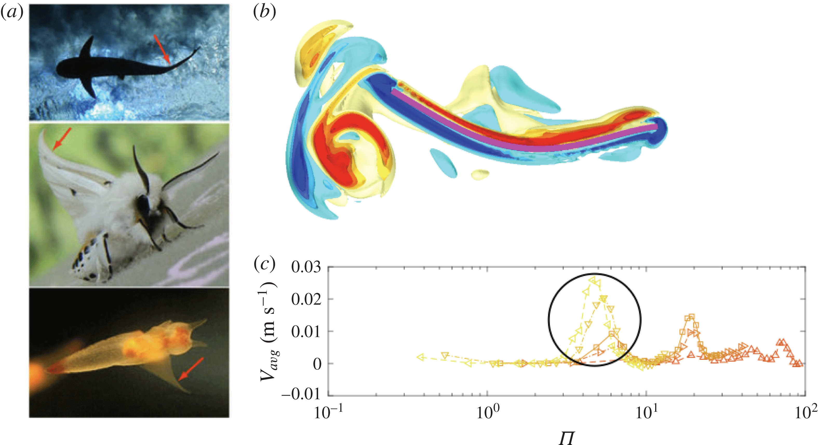
5 Conclusion
In conclusion, the development of this three-dimensional elastohydrodynamic model of a flexible panel allows for future investigations relating to flapping propulsion, such as the propulsive benefits to non-uniform flexibility (Liu & Bose Reference Liu and Bose1997; Lucas et al. Reference Lucas, Johnson, Beaulieu, Cathcart, Tirrell, Colin, Gemmell, Dabiri and Costello2014), non-sinusoidal heaving (Lehn et al. Reference Lehn, Thornycroft, Lauder and Leftwich2017) and variations in panel geometry (Buchholz & Smits Reference Buchholz and Smits2006; Van Buren et al. Reference Van Buren, Floryan, Brunner, Senturk and Smits2017). The numerical investigation reaffirms the validity of tethered panel experimental studies in studying the propulsive of performance of free-swimming bodies. This reduced model of a flexible flapping panel serves as major step towards a more comprehensive computational model of an undulatory swimmer that will couple neural activation, muscle mechanics and body elasticity to fluid dynamics. Such a comprehensive model will be capable of determining how the resulting kinematics measured from observational studies of swimming and flying organisms are a consequence of the interplay of muscle contractions and passive elastic properties of a body.
Acknowledgements
We would like to thank M. Leftwich for comments and suggestions during the preparation of this manuscript. We would also like to thank B. Griffith for advice on implementing the model in IBAMR. This work was supported by National Science Foundation grants DMS 1043626 (to A.P.H., R.C., L.J.F.), DBI-RCN 1062052 (to Avis H. Cohen and L.J.F.) and DMS 1312987 (to E.D.T. and L.J.F.).
Supplementary movies
Supplementary movies are available at https://doi.org/10.1017/jfm.2018.305.



