





1. Introduction
The interpretation of machine learning models (Molnar Reference Molnar2022) has become an increasingly important area of research. Its goal is to understand the behaviour of highly nonlinear models, such as Gradient Boosting Trees, Random Forests, and Neural Networks, that often involve complex feature interactions. Ultimately, interpretation seeks to answer questions such as “Why did the model produce a particular output?” (local explanations) and “What is the effect of variable
 $x_{i}$
on the model’s output?” (global explanations). In this talk, we focus on the latter, examining methods that improve our understanding of model behaviour. Such methods are essential for (i) building trust in model predictions, (ii) auditing models to detect spurious correlations, biases, and other undesirable behaviours, and (iii) generating scientific insight into the underlying phenomena captured by the models. Feature effect methods quantify how individual features influence model outputs across their value ranges. We briefly review established approaches and highlight weaknesses that can lead to inaccurate estimates. We then discuss recent advances, including regional effect plots, which generate feature effect plots for subregions of the feature space where heterogeneity is minimised. Finally, we present the Effector Python package, which implements these methods in an efficient and general-purpose framework.
2. A brief overview of feature effect methods
Given a “black-box” model
 $f: \mathscr{X} \rightarrow \mathscr{Y} $
, trained on a dataset
 $\mathscr{D}$
, feature effect methods aim at producing univariate (or bivariate) plots illustrating how a feature
 $x_{s}$
(or pair of features,
 $(x_{s}, x_{l})$
) influences the output of f for all values of
 $x_{s}$
(or all pairs of values
 $(x_{s}, x_{l})$
).
A popular feature effect method is Partial Dependence Plots (PDP) introduced by Friedman (Reference Friedman2001). PDPs essentially quantify the effect of
 $x_s$
by varying the feature value, while keeping all other features,
 $\mathbf{x}_c$
, to their original values, i.e.,
 \begin{equation} FE(x_s) = \mathbb{E}[f(x_s, \mathbf{x}_c)]\end{equation}
where the expectation is commonly estimated using the samples of the dataset
 $\mathscr{D}$
. Using this approach one can also produce Individual Conditional Expectation (ICE) plots, where the plot indicates how the model output changes with
 $x_s$
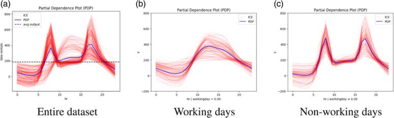
. An example of a PDP plot along with selected ICE plots is shown in Figure 1(a), for a model trained on the bike sharing dataset (Fanaee-T and Gama Reference Fanaee-T and Gama2013).
PDP (blue) and ICE plots (red) illustrating the effect of the “hour” feature on the number of bike rentals. In (a), the whole dataset is used, while in (b) and (c) we observe the PDP for working and non-working days respectively. These subregions (automatically identified using the algorithm proposed in (Gkolemis et al. 2023b)) lead to reduced heterogeneity of the feature effects.

Figure 1 Long description
Panel A: A partial dependence plot (PDP) and individual conditional expectation (ICE) plot showing the effect of the hour feature on bike rentals for the entire dataset. The x-axis represents the hour of the day, and the y-axis represents the number of bike rentals. The blue line indicates the PDP, while the red lines represent the ICE plots. The plot shows fluctuations in bike rentals throughout the day. Panel B: A partial dependence plot (PDP) and individual conditional expectation (ICE) plot for working days. The x-axis represents the hour of the day, and the y-axis represents the number of bike rentals. The blue line indicates the PDP, while the red lines represent the ICE plots. The plot shows a peak in bike rentals during morning and evening hours. Panel C: A partial dependence plot (PDP) and individual conditional expectation (ICE) plot for non-working days. The x-axis represents the hour of the day, and the y-axis represents the number of bike rentals. The blue line indicates the PDP, while the red lines represent the ICE plots. The plot shows peaks in bike rentals during midday and evening hours.
One problem with PDPs is that arbitrarily varying
 $x_s$
without changing
 $\mathbf{x}_c$
can lead to improbable (out of distribution) or even impossible samples, thus introducing bias in the estimation of effects. One solution (Apley and Zhu Reference Apley and Zhu2020) could be the conditioning of
 $\mathbf{x}_c$
on the value of
 $x_s$
, i.e.,
 $FE(x_s) = \mathbb{E}_{\mathbf{x}_c|x_s}[f(x_s, \mathbf{x}_c)]$
meaning that the expectation is over values of
 $\mathbf{x}_c$
that were observed along with the value of
 $x_s$
in the dataset. Even this approach is problematic, however, since it does not isolate the effect of each feature when there are feature interactions. If
 $x_s$
is correlated with one ore more features in
 $\mathbf{x}_c$
the effect of
 $x_s$
will not be estimated correctly.
Apley and Zhu (Reference Apley and Zhu2020) addressed these problems by introducing the Accumulated Local Effects (ALE) plot for feature effect estimation. ALE plots are defined as follows
 \begin{equation} FE(x_s) = \int_{x_{s, min}}^{x_s}\mathbb{E}_{\mathbf{x}_c|z}[ \frac{\partial f}{\partial x_s}(z, \mathbf{x}_c)] \partial z \end{equation}
while they are approximated as
 \begin{equation} \sum_k^{k_x} \underbrace{\frac{1}{|\mathscr{S}_k|} \sum_{i:\boldsymbol{x}^i \in \mathscr{S}_k} \underbrace{[f(z_k, \mathbf{x}^i_c) - f(z_{k-1}, \mathbf{x}^i_c)]}_{\text{point effect}}}_{\text{bin effect}}\end{equation}
where the approximation takes place over bins
 $\mathscr{S}_k$
of the feature space, and
 $z_k$
are the values of
 $x_s$
at the bin limits. This approach overcomes the problems of PDPs.
3. DALE, heterogeneity and RHALE
Despite the improvement introduced by ALE plots, the ALE approximation introduces some key limitations, namely (i) using wide bins can introduce significant bias, since the approximation depends on out-of-distribution samples, (ii) narrow bins can introduce bias in the estimation, when the number of samples is small, (iii) changing the bin size requires recomputing the ALE plot, which can be computationally expensive. These limitations were highlighted by Gkolemis et al. (2023a) who proposed the use of an alternative ALE approximation strategy for differentiable models (e.g., neural networks). The key idea is to replace the finite differences of the ALE approximation with exact derivatives i.e.,
 \begin{equation} FE(x_s) = \Delta x \sum_k^{k_x} \underbrace{\frac{1}{|\mathscr{S}_k|} \sum_{i:\boldsymbol{x}^i \in \mathscr{S}_k} \underbrace{[\frac{\partial f}{\partial x_s}(x_s^i, \mathbf{x^i_c})]}_{\text{point effect}}}_{\text{bin effect}} \end{equation}
A key advantage of this approach is that it can leverage hardware-accelerated auto-differentiation frameworks, such as PyTorch, Tensorflow or JAX, for the parallel pre-computation of the derivatives for all features. This allows the computation of ALE plots for all features and different bin sizes with minimal complexity. Furthermore, DALE does not suffer from bias due to out-of-distribution samples, since the point effects are estimated using only samples of the dataset. The reader is referred to (Gkolemis et al. 2023a) for details.
Using DALE, one can observe that in some cases varying the bin size leads to changes in the estimation of the feature effect, even in cases where the number of samples in each bin is significant. This is caused by the heterogeneity of point effects that are averaged to produce the overall feature effect, i.e., it is a form of aggregation bias. The following example, based on Goldstein et al. (Reference Goldstein, Kapelner, Bleich and Pitkin2015), shows this clearly. Consider the model
 \begin{equation} \begin{aligned} Y &= 0.2X_1 - 5X_2 + 10X_2 \mathbb{1}_{X_3 > 0} + \mathscr{E}\\ \mathscr{E} &\stackrel{i.i.d.}{\sim} \mathscr{N}(0,1), \quad X_1, X_2, X_3 \stackrel{i.i.d.}{\sim} \mathscr{U}(-1, 1) \end{aligned} \end{equation}
Although on average, the effect of
 $X_2$
on Y is zero, the point effect of
 $X_2$
is
 $\pm 5$
, depending on the value of
 $X_3$
. Given a dataset, the bin selection influences the estimated effect of
 $X_2$
, depending on the distribution of the values of
 $X_3$
in the bins.
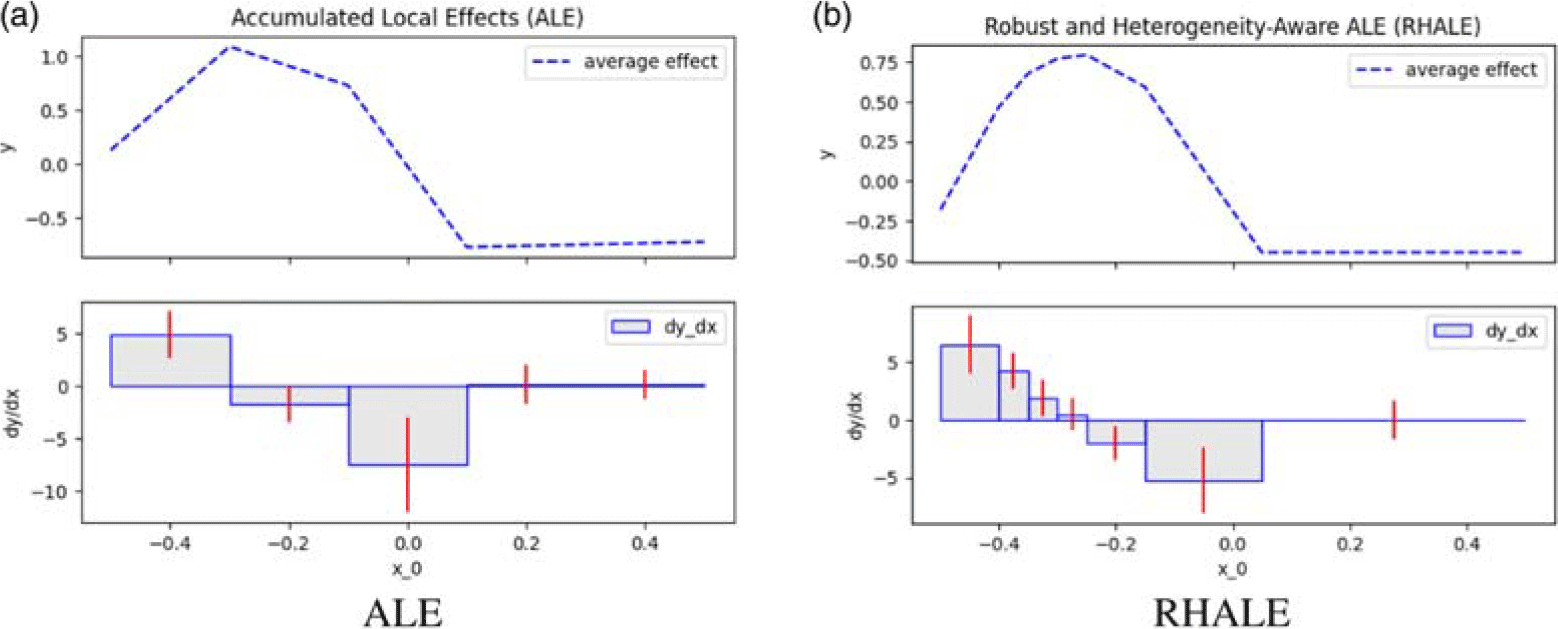
Such inconsistencies motivate the need to estimate the heterogeneity of effects, in addition to the average effect. Gkolemis et al. (2023b) proposed a method to estimate and approximate the heterogeneity of effects in ALE and explored the conditions under which these approximations are unbiased estimators of the heterogeneity. Furthermore, the conditions under which heterogeneity is minimised with a variable bin sizes were also identified. These observations motivated the development of a dynamic programming algorithm that allows the estimation of the optimal bin splitting, minimising heterogeneity and leading to robust ALE plots. Furthermore, it was proposed that the heterogeneity is also visualised along with the feature effect, to inform the user. An example of plots produced by the RHALE method is shown in Figure 2 (also from the Bike Sharing dataset).
Example comparing (a) ALE (with fixed bin size) with (b) RHALE (with optimal bin size). RHALE finds a variable bin splitting that minimises heterogeneity, leading to improved estimation of the feature effect (top plots)

4. Regional effect plots and the Effector Python package
RHALE produces optimal global feature effect plots, by selecting a bin splitting that minimises heterogeneity. Observing the example of Eq. (5), however, one can see that it is possible to further reduce heterogeneity and improve the estimation of feature effects by identifying subregions of the feature space where heterogeneity is reduced. In the example of Eq. (5), if one chooses to split the feature space into a region with
 $X_3 > 0$
and another with
 $X_3\leq 0$
, the effect of
 $X_2$
is computed as 5 and
 $-5$
, respectively, and the heterogeneity becomes zero. This idea of decomposing global effect plots was recently introduced by Herbinger et al. (Reference Herbinger, Wright, Nagler, Bischl and Casalicchio2024) (using the
 $\mathscr{H}-statistic$
).
These ideas motivate powerful strategies for producing regional effect plots that minimise heterogeneity. An example is shown in Figures 1 (b) and (c). The algorithm has identified that splitting the original feature space into a subregion with “working days” and another with “non-working days” significantly reduces heterogeneity, leading to these two regional effect plots. These new effect plots reveal that the effect of the “hour” feature is very different in these two subregions, offering valuable information about the underlying model.
Recently Gkolemis et al. (Reference Gkolemis, Diou, Ntoutsi, Dalamagas, Bischl, Herbinger and Casalicchio2024) released the Effector Python package, providing an efficient and general-purpose implementation of all the above global feature effect methods, as well as others, such as SHAP-DP and d-PDP. Moreover, the package includes the implementation of the regional counterparts of these methods, supporting automatic splitting strategies, while allowing users to control the number of subregions through hyperparameters. Importantly, for differentiable models, the package takes advantage of auto-differentiation capabilities of modern deep learning frameworks, leading to highly efficient feature effect computation.
5. Conclusion
Scientists who use machine learning with tabular data, including astrophysicists, can significantly benefit from feature effect methods and tools like Effector. These will allow them to go beyond treating their models as “black-box” predictive functions, allowing both model auditing and insights about the underlying phenomena. On the other hand, care must be taken to avoid aggregation and other biases, by (i) selecting appropriate feature effect estimation methods, (ii) visualising heterogeneity and (iii) using regional effect plots to minimise heterogeneity in each subregion.

 Open access

