I. INTRODUCTION
The ability to control magnetization by an external electric field or polarization by a magnetic field has promising technological applications. These include, among many others, spintronics, nonvolatile memories, Reference Velev, Jaswal and Tsymbal1 wireless energy transfer, Reference Pyatakov and Zvezdin2 multiple-state memory bits, and memories that can be written electrically and accessed magnetically. Reference Eerenstein, Mathur and Scott3 Similarly, piezoelectricity, where a uniform mechanical strain can induce an electric field and conversely, a uniform electric field can cause mechanical actuation, has also found wide applications, e.g., energy harvesting, artificial muscles, sensing and actuation, advanced microscopy, minimally invasive surgery among others. Reference Gautschi4–Reference Wang, Song, Zhang, He, Hu and Wang7
Historically, the magnetoelectric (ME) effect was predicted as early as 1894 while ME materials were not discovered until the 1950s. Since then, extensive research has gone into the quest for a strong ME effect. Disappointingly, the ME effect is intrinsic only in a few single phase materials and the coupling parameter itself (1–20 mV/cm Oe) is too small to be used effectively in several device realizations. Moreover, most of these materials have Curie or Neel temperature far below the room temperature. Growth of good crystals also represented a major challenge since it calls for expensive materials and processing techniques. Reference Ryu, Priya, Uchino and Kim8 As a result, the interest in ME effect declined, and all the applications which were foreseen at the time of its discovery were regarded as unpromising. Reference Fiebig9
The revival of this research field came in the 1990s where the focus shifted on engineering magnetoelectricity through composite materials. Reference Jahns, Piorra, Lage, Kirchhof, Meyners, Gugat, Krantz, Gerken, Knochel and Quandt22 An artificial way of designing ME materials may be realized using the concept of product properties; Reference Van Suchtelen10 that is, coupling magnetic and electric degrees of freedom indirectly through a third parameter such as mechanical deformation. Combining piezomagnetic and piezoelectric phases or magnetostrictive and piezoelectric phases can yield the desired property. Typically, in these composites, an external magnetic field creates mechanical strain in the magnetostrictive material, which is transferred to the adjacent piezoelectric material. Reference Shan, Lu, Wang and Majidi26,Reference Srinivasan29,Reference Ryu, Vazquez Carazo, Uchino and Kim31 This, in turn, generates an electric field due to the stress generated in the piezoelectric component of the composite. This way, magnetoelectricity can be engineered in materials which intrinsically do not allow the ME effect. Reference Fiebig9
While the field of piezoelectrics is more mature, most materials exhibiting a high electromechanical coupling are hard brittle ceramics such as perovskite ferroelectrics. Soft ME materials are virtually nonexistent and the few soft piezoelectric materials (e.g., polyvinylidene difluoride) are only weakly piezoelectric (as compared to crystalline, hard and brittle ferroelectrics). Multifunctional soft materials, with their attendant advantages of cost-effectiveness, ease of fabrication, and suitability for large deformation, can pave the way for a suite of applications, e.g., soft robotics and machines, flexible and stretchable electronics among others. Reference Anderson, Gisby, McKay, O’Brien and Calius11–Reference Suo13
While the phenomenon of magnetoelectricity alone is rather elusive, Reference Scott32 engineering the combined presence of both piezoelectricity and magnetoelectricity in soft materials, in amounts that are suitable for device applications, is a tall order. Reference Zhang, Leung, Kuang, Or and Ho33
In this work, based on our recent work on the concept of electrets in soft materials, Reference Liu and Sharma14,Reference Deng, Liu and Sharma15 we propose a mechanism that can be used to simultaneously create both a large (apparent) ME and piezoelectric effect. The soft materials neither have to be piezoelectric nor magnetostrictive.
The outline of this study is as follows. In Sec. II we briefly summarize the central concept while in Sec. III, we present the theory and formulation deriving all the necessary equations that fully describe the physical concept. In Sec. IV, we present the numerical solution of the governing equations and discuss the results. Finally, we conclude our work in Sec. V.
II. CENTRAL IDEA
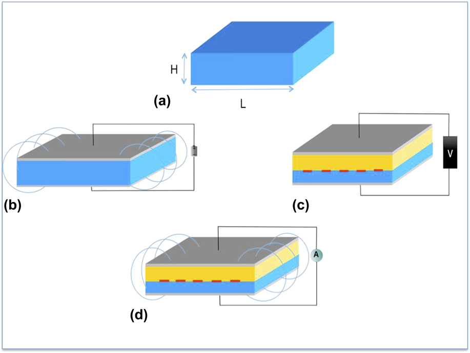
The central physical concept is depicted in Fig. 1. Consider first a soft homogeneous dielectric film as shown in Fig. 1(a). Neither intrinsic magnetoelectricity nor piezoelectricity exists since the material considered is homogeneous, nonpiezoelectric, and nonmagnetostrictive. Initially, the film is in an undeformed state. In Fig. 1(b), the film is sandwiched between two electrodes and exposed to an external electric field. The film will become polarized and because of the electric Maxwell stress, it will tend to compress. If now, an external magnetic field is imposed on this structure (where a pre-existing electric field exists), the magnetic Maxwell stress will deform the dielectric further, thus creating a change in the pre-existing electric field. The change in the pre-existing electric field due to the presence of the magnetic field manifests itself as the ME effect. This mechanism was recently proposed by Liu and Sharma. Reference Liu and Sharma14 Several interesting details are notable: (1) Engineering the ME effect, based on the nonlinear Maxwell stress concept, is universal in the sense that it occurs in all dielectric films and as a result, any dielectric material can be used. (2) For this mechanism to work, the material must be mechanically soft. This is understandable since the Maxwell stress is significant only for soft polymers. (3) There must exist a magnetic permeability mismatch between the dielectric film and ambient medium. This can be readily ensured by incorporating very minute amounts (negligible from a processing viewpoint) of highly permeable particles (e.g., soft magnetites). (4) Finally, the presence of a pre-existing electric field is required.
The central physical concept. (a) Visualize a homogeneous dielectric thin film, neither intrinsic magnetostriction nor piezoelectricity is assumed. (b) ME response of the dielectric thin film: first apply an external voltage, which deforms the film because of electric Maxwell stress. Then, a magnetic field is applied, which further deforms the film because of the magnetic Maxwell stress. This alters the pre-existing electric field. (c) Piezoelectric response of the electret material: a bilayer structure made of two polymers having different elastic properties with charge embedded at the interface is depicted. Under the application of an external voltage, this structure reveals an “apparent” piezoelectric behavior because of the electric Maxwell stress. (d) The structures in (b) and (c) are combined. The charges within the electret generate an electric field. Then, an external magnetic field is applied which will deform the material leading to a change in the pre-existing electric field. This structure will therefore exhibit both magnetoelectricity and piezoelectricity.
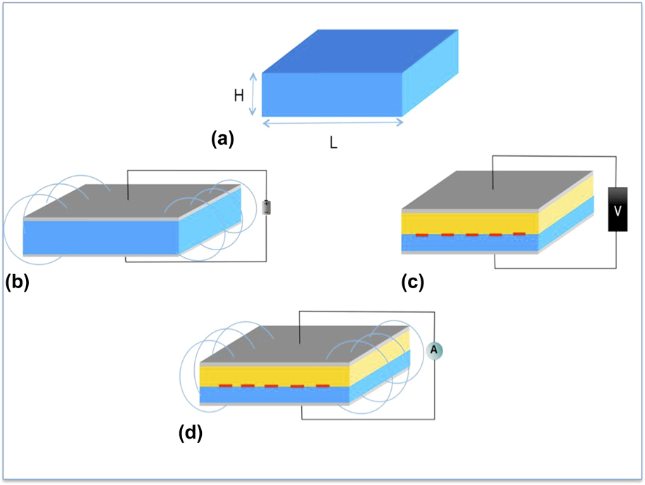
In Fig. 1(c), we consider two layers of nonpiezoelectric polymers. An electret material is created by incorporating charges and/or dipoles. Reference Harland, Brownell, Spector and Sun23 Among others, this can be accomplished in the following two ways: either by using layers of different materials with charges at the interfaces as in the figure, or by inserting voids in a uniform polymer matrix, i.e., using a foamy material containing charges on the void surfaces. Reference Deng, Liu and Sharma15,Reference Gerhard-Multhaupt21
Such electret states have been found to be (surprisingly) stable – specifically in certain kinds of polymer foams. Reference Qu and Yu24 The electret material behaves like an apparent piezoelectric material as long as the elastic properties in the material are nonuniform. Reference Eberle, Schmidt and Eisenmenger25,Reference Hillenbrand and Sessler30 The mechanism, reminiscent of the ME effect discussed in the preceding paragraphs is also based on the nonlinear Maxwell stress effect – deformation of the sample, induces a change in its pre-existing macroscopic polarization manifesting as an apparent piezoelectric effect. Indeed, experimentally, a two-way linear coupling between stress-electric fields has been shown for such electret materials even though microscopically the cause is the Maxwell stress effect rather than any intrinsic piezoelectric property. Reference Hillenbrand and Sessler16,Reference Bauer, Gerhard-Multhaupt and Sessler17 Polypropylene foams, with fairly stable electret configurations, have been fabricated that exhibit an apparent piezoelectric coefficient six times that of ceramic PZT. Reference Hillenbrand and Sessler16,Reference Bauer, Gerhard-Multhaupt and Sessler17
In Fig. 1(d), we combine the previous two cases. This is the central theme of the current study. Instead of a pre-existing applied voltage on a homogeneous material subject to a magnetic field, we consider a heterogeneous electret material subject to an external magnetic field. The presence of deposited charges inside the soft material will act as an alternative way of applying an electric field – albeit a nonuniform one. The magnetic Maxwell stress will tend to compress the two layers. This in turn will alter the electric field due to the presence of static charges. As a result, a ME effect will be created. In this scheme, we note that an external voltage need not be present for the ME effect to occur. Evidently, as discussed in the case of Fig. 1(c), a piezoelectric will also be present. In other words, Fig. 1(d) represents, schematically, a simple way to create simultaneous ME and piezoelectric effect in soft materials. In the following, we present a quantitative explanation of our central idea and a nonlinear theory that can be utilized to design such materials.
III. THEORY AND FORMULATION
To derive the governing equations, we consider the simplest possible configuration of an electret material: two layers of soft materials with charges embedded at the interface. The materials forming the two layers are assumed to be elastically nonlinear, but electrostatically and magnetostatically linear. We will assume in this context that each constituent material forming the electret structure is isotropic, a valid assumption for soft polymers. The constitutive relations of each of the films are given by
 $${\tilde \Sigma _{{\rm{mech}}}} = {{\partial {W_{{\rm{elst}}}}\left( F \right)} \over {\partial F}}{\rm{;}}\;{\bi{e}} = {p \over {{\varepsilon _0}\left( {{\varepsilon _{\rm{r}}} - 1} \right)}}{\rm{;}}\;{\bi{h}} = {{\bi{m}} \over {{\mu _{\rm{r}}} - 1}}\quad {\rm{,}}$$
where
 ${\tilde \Sigma _{{\rm{mech}}}}$
,
e
, and
h
are respectively the mechanical Piola–Kirchoff stress, electric field, and magnetic field;
F
,
p
, and
m
denote the deformation gradient, polarization, and magnetization, respectively. W
elst(
F
) stands for the elastic energy density, and μr and εr correspond to relative magnetic permeability and electric permittivity, respectively.
For the sake of simplicity, we assume that the electrodes are mechanically trivial, and they maintain a constant voltage difference across the films. Assuming the layers to be thin, the electric field in the ambient medium can be safely neglected. Moreover, the magnetic field is considered uniform in the films. Two different sets of coordinates will be used for each layer to maintain the distinction between the reference and the current configurations: (X, Y, Z) are the Lagrange coordinates of the material points and (x, y, z) are the Euler coordinates.
In this section, we proceed as follows: First, we present the case of a single soft material layer subject to electric and magnetic fields, as explained above, then we extend our results to the elastically heterogeneous electret structure taking into consideration the appropriate boundary conditions.
For simplicity, we make the following kinematic assumptions, χ = χ(X, Y, Z):
 $$x = X + u\left( X \right){\rm{;}}\;y = Y\left( {1 + {\varepsilon _y}\left( X \right)} \right){\rm{;}}\;z = Z\left( {1 + {\varepsilon _z}\left( X \right)} \right)\quad {\rm{.}}$$
u,ε y ,ε z :(0,L) → ℛ are scalar functions describing the deformed state of the film. The stretches in the X, Y, Z directions respectively are given by
 $${\lambda _x} = 1 + {{\partial u} \over {\partial X}};\;{\lambda _y} = {{\partial y} \over {\partial Y}} = 1 + {\varepsilon _y};\;{\lambda _z} = {{\partial z} \over {\partial Z}} = 1 + {\varepsilon _z}\quad {\rm{.}}$$
We denote the deformation gradient by F = Gradχ and the Jacobian measuring the change in the volume by J. In the current configuration, the polarization p and the magnetization m are related to the ones defined in the reference configuration by Reference Liu and Sharma14,Reference Liu18
 $${\bi{p}} = {{\tilde {\bi{P}}} \over J}{\rm{,}}\;{\bi{m}} = {{\tilde {\bi{M}}} \over J}\quad {\rm{.}}$$
We assume that x(0) = 0 and x(H) = h. The electric field and magnetic field in the current configuration must satisfy the Maxwell equations with the following boundary conditions:
 $${\rm{div}}\left( { - {\varepsilon _0}\,{\rm{grad}}\,\xi + {\bi{p}}} \right) = 0 {\rm{div}}\left( { - {\rm{grad}}\,\zeta + {\bi{m}}} \right) = 0 \xi \left( {x = l} \right) = V{\rm{,}}\,\xi \left( {x = 0} \right) = 0\,{\rm{and}}\, - {\rm{grad}}\,\zeta \to {{\bi{h}}^{\rm{e}}}\,{\rm{for}}\,x \to \infty \quad {\rm{,}}$$
where ξ is the electric potential field, ζ is the magnetic potential field, and h e is the external applied magnetic field.
The stored energy density function of the material is Reference Minlin19,Reference Toupin20
 $$\psi \left( {{\bi{F}}{\rm{,}}\tilde {\bi{P}}{\rm{,}}\tilde {\bi{M}}} \right) = {W_{{\rm{elst}}}}\left( {\bi{F}} \right) + {{{{\left| {\tilde {\bi{P}}} \right|}^2}} \over {2{\varepsilon _0}\left( {{\varepsilon _{\rm{r}}} - 1} \right)J}} + {{{\mu _0}{{\left| {\tilde {\bi{M}}} \right|}^2}} \over {2\left( {{\mu _{\rm{r}}} - 1} \right)J}}\quad {\rm{.}}$$
The first term on the right hand side refers to the elastic energy density whereas the second and third terms describe the contributions of the existence of polarization and magnetization to the total stored potential energy density. The central idea does not depend on the choice of the elasticity model. For illustration, we use the Neo-Hookean hyperelasticity model, which models polymers with very limited compressibility: Reference Treloar34
 $${W_{{\rm{elst}}}} = {\mu \over 2}\left[ {{J^{ - {2 \over 3}}}\left( {\lambda _x^2 + \lambda _y^2 + \lambda _z^2} \right) - 3} \right] + {k \over 2}{\left( {J - 1} \right)^2}\quad {\rm{,}}$$
where μ and κ stand respectively for the shear and bulk moduli.
Taking the applied voltage and magnetic field into consideration, the total free energy of the system can be written as Reference Liu18,Reference Liu35
 $${1 \over {{L^2}}}F\left[ {\chi {\rm{,}}\tilde {\bi{P}}{\rm{,}}\tilde {\bi{M}}} \right] = \int\limits_0^H {\psi \left( {{\bi{F}}{\rm{,}}\tilde {\bi{P}}}{\rm{,}}\tilde {\bi{M}}} \right){\mathop{\rm d}\nolimits} X} + {{{\varepsilon _0}} \over 2}\int\limits_0^h {{\lambda _y}{\lambda _z}{{\left| {{\rm{grad}}\,\xi } \right|}^2}{\mathop{\rm d}\nolimits} x} + \left. {V{\lambda _y}{\lambda _z}\left( { - {\varepsilon _0}{\rm{grad}}\,\xi + {\bi{p}}} \right)} \right|_{x = 0}^{x = h} + \int_0^h {{\lambda _y}{\lambda _z}{{{\mu _0}} \over 2}{{\left| {{\rm{grad}}\,{\zeta ^{{\rm{self}}}}} \right|}^2}{\mathop{\rm d}\nolimits} x} - \int_0^h {{\lambda _y}{\lambda _z}{\mu _0}{{\bi{h}}^{\rm{e}}} \cdot {\bi{m}}\;{\mathop{\rm d}\nolimits} x} \quad {\rm{,}} \cr}$$
where −gradζself = −gradζ − h e is the self magnetic field induced by the film alone. We remark that the self-field outside the film vanishes because of the thin-film geometry.
The equilibrium state of the film follows from the principle of minimum free energy. Therefore, the following variational problem is used: Reference Minlin19,Reference Toupin20
 $${\rm{mi}}{{\rm{n}}_{\left( {\chi {\rm{,}}\tilde P{\rm{,}}\tilde M} \right)}}F\left[ {\chi {\rm{,}}\tilde {\bi{P}}{\rm{,}}\tilde {\bi{M}}} \right]\quad {\rm{.}}$$
Carrying out the appropriate variational calculations with respect to deformation, polarization and magnetization
 $\left( {\chi {\rm{,}}\tilde {\bi{P}}{\rm{,}}\tilde {\bi{M}}} \right)$
yields three equilibrium Euler–Lagrange equations. In particular, we find that the equilibrium polarization and magnetization satisfy the following relations in the current configuration:
 $$\;{\bi{p}} = - {\varepsilon _0}\left( {{\varepsilon _{\rm{r}}} - 1} \right){\rm{grad}}\,\xi {\bi{m}} = \left( {{\mu _{\rm{r}}} - 1} \right)\left( { - {\rm{grad}}\,{\zeta ^{{\rm{self}}}} + {{\bi{h}}^e}} \right)\quad {\rm{,}} \cr}$$
which are consistent with Eq. (1) as expected. Inserting these two relations back in the Maxwell equations (5), we find the following expressions for the electric field and polarization:
 $$- {\rm{grad}}\,\xi = - {V \over h}{{\bi{e}}_x} {\bi{p}} = - {\varepsilon _0}\left( {{\varepsilon _{\rm{r}}} - 1} \right){V \over h}{{\bi{e}}_x}\quad {\rm{.}} \cr}$$
Also, if an external magnetic field is applied along the x direction, the self magnetic field and magnetization for x ∈ (0, h) are given by
 $$- {\rm{grad}}\,{\zeta ^{{\rm{self}}}} = - {{{\mu _0} - 1} \over {{\mu _{\rm{r}}}}}h_x^{\rm{e}}{{\bi{e}}_x} {\bi{m}} = {{{\mu _0} - 1} \over {{\mu _{\rm{r}}}}}h_x^{\rm{e}}{{\bi{e}}_x}\quad {\rm{,}} \cr}$$
whereas if the magnetic field is applied along the y direction, we obtain:
 $$- {\rm{grad}}\,{\zeta ^{{\rm{self}}}} = 0 {\bi{m}} = \left( {{\mu _{\rm{r}}} - 1} \right)h_y^{\rm{e}}{{\bi{e}}_y}\quad {\rm{.}} \cr}$$
After some algebra, we can rewrite the free energy in terms of λ x = h/H and J as
 $${F \over {\mu H{L^2}}} = {\hat W_{{\rm{elst}}}}\left( {{\lambda _x}{\rm{,}}\;J} \right) - {J \over {2\lambda _x^2}}\;{\hat f^{{\rm{elect}}}} - {J \over 2}\;{\hat f^{{\rm{mgf}}}}\quad {\rm{,}}$$
with the following abbreviations used for convenience:
 $${{\hat f}^{{\rm{elect}}}} = {{{\varepsilon _0}{\varepsilon _{\rm{r}}}{V^2}} \over {\mu \,{H^2}}}{\rm{,}}\;{{\hat W}_{{\rm{elst}}}} = {1 \over \mu }{W_{{\rm{elst}}}} {{\hat f}^{{\rm{mgf}}}} = {{{\mu _0}} \over \mu }\left[ {{{{\mu _{\rm{r}}} - 1} \over {{\mu _{\rm{r}}}}}{{\left( {h_x^{\rm{e}}} \right)}^2} + \left( {{\mu _{\rm{r}}} - 1} \right){{\left( {h_y^{\rm{e}}} \right)}^2}} \right]\quad {\rm{.}} \cr}$$
Now, we extend the model to account for the electret material taking into consideration the appropriate boundary conditions. The equilibrium conditions are then found by minimizing the total free energy F T(λ1, λ2, J 1, J 2) of the system with respect to variables λ1, λ2 that stand respectively for the stretches in the x direction for the first and second layers, and J 1, J 2 that refer to the volume changes of layers 1 and 2:
 $${F_{\rm{T}}}\left( {{\lambda _1}{\rm{,}}{\lambda _2}{\rm{,}}{J_1}{\rm{,}}{J_2}} \right) = \int\limits_0^{{H_1}} {{\psi _1}\left( {{{\bi{F}}_{\bf{1}}}{\rm{,}}\widetilde {{{\bi{P}}_{\bf{1}}}}{\rm{,}}\widetilde {{{\bi{M}}_{\bf{1}}}}} \right){\mathop{\rm d}\nolimits} {X_1}} + \int\limits_0^{{H_2}} {{\psi _2}\left( {{{\bi{F}}_{\bf{2}}}{\rm{,}}\widetilde {{{\bi{P}}_{\bf{2}}}}{\rm{,}}\widetilde {{{\bi{M}}_{\bf{2}}}}} \right){\mathop{\rm d}\nolimits} {X_2}} + {{{\varepsilon _0}} \over 2}\int\limits_0^{{h_1}} {{{{J_1}} \over {{\lambda _1}}}{{\left| {grad\,{\xi _1}} \right|}^2}{\mathop{\rm d}\nolimits} {x_1}} + V{{{J_1}} \over {{\lambda _1}}}\left. {\left( { - {\varepsilon _0}{\rm{grad}}\,{\xi _1} + {{\bi{p}}_1}} \right)} \right|_{{x_1} = 0}^{{x_1} = {h_1}} + {{{\varepsilon _0}} \over 2}\int\limits_0^{{h_2}} {{{{J_2}} \over {{\lambda _2}}}{{\left| {{\rm{grad}}\,{\xi _2}} \right|}^2}{\mathop{\rm d}\nolimits} {x_2}} + V{{{J_2}} \over {{\lambda _2}}}\left. {\left( { - {\varepsilon _0}{\rm{grad}}\,{\xi _2} + {{\bi{p}}_2}} \right)} \right|_{{X_2} = 0}^{{x_2} = {h_2}} + \int\limits_0^{{h_1}} {{{{J_1}} \over {{\lambda _1}}}{{{\mu _0}} \over 2}{{\left| {{\rm{grad}}\,\zeta _1^{{\rm{self}}}} \right|}^2}{\mathop{\rm d}\nolimits} {x_1}} - \int\limits_0^{{h_1}} {{{{J_1}} \over {{\lambda _1}}}{\mu _0}{{\bi{h}}^{\rm{e}}} \cdot {{\bi{m}}_1}\,{\mathop{\rm d}\nolimits} {x_1}} + \int\limits_0^{{h_2}} {{{{J_2}} \over {{\lambda _2}}}{{{\mu _0}} \over 2}{{\left| {{\rm{grad}}\,\zeta _2^{{\rm{self}}}} \right|}^2}{\mathop{\rm d}\nolimits} {x_2}} - \int\limits_0^{{h_2}} {{{{J_2}} \over {{\lambda _2}}}{\mu _0}{{\bi{h}}^{\rm{e}}} \cdot {{\bi{m}}_2}\,{\mathop{\rm d}\nolimits} {x_2}} \quad {\rm{.}}$$
The boundary conditions emerge from the field equations imposed by Maxwell equations and the presence of the charges at the interface between the two materials:
 $$x\left( { - {H_2}} \right) = - {h_2}{\rm{;}}\;x\left( {{H_1}} \right) = {h_1} \xi \left( {X = 0} \right) = 0{\rm{;}}\;\xi \left( {X = {H_1}} \right) = {\xi _1}{\rm{;}}\;\xi \left( {X = - {H_2}} \right) = - {\xi _2} {\rm{div}}\left( { - {\varepsilon _0}{\rm{grad}}\,\xi + {\bi{p}}} \right) = \rho \left( x \right)\quad {\rm{.}}$$
The electric field along the e x direction in each of the layers is given by
 $${E_1} = - {{{\xi _1}} \over {{h_1}}}{\rm{;}}\;{E_2} = {{{\xi _2}} \over {{h_2}}}\quad {\rm{.}}$$
Consequently, we obtain:
 $${\xi _1} - {\xi _2} = V {D_1} - {D_2} = - {{{\varepsilon _1}{\varepsilon _0}{J_1}} \over {\lambda _1^2}}{{{\xi _1}} \over {{H_1}}} - {{{\varepsilon _2}{\varepsilon _0}{J_2}} \over {\lambda _2^2}}{{{\xi _2}} \over {{H_2}}} = {q_0}\quad {\rm{,}}$$
where D 1, D 2 are the electric displacement along the e x direction.
Using the above interface conditions for the electric field, we find expressions for ξ1, ξ2 which are later replaced in the governing equations:
 $$\eqalignb{ & {{{\xi _1}} \over {{H_1}}} = {{{\varepsilon _2}{J_2}\lambda _1^2V - \lambda _1^2\lambda _2^2{H_2}{q_0}} \over {{\varepsilon _1}{J_1}\lambda _2^1{H_2} + {\varepsilon _2}{J_2}\lambda _1^2{H_1}}} \cr & {{{\xi _2}} \over {{H_2}}} = {{ - {\varepsilon _1}{J_1}\lambda _2^2V - \lambda _1^2\lambda _2^2{H_1}{q_0}} \over {{\varepsilon _1}{J_1}\lambda _2^1{H_2} + {\varepsilon _2}{J_2}\lambda _1^2{H_1}}}\quad {\rm{.}} \cr}$$
As for the magnetic field boundary conditions, the following apply:
 $${\mu _{{{\rm{r}}_1}}}{\left( { - {\rm{grad}}\,{\zeta _1}} \right)_x} = {\mu _{{{\rm{r}}_2}}}{\left( { - {\rm{grad}}\,{\zeta _2}} \right)_x} {\left( { - {\rm{grad}}\,{\zeta _1}} \right)_y} = {\left( { - {\rm{grad}}\,{\zeta _1}} \right)_y}\quad {\rm{.}} \cr}$$
Minimizing (16), taking Eqs. (17)–(21) into consideration, we obtain the following governing equations:
 $$J_i^{ - {2 \over 3}}\lambda _i^4 - J_i^{{1 \over 3}}{\lambda _i} + {J_i}\hat f_i^{{\rm{elect}}} = 0 - {1 \over 3}\left( {J_i^{ - {5 \over 3}}\lambda _i^4 - J_i^{ - {2 \over 3}}{\lambda _i}} \right) + {{{\kappa _i}} \over {{\mu _i}}}\left( {{J_i} - 1} \right)\lambda _i^2 - {1 \over 2}\hat f_i^{{\rm{elect}}} - {1 \over 2}\hat f_i^{{\rm{mgf}}}\lambda _i^2 = 0\quad {\rm{,}}$$
where
 $$\hat f_i^{{\rm{elect}}} = {{{\varepsilon _i}{\varepsilon _0}} \over {{\mu _i}}}{\left( {{{{\xi _i}} \over {{{\rm{H}}_i}}}} \right)^2} \hat f_i^{{\rm{mgf}}} = {{{\mu _0}} \over {{\mu _i}}}\left[ {{{{\mu _{{r_i}}} - 1} \over {{\mu _{{r_i}}}}}{{\left( {h_x^{\rm{e}}} \right)}^2} + \left( {{\mu _{{r_i}}} - 1} \right){{\left( {h_y^{\rm{e}}} \right)}^2}} \right]\quad {\rm{,}} \cr}$$
i is an index which takes values of 1 and 2, used to denote each layer. Finally, the equilibrium state for the system can be found by solving the four equations in (22).
IV. RESULTS AND DISCUSSION
We present the full numerical solution for the four equations in (22). The materials chosen to illustrate the results are microporous polytetrafluoroethylene (PTFE) and polyvinylidene fluoride (PVDF). The material properties used in the calculations are listed below and can be found from the literature: Reference Wan, Xie and Zhong28,Reference Neugschwandtner, Schwodiauner, Bauer-Gogonea and Bauer36,Reference Kasprzyk, Motyl, Gajewski and Pasternak37
Layer 1:
 ${\mu _1} = 0.1\;{\rm{MPa,}}\;{\varepsilon _1} = 1.5{\varepsilon _0}{\rm{,}}\;{\kappa _1} = {{14} \over 3}{\mu _1}$
(corresponding to a Poisson ratio 0.4)
Layer 2:
 ${\mu _2} = 2\;{\rm{GPa,}}\;{\varepsilon _2} = 9.5{\varepsilon _0}{\rm{,}}\;{\kappa _2} = {{14} \over 3}{\mu _2}$
(corresponding to a Poisson ratio 0.4)
The magnetic permeability μr of both films is assumed to be 5. The typical value of this parameter, for most polymers, is close to unity. However, as stated earlier, even a minute amount of magnetite particles (which will have negligible mechanical consequences) can easily raise this value to 5 or larger (before magnetization saturation). The charge distribution at the interface is taken to 1 mC/m2, a typical value that can be realized experimentally.
Comparing the shear modulus for the two layers, it is found that the microporous PTFE layer is much softer than the PVDF layer. Thus, for the presented model, if the electret is deformed, the deformation will exist mostly within the soft layer. Equation (22) obviously indicates that the applied electric field
 $\tilde E$
which is along the x-direction, and magnetic field
 ${{\bi{h}}^e} = {\bi{h}}_y^{\rm{e}}{{\bi{e}}_y}$
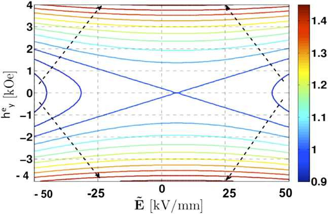
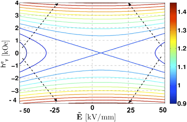
is coupled with the deformation. In Fig. 2, we present the strain contour plot with respect to the applied electric and magnetic fields. Here we only show the strain λ1 of the soft layer with respect to
 $\tilde E$
and
 $h_y^{\rm{e}}$
. The deformation is measured as the ratio of the deformed film thickness subsequent to the application of an external magnetic or electric field and the initial thickness of the film. The arrows indicate the direction in which the deformation increases. From the figure, it is interesting to observe that the effects of
 $\tilde E$
and
 $h_y^{\rm{e}}$
on the deformation are in an opposite sense to each other. The effect of
 $\tilde E$
is to compress the polymer film while
 $h_y^{\rm{e}}$
tends to stretch the film. It is worthwhile to mention that the contour plot is asymmetric about the line
 $\tilde E = 0$
because of the inserted charges at the interface. Calculations were performed for electric fields around 107 V/m, which is below the dielectric strength of both PVDF and PFTE (around 108 V/m).
Contour plot showing the deformation of the dielectric film as a function of the applied electric and magnetic fields.
Since the electric and the magnetic fields couple to each other through the deformation, it is also instructive to investigate the effective piezoelectric coefficient of the electret material in the presence of an external magnetic field. Recently, the piezoelectricity of electret structure was investigated.
Reference Deng, Liu and Sharma15
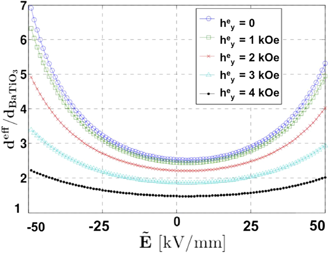
It was shown that for electric fields as high as 0.05 V/nm, the effective piezoelectric response obtained is around twice as that of the barium titanate (78 pC/N). In this context, we proceed with the calculation of the piezoelectric coefficient. This can be done by finding the difference between the change in the total thickness as a function of the change in the applied voltage for the two cases q
0 = 0 and q
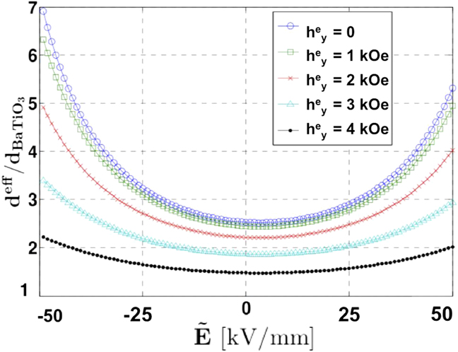
0 ≠ 0. Figure 3 shows the results for various magnetic fields applied. The apparent piezoelectricity of the electret structure is normalized by that of barium titanate. Because of the large deformation and the ensuring nonlinearity, the piezoelectric coefficient that depends on the applied field changes nonlinearly with respect to
 $\tilde E$
. With the increase of
 $\tilde E$
, the piezoelectric coefficient also increases. Recall that the effects of
 $\tilde E$
and
 $h_y^{\rm{e}}$
are in opposite direction, so, as is observed in Fig. 3, not only the piezoelectric response changes, but also its rate of change with respect to
 $\tilde E$
reduces with the existence of magnetic field.
Effective piezoelectricity of a soft electret material.
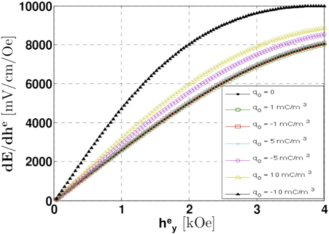
In Fig. 4, we show that the ME coupling of the electret is also affected by the inserted charges. In this case, we set the applied electric field
 $\tilde E$
to 107 V/m. The actual electric field E is calculated based on the deformation caused by the applied fields
 $\tilde E$
and
 $h_y^{\rm{e}}$
. The ME coupling constant dE/dh
e is affected by the interface charges. However, this effect is not significant when the charge density is below 1 mC/m3.
ME response of the soft electret material with different interface charges.
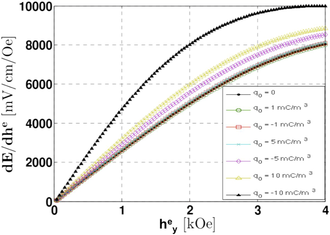
The presence of the interface charges can also be thought of as an alternative way of applying an electric field to the electret structure. The inserted charges generate their electric field within the material. Thus, when a magnetic field is applied, the deformation imposed by the magnetic Maxwell stress alters the internal electric field. As a result, a ME response is found. Notably, creating an electret structure allows the presence of a ME behavior even without the presence of an external voltage source.
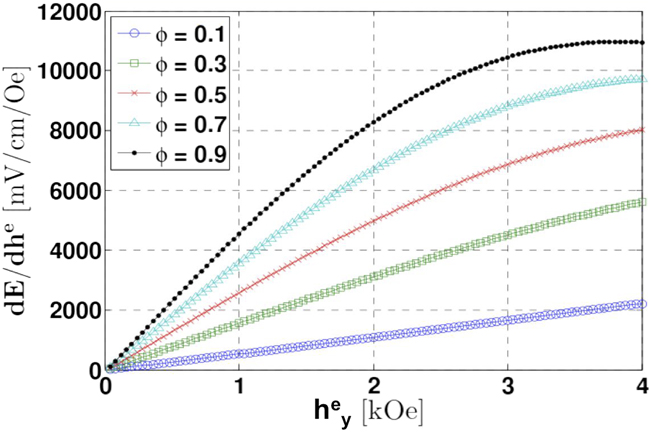
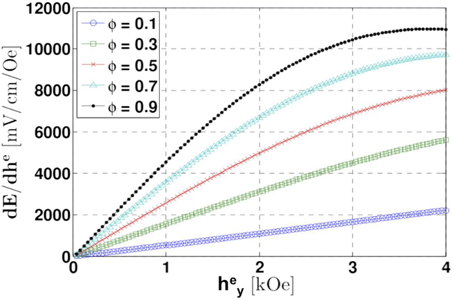
In Fig. 5, we study the impact of the volume fraction of the soft layer on the ME coupling behaviors of an electret. Figure 5 shows that as the volume fraction of the soft layer increases, the overall ME coupling constant dE/dh
e increases correspondingly. Evidently, the large deformation of the soft layer contributes significantly to the ME coupling. It is important to mention that this large deformation only exists in very soft materials such as the microporous PTFE used here. From this figure, we also find that for the cases with φ ≥ 0.5, dE/dh
e changes nonlinearly with respect to the applied magnetic field
 $h_y^{\rm{e}}$
.
ME response of the soft electret material with different ϕ.
Several implications may be drawn from our results. As seen in Fig. 2, we note that deformations as high as 40% can be achieved for high electric and magnetic fields. While not quite as large as elastomers, the contrast to ceramic-based analogous multifunctional materials is striking. Reference Zhao and Suo27 (The use of elastomers, unfortunately, does not appear to be practical since charges are unlikely to remain stable for too long in structures made from those.) How soft should the material be? The upper bound on Maxwell stress can reach roughly 105 Pa if we assume a typical magnetic field on the order of 104 Oe and electric field in the range of 106–108 V/m. This translates to about 10% strain induced in a dielectric with a Young modulus of around 1 MPa.
Moreover, this electret structure reveals a large apparent piezoelectric coefficient that depends nonlinearly on both the applied electric and magnetic fields. In other words, piezoelectric response can be modified with the application of an external field. The well-known and widely used piezoelectric ceramic material PZT has a linear piezoelectric constant around 290 pC/N which does not depend on any external conditions. Figure 3 shows that values of this magnitude can be realized for intrinsically nonpiezoelectric soft polymer structure by applying appropriate external fields. This comes with the advantage of large deformation that ceramic materials are incapable of. Taking into consideration the results of Fig. 5 that shows the dependence of the ME response on the volume fraction of the softer layer, the problem of choosing the appropriate materials for a device fabrication can be thought of as an optimization problem; picking the polymers that make up the electret structure and the corresponding volume fractions that yield the required piezoelectric or ME behavior.
V. CONCLUSION
We propose a relatively simple concept to design soft materials that simultaneously exhibit some rather contradictory properties not usually found in soft materials – apparent piezoelectricity and magnetoelectricity. Geometric nonlinearity and the presence of stable charges within the interfaces of the material is the key mechanism that couples mechanical, electric and magnetic fields. Our work is conceptual and we have illustrated our work using materials that have been experimentally shown to exhibit stable electret structures. Very large deformation may be possible by combining the concepts outline herein with the use of elastomers. However, the latter are likely to be quite vulnerable to charge leakage 38 – accordingly, experimental work that can find avenues to stabilize electret structures in elastomers is a promising research direction. Extension of our work to complex configurations and three-dimensional deformation states appears to be a tantalizing future direction that may pave the way for engineering and optimizing multifunctional material properties through electrets.
ACKNOWLEDGMENTS
Partial support from QNRF grant, NPRP: 6-282-2-119, is gratefully acknowledged. L. L. acknowledges the support of NSF CMMI-1238835, CMMI-135156, and AFOSRYIP-12.