





1. Introduction
While low-speed boundary layer (BL) control concepts are well developed, they are not easily applicable to hypersonic flight due to the harsh flight environments and the unique physics pertaining to hypersonic transition. Despite these challenges, there have been recent developments in control techniques feasible for implementation on hypersonic vehicles. Hypersonic transition control aims to dictate the state of the BL through passive and active control techniques. Active control techniques include forms such as wall suction and heat transfer. A subset of active control techniques includes reactive control, in which artificially produced, out-of-phase perturbations cancel out BL disturbances. This can be done through methods including periodic blowing or suction, heating, cooling or wall vibrations (Fedorov et al. Reference Fedorov, Malmuth, Rasheed and Hornung2001). Active control methods are difficult to implement in hypersonic vehicles due to their complexity. Kimmel (Reference Kimmel2003) suggests that the control techniques most promising for hypersonic flight are passive and non-reactive techniques, including porous coatings, local heating/cooling and vehicle shaping. Porous coatings are proven, both theoretically and experimentally, to delay hypersonic BL transition through mechanisms that attenuate the second-mode instability (Malmuth et al. Reference Malmuth, Fedorov, Shalaev, Cole, Hites, Williams and Khokhlov1998; Rasheed et al. Reference Rasheed, Hornung, Fedorov and Malmuth2002; Fedorov Reference Fedorov2003). The second Mack mode can be the dominant instability leading to transition for hypersonic vehicles that have low angles of attack, high lift-to-drag ratios, small free-stream disturbances, negligible surface roughness and predominantly two-dimensional hypersonic BLs. This was shown theoretically by Malik (Reference Malik1989) indicating that hypersonic laminar flow can be extended by the stabilisation of the second mode.
1.1. Early efforts in ultrasonic absorptive coating development
Malmuth et al. (Reference Malmuth, Fedorov, Shalaev, Cole, Hites, Williams and Khokhlov1998) assumed that an ultrasonic absorptive coating (UAC) would stabilise the second mode and demonstrated this through linear-stability theory. Fedorov et al. (Reference Fedorov, Malmuth, Rasheed and Hornung2001) explored this idea further by conducting a stability analysis for hypersonic BLs over porous walls with evenly spaced blind microholes. Results showed a reduction in second-mode growth rate due to absorption of disturbance energy by the porous coating through viscous action, consistent with the earlier analysis of Malmuth et al. (Reference Malmuth, Fedorov, Shalaev, Cole, Hites, Williams and Khokhlov1998). Rasheed et al. (Reference Rasheed, Hornung, Fedorov and Malmuth2002) performed experiments with a sharp cone outfitted with a porous coating made up of evenly spaced microholes, matching the surface from the computational analysis . These experiments showed transition location delay as much as 100 %. The exact transition location could not be characterised because the cone length was too short to obtain natural transition with the application of the porous coating. Similar experiments were conducted to represent random micro-structures typically seen on thermal protection systems (TPS) (Maslov et al. Reference Maslov, Shiplyuk, Sidorenko, Polivanov, Fedorov, Kozlov and Malmuth2006). Experiments investigated a sharp cone with a felt-metal coating at Mach-12. It was demonstrated for the first time that UAC of random structure delayed transition onset location up to 100 %.
Stability experiments were carried out on a sharp cone at Mach 5.95 for porous coatings of regular and random micro-structures reported on by Fedorov et al. (Reference Fedorov, Shiplyuk, Maslov, Burov and Malmuth2003, Reference Fedorov, Kozlov, Shiplyuk, Maslov and Malmuth2006). The UAC of regular microstructure was analogous to what was used in the experiments conducted by Rasheed et al. (Reference Rasheed, Hornung, Fedorov and Malmuth2002) and demonstrated stabilisation of the second mode with little effect on the first mode. The UAC application resulted in a measured maximum amplitude approximately 3 times lower than that measured on the solid wall. Further experiments were conducted with a felt-metal coating, which effectively stabilised the second-mode instability. However, it was seen that low-frequency disturbances were destabilised. Such destabilisation of low-frequency disturbances with the application of porous material appears to be an effect also observed in the current work. The experiments conducted by Rasheed et al. (Reference Rasheed, Hornung, Fedorov and Malmuth2002) were the first to quantitatively demonstrate the attenuation of the second-mode waves using UACs and showed a small destabilisation at low frequencies. The unexpected enhancement of the low-frequency disturbances motivated Chokani et al. (Reference Chokani, Bountin, Shiplyuk and Maslov2005) to perform a bispectral analysis to identify the nonlinear mechanism possibly triggered by the UAC. This analysis showed nonlinear phase locking in the presence of the porous walls, but not in the presence of the smooth surface. The effect was small and involved only the first mode, while not impacting the stabilising characteristics of the porous material. It was also shown that the harmonic resonance, which was pronounced on the smooth surface in its later stages, was suppressed completely on the side of the porous coating.
1.2. Recent efforts in UAC development
Wang & Zhong (Reference Wang and Zhong2012) explored the stabilisation of a Mach 5.92 BL via porous coatings with an emphasis on the effect of porous coating location and the destabilisation of the first mode. Stability simulations were conducted by placing felt-metal coatings locally along a flat plate surface. A relationship was discovered between disturbance stability dependent on material location relative to the synchronisation location. The porous coating was most effective at stabilising the BL when placed downstream of the synchronisation location.
Lukashevich, Morozov & Shiplyuk (Reference Lukashevich, Morozov and Shiplyuk2013) experimentally tested the effect of porous coatings of different lengths on a sharp cone at Mach 5.8 to assess their influence on second-mode instability. The results showed that varying the length of the material alters the second-mode suppression. The porous section with the longest length and closest to the nosetip resulted in second-mode destabilisation and the smaller lengths tested further downstream resulted in decreased second-mode amplitudes.
The effect of varying lengths and locations of UACs was further analysed by Poplavskaya, Reshetova & Tsyryulnikov (Reference Poplavskaya, Reshetova and Tsyryulnikov2019), who tested foam-nickel inserts mounted on flat plates at three streamwise locations. Inserts placed in the region of disturbance maximum provided the strongest attenuation of pressure-fluctuation amplitudes. Additional experiments comparing coatings with 80 and 160 mm lengths showed that longer inserts yielded greater suppression of disturbances. Overall, pressure pulsations on the surface of the plate with an application of porous material reduced pressure pulsations by 20 %–40 % depending on the angle of attack and the frequency of disturbances.
Similarly to the work done by Wang & Zhong (Reference Wang and Zhong2012), Lukashevich et al. (Reference Lukashevich, Morozov and Shiplyuk2013) and Poplavskaya et al. (Reference Poplavskaya, Reshetova and Tsyryulnikov2019), the current work shows a relationship between the location of the porous coating and the success of suppressing the second-mode instability.
To further explore the use of porous mediums, experiments carried out in the Mach 6 hypersonic wind tunnel at Peking University analysed the effect of permeable steel walls (Zhu et al. Reference Zhu, Shi, Zhu and Lee2020). PM-35, a permeable steel developed through powder particles, was manufactured as a flared cone geometry. Results suggest that the permeable steel delayed BL transition. The streamwise evolution of the second-mode waves on the porous wall increased faster, yet decayed at a slower rate than what was analysed on the smooth wall.
1.3. Ultrasonic absorptive coating development with carbon-based material
Recent research has been exploring the alternative material of carbon–fibre reinforced carbon-matrix ceramic (C/C) to achieve stabilisation of the second-mode instability. The C/C exhibits ultrasonically absorptive properties due to its natural porosity consisting of random micro-structures which is a common configuration used for TPS. The C/C represents an intermediate state of carbon-silicon carbide (C/C-SiC) which has been used as TPS on hypersonic vehicles (Turner et al. Reference Turner, Hörschgen, Jung, Stamminger and Turner2006; Weihs, Longo & Turner Reference Weihs, Longo and Turner2008) making this material promising as a candidate for hypersonic flight application. Experiments were done by Wagner et al. (Reference Wagner, Kuhn, Schramm and Hannemann2013) on a cone fitted with carbon-carbon ceramics at Mach 7.5. Results obtained from surface-mounted pressure sensors and heat transfer measurements showed the carbon-carbon ceramic effectively stabilised the second mode and increased the laminar portion of the BL over the porous surface.
Wartemann et al. (Reference Wartemann, Wagner, Kuhn, Eggers and Hannemann2015) explored the results from Wagner and used similar flow conditions to perform an linear-stability theory (LST) analysis while adapting the boundary conditions to account for the characteristics of the porous C/C material. The material’s ultrasonic absorption properties were investigated experimentally and theoretically to measure the reflection coefficient. These results were used to improve the BL conditions for the stability analysis above the porous surface. The original as well as the improved BL conditions were compared with the experimental results obtained by Wagner et al. (Reference Wagner, Kuhn, Schramm and Hannemann2013). It was shown that the improved conditions established by Wartemann et al. (Reference Wartemann, Wagner, Kuhn, Eggers and Hannemann2015) led to better agreement with the transition delay seen in Wagner’s experimental results.
Further analysis of conditions similar to Wagner’s experiments was explored by Sousa et al. (Reference Sousa, Wartemann, Wagner and Scalo2023) by conducting a direct numerical simulation of a spatially developing hypersonic BL over a cone’s surface. A complex broadband wall impedance was used to simulate the porous characteristics of the C/C surface. The findings show that, for the various flow conditions tested, the C/C attenuated the second-mode instability and delayed BL transition, as was seen in Wagner’s experimental results.
Experiments with a 3
 $^\circ$
half-angle cone were conducted in both the Boeing/AFOSR Mach 6 Quiet Tunnel (BAM6QT) at Purdue University and the hypersonic wind tunnel (H2K) at DLR in Cologne by Willems et al. (Reference Willems, Gülhan, Ward and Schneider2017), to explore the effect of UACs in low-disturbance, flight-like hypersonic flow compared with conventional tunnel conditions. Two porous materials were tested: the first was a porous surface of regular uniform blind holes with a porosity that closely matched the simulations conducted by Wartemann & Lüdeke (Reference Wartemann and Lüdeke2010). The second porous section was made of a C/C material with a natural random porosity. Both porous sections resulted in stimulation of second-mode amplitudes, leading to earlier transition, in contrast to previous results. The possible reasons for these conflicting results include lower second-mode frequencies produced by the 3
 $^\circ$
cone than that of the 5
 $^\circ$
and 7
 $^\circ$
cone used in previous experiments performed by Rasheed et al. (Reference Rasheed, Hornung, Fedorov and Malmuth2002), Fedorov (Reference Fedorov2011) and Wagner et al. (Reference Wagner, Kuhn, Schramm and Hannemann2013). A second reason may relate to the position and length of the porous surfaces as found by Wang & Zhong (Reference Wang and Zhong2012), Lüdeke & Wartemann (Reference Lukashevich, Morozov and Shiplyuk2013) and Lukashevich, Morozov & Shiplyuk (Reference Lukashevich, Morozov and Shiplyuk2016).
The most recent prior work in BAM6QT attempting the implementation of porous materials to attenuate the second-mode instability was Mamrol (Reference Mamrol2020) and Miller et al. (Reference Miller, Mamrol, Redmond, Jantze, Scalo and Jewell2022). A flat plate facilitated incorporation of porous C/C material formed in flat coupons, but the second mode was not detected on the control (solid, non-porous) flat plate under quiet flow conditions. Therefore, the flat plate model was not the ideal candidate to examine these effects in a low-disturbance environment where the dominant instability inputs are not free-stream noise. The current work is an improvement upon the aforementioned research with an updated geometry, lengthened to allow the natural development of the second-mode instability.
The paper is organised as follows: in § 2, the experimental set-up in the BAM6QT is outlined and model instrumentation and flow conditions are discussed. Section 3 describes the choice of porous materials, with the various configurations tested on the cone, and develops the ultrasonic characterisation of the foams to inform companion direct numerical simulation (DNS)/LST analysis. Section 4 details the computational set-up for the axisymmetric DNSs and linear-stability analysis. Section 5 presents experimental and computational results for a 3
 $^\circ$
cone, examining the effects of different Polyether ether ketone (PEEK)-carbon foam configurations on BL transition at varying free-stream Reynolds numbers. Finally, § 6 summarises the key findings of this experimental and computational investigation.
2. Experimental set-up
2.1. Model and instrumentation
Experiments were conducted with a sharp
 $3^\circ$
half-angle cone with an overall length of
 $109.1$
cm and a base diameter of
 $11.43$
cm. The cone is comprised of 6 parts – a steel nosetip, three modular test pieces, a base and a base extension. The dimensions for each section of the model can be seen in figure 1. All surfaces of the
 $3^\circ$
half-angle cone, apart from the steel nosetip, are made out of PEEK to facilitate infrared temperature measurements and heat transfer calculations. The nominally sharp steel nosetip was measured under a microscope to have a 50
 ${\unicode{x03BC}}$
m radius. The model is equipped with 22 surface-mounted PCB pressure sensors. There are 16 pressure sensor ports along the main array spanning the base and the base extension, all within the domain of dependence (Wang & Zaki Reference Wang and Zaki2025) of the three modular test pieces upstream. There are two sets of four azimuthally spaced sensor ports at x = 75.5 cm and x = 95.6 cm to allow for precision angle-of-attack measurements. The sensor locations are outlined in figure 1 and table 1.
Technical illustration of the 3
 $^\circ$
half-angle cone used throughout this work.

Axial location (
 $x$
-axis) and azimuthal position (
 $\theta$
-axis) of the PCB sensors. The main sensor array shown in figure 1 is located along the
 $\theta =0^{\circ }$
line.

2.1.1. Pressure sensors
The surface-mounted sensors used throughout the testing were PCB132B38 sensors made by PCB Piezotronics, Inc. These were chosen because they are capable of withstanding startup and shutdown forces produced by hypersonic test facilities and can measure high-frequency disturbances. These PCBs are high-pass filtered with an 11 kHz cutoff frequency and have a resonant frequency greater than 1 MHz. The high-pass filter excludes the measurements of the mean pressure and only accounts for pressure fluctuations. The exclusion of the mean pressure along with the large resonant frequency makes these sensors ideal for detecting second-mode frequencies, which are expected to be over 100 kHz. The piezoceramic sensing element has a diameter of 0.035 in. which is housed in a steel tube with a total diameter of 0.125 in. The sensing element is centred in the face ensuring the spatial accuracy of the pressure-fluctuation measurements. For the present work, factory calibrations provided by the manufacturer for each sensor were used to convert the voltage to pressure. The original purpose of these piezoelectric sensors was to detect the arrival of shocks, therefore, a single-point calibration provided by the factory is not as accurate for the amplitude of pressure-fluctuation measurements. It was determined by Berridge that the factory calibration had an attached magnitude uncertainty of up to 15 % (Berridge Reference Berridge2015). The stagnation pressure during a run is measured by a model ETL-79-HA-DC-190 Kulite pressure sensor. This Kulite is located upstream of the contraction on the inner nozzle wall where the flow is considered stagnant. A Paroscientific Inc. model 740 Digiquartz Portable Standard pressure gauge is used to measure the pressure of the driver tube section. This measured pressure is compared with the voltage measured by the contraction Kulite for different stagnation pressures. The contraction Kulite is calibrated through this comparison during each entry.
2.1.2. Infrared thermography
Infrared thermography (IR) is used throughout this work to make global heat transfer measurements. The IR data are of particular interest because they can be used to determine the state of the BL and give insights into the effectiveness of a UAC with respect to BL transition delay. Zaccara, Edelman & Cardone (Reference Zaccara, Edelman and Cardone2020) developed the current procedure employed in the BAM6QT to acquire heat transfer measurements using IR which involves reconstructing the IR images to acquire a map of the surface temperatures of the model. The BAM6QT IR set-up uses an Infratec ImageIR 8300 hp camera and a lens with a 12 mm focal length. A factory calibration was provided giving a temperature resolution of 0.02
 $^\circ$
K and accuracy of
 $\pm 1 ^\circ$
K. Data were collected at a 200 Hz frame rate with 1.5 s of pre-run images. An IR-transparent magnesium fluoride window was installed while performing IR measurements. This window measures a diameter of 4 inches, with an effective viewing area of 3.2 inches, and is finished with an anti-reflective coating.
2.1.3. Schlieren imaging
Schlieren imaging was used to determine the BL transition location. A conventional z-type schlieren arrangement was used with a Cavilux Smart Ultra High-Speed pulsed diode laser as the primary light source. This laser produces red light at 640 nm wavelength, and a pulse length of 0.01
 ${\unicode{x03BC}}$
s to allow for clear images of the flow to be captured without blurring effects. The Phantom TMX 7510 high-speed camera was used and can collect images at up to 17 50000 Hz. For the current work, images were taken at 8 75000 fps to capture the full length of the BL visible in the viewing section of the tunnel.
2.1.4. Data acquisition system
For this work, data were acquired using an HBM Gen7i mainframe data acquisition system with seven 8-channel data acquisition cards. The seven cards are made up of five 8-channel GBN8103b cards and two 8-channel GN815 cards. The former are capable of sampling up to 25 MS s−1 with 14- or 16-bit resolution, while the latter can sample up to 2 MS s−1 with 18-bit resolution.
2.2. Flow conditions
The BAM6QT is a Ludwieg tube made up of a long driver tube, a converging–diverging nozzle and a vacuum tank shown in the schematic in table 2. The high-pressure driver tube is separated from the vacuum tank by a burst-diaphragm system downstream of the diffuser. The burst diaphragms accelerate downstream to the vacuum tank and the diaphragm burst causes an expansion wave to propagate upstream through the nozzle. The expansion wave reflects between the two ends of the driver tube approximately every 200 ms. With each reflection, the stagnation pressure drops about 1 %, resulting in a range of free-stream unit Reynolds numbers during each run (Mamrol & Jewell Reference Mamrol and Jewell2022). The stagnation pressure periodically drops for 3–4 s until tunnel unstart occurs. Unstart is characterised by the pressure difference between the driver tube and vacuum not being large enough to maintain sonic flow at the throat.
Flow parameters used in BAM6QT experimental runs.

Quiet, low-disturbance flow is achieved in the BAM6QT by maintaining a laminar BLon the nozzle wall which sheds less acoustic noise into the free stream than a turbulent layer. The laminar BL is achieved and maintained through various methods in the BAM6QT. The nozzle expansion section is polished to a mirror finish, which reduces the chance of roughness-induced BL transition. A series of air filters are employed to remove any particles larger than 0.01
 ${\unicode{x03BC}}$
m from the flow that could potentially damage the nozzle. The diverging part of the nozzle is very long to reduce the growth of the Görtler instability. Bleed slots have been placed just upstream of the throat that are connected to the vacuum tank. These bleed slots pull the BL off the nozzle wall which then forces a new laminar BL to be formed on the wall of the throat. The tunnel is capable of being operated with the bleed slots open or closed. When the bleed slots are activated, free-stream noise levels are less than 0.05 % of the mean pitot pressure (Steen Reference Steen2010). In contrast, when the bleed slots are closed, the tunnel acts as a conventional noisy tunnel with noise levels near 3 %, allowing for direct comparison with results from other conventional tunnels. The Mach number is 6 under quiet flow and 5.8 under noisy flow due to the thicker turbulent BL resulting from noisy flow, reducing the effective area ratio between the throat and nozzle exit.
Before a run takes place, both the initial stagnation pressure (
 $P_{0,i}$
) and initial stagnation temperature (
 $T_{0,i}$
) are measured. The initial stagnation pressure of a run is measured by the contraction Kulite while the initial stagnation temperature is measured from a thermocouple at the most upstream end of the driver tube. The stagnation pressure (
 $P_{0}$
) is recorded from the contraction Kulite at the time of interest in the run. The stagnation temperature (
 $T_{0}$
) during the run is determined using the relationship
 \begin{equation} T_{0} = T_{0,i}\left (\frac {P_0}{P_{0,i}}\right )^{\frac {\gamma -1}{\gamma }} .\end{equation}
Typical run conditions are outlined in table 2. Many runs were performed for this work, but the majority of those were repeats of the four conditions listed. The repeated runs had less than 1 % variation in the initial total pressure. This resulted in a 1 %–2 % variation in
 ${\textit{Re}}$
. A circulation heater at the upstream end of the driver tube heats the incoming air to 160
 $^\circ$
C. The driver tube and contraction sections are both constantly heated and are wrapped in fibreglass insulation to retain heat. These measures ensure that the initial temperature remains close to 160
 $^\circ$
C, however, there is some variance present between runs. The variation in initial total temperature amongst all runs was less than 3 %. After acquiring the initial total pressure and initial total temperature, the measured drop in total pressure was used along with isentropic relations to compute the total temperature during each run. Through the duration of this work, the maximum unit Reynolds number that was achievable in the BAM6QT while maintaining quiet tunnel conditions was
 ${\textit{Re}}_\infty = 14.3\times 10^6\,\rm m^{-1}$
.
3. Porous foam characteristics and modelling
3.1. Porous inserts
The UAC materials tested during this research include an open-celled structure comprised of a network of ligaments that form cells with open pores. The proprietary material,
 $\textrm {Duocel}^{\circledR }$
, is developed by ERG Aerospace Corporation, allows customisation of the base material, pore size and ligament thickness during manufacturing. For this research, a Duocel SiC foam was produced by vapour depositing silicon carbide onto a carbon foam base.
Three variations of the carbon foam were tested throughout this work. The first variation was manufactured with the specification to have 100 pores per inch (PPI). The silicon-carbide coated carbon foam was manufactured into three sections of equal length to replicate the three solid test piece sections on the
 $3^\circ$
half-angle cone. These pieces outfit the cone by fitting onto the aluminium rod that threads into the base and nosetip, in the same way as the modular PEEK pieces. The three individual porous pieces can be seen fitted to the cone in figure 2(a–c).
(a)–(c) Depict the 3
 $^\circ$
half-angle cone with porous inserts installed at various locations.

The second variation of the carbon foam was initially manufactured with a specification of 100 PPI and then compressed by a factor of two, reducing pore size and increasing the number of pores per inch to 200. The third variation was also initially manufactured with 100 PPI but was decompressed by a factor of 0.6, resulting in larger pores than the other two variations. To distinguish between these three variations, the first will be referred to as X1 foam (100 PPI), the second as X2 foam (200 PPI) and the third as X0.6 foam (60 PPI), following a naming convention based on their respective compression factors. Surface topology differences among the three variations were analysed using a Zygo ZeGage optical profiler, as shown in figure 3. The figures illustrate relative pore sizes for each foam. Figure 3( b) highlights the tightly packed pores and increased ligament density of the X2 foam, whereas figure 3( c) shows the larger pores and sparse ligament branches of the X0.6 foam. The X1 foam, shown in figure 3( a), exhibits intermediate pore size and ligament thickness between the X2 and X0.6 foams.
Scans of the X1, X2 and X0.6 porous foams produced by the Zygo Zegage optical profiler. (a) X1 carbon foam; (b) X2 carbon foam; (c) X0.6 carbon foam.

The carbon foam pieces, combined with PEEK components, enable multiple porous-PEEK configurations. However, machining PEEK and silicon-carbide-coated carbon foams to precise tolerances proved challenging, potentially causing step formations at each interface. Each configuration features a unique set of interfacing pieces, and these interfaces were analysed to assess the severity of step heights. The maximum observed step height was of the order of
 $0.3$
mm. Step-resolved Computational Fluid Dynamics simulations were performed to evaluate their impact, and no significant effects of the step heights were noticed.
3.2. Ultrasonic characterisation of the porous foams
In order to model the behaviour of the porous foams in the companion DNS and LST analysis, the absorption characteristics of the foams have been observed experimentally in an ultrasonic benchtop testing apparatus developed at HySonic Technologies. This characterisation allows the absorption behaviour of the foams to be modelled using a suitable analytical model that can be numerically imposed on the DNS/LST computations. This characterisation approach is inspired by the procedure and analysis given in Running et al. (2023) and the design of the testing apparatus is inspired by previous works of Tsyryulnikov & Mironov (Reference Tsyryulnikov and Mironov2004) and Wagner, Hannemann & Kuhn (Reference Wagner, Hannemann and Kuhn2014). For the present work, only the X1 and X2 SiC foams were characterised using the testing apparatus.
3.2.1. Experimental absorption coefficient
To characterise the ultrasonic absorption of an arbitrary material sample, an ultrasonic wave packet is generated from a transmitting probe at a fixed angle, which then impinges on and is reflected off the material sample. A receiving ultrasonic probe then captures the reflected wave. This process is applied to a reference sample and the material sample in two separate test campaigns. By comparing the measured amplitudes of the reflected wave packets of the material sample,
 $A_{\textit{porous}}$
, with the reference sample,
 $A_{\textit{ref}}$
, an absorption coefficient can be calculated, which can be given as
 \begin{equation} \beta = 1 - \big | R \big |^{2}, \quad \text{where } \quad R=\frac {A_{\textit{porous}}}{A_{\textit{ref}}}. \end{equation}
The absorption coefficient ranges between 0 to 1, with 1 representing complete absorption.
 $A_{\textit{porous}}$
and
 $A_{\textit{ref}}$
are the amplitude (in Volts) of the waves reflected off the porous and the impermeable (i.e. reference) samples, respectively, that are recorded by an oscilloscope with a tolerance of
 $\pm$
8 mV. For each oscilloscope measurement, there is a static pressure measurement taken using an MKS Baratron capacitance manometer with an allowable tolerance of 0.12 %. The above-described testing process is repeated within a pressure-controlled vacuum chamber that allows the absorption coefficient to be measured at fixed pressures ranging from 100 to 20 000 Pa. The reflection amplitudes were measured with a National Instruments Oscilloscope (PXIe-5172) at a sampling rate of 20 MHz with a 1 M
 $\varOmega$
impedance. This allows for 200 voltage measurements per acoustic cycle at 200 kHz down to 40 voltage measurements per acoustic cycle at 500 kHz.
3.3. Analytical model of the porous foams
The analytical model chosen to characterise the porous foams is the Johnson–Champoux–Allard (JCA) model, which accounts for the visco-inertial effects (Johnson, Koplik & Dashen Reference Johnson, Koplik and Dashen1987) and the thermal effects (Champoux & Allard Reference Champoux and Allard1991) inside the porous microstructures. The model is parameterised by the porosity,
 $\phi$
, flow resistivity,
 $\sigma$
, and tortuosity,
 $\kappa$
. The tortuosity represents the effect of the microstructure complexity in facilitating acoustic absorption. The effective impedance at the mouth of a pore of depth
 $d$
, as given by the JCA model reads
 \begin{equation} Z_{eff} (\omega ) = Z_{JCA} \coth (i k_a d), \quad \text{where, }Z_{JCA} = \frac {Z_0}{\phi } \sqrt { \frac {A}{B} }, \quad k_a = \frac {\omega }{a_0} \sqrt { A B }, \end{equation}
where
 \begin{align} & A = \kappa \left [ 1 - i\,C_1 \sqrt { 1 + i\,\mu \rho _0 \omega \left ( \dfrac {C_2}{k_v} \right )^2 } \right ] , \, B = \gamma - \frac {\gamma - 1}{ 1 - i\,\dfrac {C_1}{\textit{Pr}} \sqrt { 1 + i\,\textit{Pr}\,\mu \rho _0 \omega \left ( \dfrac {C_2}{k_t} \right )^2 } } \nonumber\\[2ex] & \text{with }C_1 = \frac {\sigma \phi }{\rho _0 \kappa \omega }, \, C_2 = \frac {2 \kappa }{\sigma \phi },\, k_v = c \sqrt { \frac {8 \kappa \mu }{\sigma \phi } }, \, k_t = c_1 \sqrt { \frac {8 \kappa \mu }{\sigma \phi } } .\end{align}
In the above equation,
 $a_0$
represents the speed of sound at the wall and
 $Z_0=\rho _0 a_0$
. Note that the above expression involves two constants, which were taken to be
 $c=0.64, \,c_1=1.64$
, as given by Champoux & Allard (Reference Champoux and Allard1991). The JCA model is adopted by assuming air with a gas constant of
 $R = 287.0$
J kg−1 K, ratio of specific heats of
 $\gamma = 1.4$
and Prandtl number of
 $Pr = 0.7$
. The fluid dynamic viscosity,
 ${\unicode{x03BC}}$
, is modelled via the Sutherland viscosity law with
 $\mu _{0} = 1.7894\times10^{-5}$
Pa s,
 $T_{0}= 273.15$
K and
 $S_{\mu } = 110.56$
(see Sutherland (Reference Sutherland1893)). An acoustic angle of incidence of
 $\theta = 40.0^{\circ }$
is used, matching the geometrical configuration of the bench-test experiments. Finally, values of sample depth (or thickness),
 $d$
, are fixed by the foam manufacturing process (see table 3). To determine the unknown model parameters, a least squares fit of the experimental data is done using the JCA model. A single value of porosity is used, while values of
 $\sigma$
and
 $\kappa$
are allowed to change as linear functions of frequency. The resulting fitting parameters are given in table 3. It can be seen that the flow resistivity ,
 $\sigma$
, and tortuosity,
 $\kappa$
, increase with the frequency. The experimental bench-test data are shown in figure 4 (red dots) alongside the JCA model least squares fit (black line). It is observed that the SiC foam used in the current study exhibits values of acoustic absorption exceeding 0.90 across the entire dataset.
JCA model coefficients for the SiC foam.

Measurements of the ultrasonic absorption of the X1 (a) and X2 (b) foams (red dots) compared against the analytical JCA model (black line) that will be used for the DNS/LST analysis in this work.

While the JCA model is not particularly developed for the ultrasonic regime, it still serves as a convenient low-order modelling framework to interpret the ultrasonic absorption measurements and provide impedance boundary conditions for numerical modelling. At ultrasonic frequencies, the visco-thermal effects inside the structure decrease and the microstructure, i.e. the tortuosity, dominates (see table 3). The discrepancies between the fitted JCA model and the experimental absorption are most prominent at low pressures and/or high frequencies. The difficulty of measuring ultrasonic acoustic characteristics in a low-density medium is well known and discussed by Tsyryulnikov & Mironov (Reference Tsyryulnikov and Mironov2004). Although the X1 and X2 foams differ in pore density, their measured ultrasonic absorption characteristics are nearly identical across the tested pressures and frequencies (figure 4). The resulting JCA model fits likewise yield similar impedance parameters, providing little distinction between the two materials in the numerical analysis. The behaviour of the X1 foam was observed to be less noisy than that of the X2 foams across all frequencies below 300 kHz. Hence, the numerical results presented in this work consider only the X1 foam.
4. Computational set-up
This section describes numerical set-up for the DNS and LST analysis performed here.
4.1. DNS – high-order structured finite difference solver, CFDSU
The fully compressible Navier–Stokes equations are solved using CFDSU, a parallelised Fortran-based code, which is under continuous development at Purdue University. CFDSU had been used previously for various types of flow applications including Large Eddy Simulation modelling (Chen & Scalo Reference Chen and Scalo2021; Toki et al. Reference Toki, Sousa, Chen and Scalo2024), vortex dynamics (Chapelier, Wasistho & Scalo Reference Chapelier, Wasistho and Scalo2019) and hypersonic transitional flow (Sousa et al. Reference Sousa, Wartemann, Wagner and Scalo2024; Roy & Scalo Reference Roy and Scalo2025). The governing equations are solved on a structured curvilinear grid using a sixth-order compact scheme in a staggered grid arrangement (Nagarajan, Lele & Ferziger Reference Nagarajan, Lele and Ferziger2003). Temporal integration has been done using a fourth-order accurate, 6-stage Runge–Kutta scheme (Allampalli et al. Reference Allampalli, Hixon, Nallasamy and Sawyer2009). The code facilitates enhanced, spectral-like numerical accuracy with low dissipation, rendering it suitable for hypersonic BL modelling.
4.1.1. Direct numerical simulation set-up and base flow generation
The DNSs are performed on an axisymmetric rectangular domain attached to the cone surface. The computational domain spans
 $1.08$
m in the streamwise direction
 $(x)$
and
 $30$
mm in the wall-normal direction
 $(y)$
. For accurate BL resolution and to avoid computational overhead with shock capturing, the domain is positioned well below the shock. The left wall of the domain starts with an offset of
 $0.12$
m from the nosetip and spans up to
 $1.2$
m in
 $x$
. The domain is divided uniformly in
 $x$
but with a half-tangent hyperbolic stretching law in
 $y$
to allow adequate resolution of the BL. A
 $9216\times 384$
grid is used here, denoting the number of points in
 $x$
and
 $y$
, respectively. The reader is directed to the works of Roy & Scalo (Reference Roy and Scalo2025) for a grid sensitivity analysis proving the adequacy of the current grid resolution for the current flow conditions.
A precursor simulation is used to obtain initial base flow for the high-order DNS runs. The precursor is a low-fidelity DNS performed on a larger domain over the cone, which is driven by an inlet flow obtained by merging the compressible Blasius flow at the BL and the inviscid (Taylor & Maccoll Reference Taylor and Maccoll1933) flow above the BL. This approach is required to alleviate the pressure adjustments created due to the error mismatch between the high-order schemes and the accuracy of the Ordinary Differential Equation solver used for obtaining the similarity flow profiles. The statistically stationary precursor base flow is then used to drive the high-order BL-focussed DNS runs. The unperturbed laminar base flow, thus obtained, is required to be perturbed by a randomly generated noise to trigger transition. The introduced disturbance field involves a grid-independent pseudo-random wall-normal velocity fluctuation,
 $v_w^\prime (x)$
. This noise, generated from a normal distribution, is spectrally modulated in the Legendre space, to impart an analytical form to the initially sampled discrete noise field. This approach ensures grid independence of the forcing (Roy & Scalo Reference Roy and Scalo2025). The imposed wall-velocity forcing can be given as
 \begin{equation} v^{\prime}_w (x, y=0, t) = A_0 \sum _{m=0}^{m_f} a(f_m) \boldsymbol{\cdot }\textrm{Re} \big ( \bar {\phi }(x, f_m) e^{-2\pi i f_m t} \big ), \end{equation}
where
 $A_0$
denotes the amplitude of the signal,
 $a(f_m)$
is a frequency-dependent normalised amplitude modulation and
 $\bar {\phi }(x)$
is a complex spatial field that has been reconstructed in the spectral space. Separate such fields fluctuating at
 $m_f$
discrete frequencies are combined to control the frequency content and promote inter-modal interactions. For the current work, we use a broadband 5-cycle Legendre forcing. The characteristics of the forcing function, i.e.
 $a(f_m),\,\bar {\phi }(x)$
, are detailed in Roy & Scalo (Reference Roy and Scalo2025), where the forcing is denoted as BL5.
At the inlet, i.e. the left wall of the high-order DNS domain, the precursor flow is introduced by a Dirichlet imposition via a buffer layer. Homogeneous Neumann boundary conditions (BCs) along with a buffer layer are used for the top and right walls, serving as outlet BCs. The impermeable bottom wall is modelled via a no-slip, no-penetration Dirichlet condition and has been assumed to be isothermally maintained at a temperature of
 $300$
K.
4.1.2. Time-domain impedance boundary condition (TDIBC)
The characterisation of the porous foam’s absorptive behaviour (see § 3.3) allows it to be modelled as a complex impedance surface in the current DNS runs, which can be mathematically given as
 \begin{equation} \hat {Z}(\omega ) = -j\rho _{\textit{eff}} c_{\textit{eff}}\cot \left (\frac {\omega d}{c_{\text{eff}}}\right ) = \frac {\hat {p}_{\textit{wall}}(\omega )}{\hat {v}_{\textit{wall}}(\omega )\boldsymbol{\cdot }\boldsymbol{n}}, \end{equation}
where the subscript ‘eff’ denotes the effective complex parameters as per the JCA model.
The DNS involves imposing a time-domain equivalent of (4.2), which takes the form of a convolution integral. The aim of the TDIBC method is to obtain the wave reflected back from the impedance surface
 $(\hat {v}_n^{\textit{in}})$
entering the domain, for a given incoming wave
 $(\hat {v}_n^{\textit{out}})$
that exits the domain. This relation in the time domain reads
 \begin{equation} \hat {v}_n^{\textit{in}}(\omega ) = \big [ \hat {S}(\omega )-1 \big ]\hat {v}_{n}^{{\textit{out}}(\omega )} \implies v_n^{\textit{in}}(t) = -v_n^{\textit{out}}(t)+ \int _{-\infty }^{\infty}s(\tau ) v_n^{\textit{out}} (t-\tau ) \,{\rm d}\tau , \end{equation}
where
 $\hat {S}(\omega )=2/(1+\hat {Z}(\omega ))$
is called the complex wall softness coefficient (Fung & Ju Reference Fung and Ju2004). Imposing the wall softness avoids singularity issues as the absolute value of the complex impedance can range from
 $[0,\infty )$
. If
 $\hat {S}(\omega )$
can be expressed by a partial fraction sum with complex residues
 $\mu _k$
and poles
 $p_k$
, it has an analytical inverse transform to the time domain, given as
 \begin{equation} \hat {S}(\omega ) = \sum _{k=1}^{n_0} \left ( \frac {\mu _k}{i\omega -p_k} + \frac {\mu _k^*}{i\omega -p_k^*} \right ) \implies s(t)=\sum _{k=1}^{n_0} \big ( \mu _k e^{p_k t}+\mu _k^* e^{p_k^* t} \big ) H(t), \end{equation}
where
 $H(t)$
is the Heaviside function. This form can be imposed in the time domain, through the auxiliary differential equation approach (Chen & Scalo Reference Chen and Scalo2021). The complex residues and poles result from a rational function fitting on
 $\hat {S}(\omega )$
. In this work, the vector fitting method by Gustavsen & Semlyen (Reference Gustavsen and Semlyen1999) is used, where a least squares fit of the wall softness, or equivalently the JCA impedance, is computed. It can be seen that the
 $n_0$
in the above equation denotes the order of the fit, and the above form essentially acts as the linear superposition of
 $n_0$
harmonic oscillators.
Once the statistically stationary mean flow is reached in the high-order DNS runs, the TDIBC is introduced and the numerical artefacts generated due to this introduction are allowed to wash off downstream. The statistically stationary mean flow, thus obtained, including the impedance BC, accounts for the effect of mean-flow distortions due to the porous coating. We have used this mean flow for all LST calculations and high-order DNS runs with the Impedance Boundary Condition.
4.2. Laguerre–Galerkin linear-stability solver
Linear-stability theory analysis is conducted to assess the BL stability characteristics, using an in-house developed compressible LST solver, described in the following sections.
4.2.1. Boundary layer stability problem
In linear-stability analysis, the governing equations are linearised about a base flow. The fluctuating variables,
 $\tilde {f}=( \tilde {p}, \tilde {T}, \tilde {u}, \tilde {v} )$
, are then expressed as normal modes using the ansatz
 \begin{equation} \tilde {f}=\hat {f}(y) e^{\kappa _r x} e^{j(\kappa _i x- \omega t)}, \end{equation}
where the fluctuating variables are decomposed into a wave-like fluctuating part and a complex shape function,
 $\hat {f}(y)$
, that is only dependent on the wall-normal coordinate (locally parallel). If the temporal frequency
 $\omega$
of the wave-like part is assumed to be real, and the spatial frequency
 $\kappa$
is allowed to be complex, an exponential component,
 $e^{\kappa _r x}$
originates. The linearised equations, along with the normal mode approximation, give rise to an eigenvalue problem (EVP), which is the basis of LST analysis. The eigenvalues,
 $\kappa$
, of the LST identify the unstable modes of the BL flow, i.e. the modes which are amplified
 $(\kappa _r \gt 0)$
. On the other hand, assuming a real
 $\kappa$
and letting
 $\omega$
to be complex results in a temporal EVP. However, in the current work, we focus on the spatial EVP in order to identify the spatially growing unstable modes. The LST analysis provides the growth rate
 $(\kappa _r)$
and the wall-normal shape
 $(\hat {f})$
of the unstable modes.
In the current work, the spatial EVP was solved for each given Reynolds number for frequencies in the range
 $f=[80,250]$
kHz at a step size
 $\Delta f=2$
kHz. For each frequency, a second sweep in space was done spanning from
 $x=[0.1,1.1]$
m at a step size of
 $\Delta x=1.5$
mm.
4.2.2. Laguerre–Galerkin spectral formulation
A spectral Laguerre–Galerkin approach is used to solve the linear-stability equations. In this formulation, the shape function,
 $\hat {f}(y)$
, is expanded using orthogonal basis functions with unknown weighting coefficients to be determined. The order of the polynomial,
 $N$
, determines the number of
 $(N+1)$
orthogonal basis functions and
 $(N+1)$
solution points. While many options exist (Chebyshev, Legendre, Hermite, etc.), the Laguerre functions were chosen as the appropriate orthogonal basis because they are defined in the positive half of
 $\mathbb{R}^1$
and approach zero as
 $x$
approaches infinity, which is desirable for open shear flows.
A polynomial order of
 $N=90$
was used in all of the calculations, as it was observed to sufficiently resolve the second-mode eigenvectors and eigenvalues of the solution. The reader is directed to the works of Sousa et al. (Reference Sousa, Wartemann, Wagner and Scalo2023) and Roy & Scalo (Reference Roy and Scalo2025), where the current LST approach has been used for assessing the stability of hypersonic flows over conical geometries.
4.2.3. Impedance boundary condition for LST
Fluctuating quantities
 $(\hat {T},\hat {u},\hat {v})$
for the impermeable wall are assumed to be zero at the wall, i.e. a homogeneous Dirichlet BC. For this purpose, modified Laguerre basis functions are used for the implicit imposition of the Dirichlet BC (Shen Reference Shen2000). Implementing an impedance BC to model the porous wall cases is achieved by including an additional Laguerre basis function, which acts as a lifting function to model the non-homogeneous condition. The impedance BC in the frequency domain is given as
 $\hat {p}=Z(\omega )\hat {v}$
, where
 $Z(\omega )$
is obtained from the JCA model (see § 3.3). The coupling between
 $\hat {p}$
and
 $\hat {v}$
at the wall essentially results in another equation for the eigenvalue solver to solve. Examples of the JCA model curve fits are shown for the wall pressures associated with the four computational run conditions listed in table 2 and are plotted in figure 5. Note that the pressures experienced along the cone surface during the BAM6QT experimental campaigns are lower than what the bench-test data could directly record due to the low-pressure limitations discussed in § 3.3. As a result, the values of wall impedance and absorption in figure 5 are necessarily extrapolated, which is done for frequencies beyond
 $300$
kHz. Results show minimal presence of second modes at these frequencies except at the highest Reynolds numbers.
Wall impedance variation with base pressure used by LST for X1 (dashed) and X2 (solid) using the JCA model informed by the ultrasonic bench-top experiments.

5. Results
The following sections present an analysis of results obtained from porous walls on a 3
 $^\circ$
cone under various free-stream Reynolds number conditions. Section 5.1 examines the impact of altering the length and placement of porous material sections along the cone’s surface. Both experimental and computational findings are used to assess the influence of different PEEK-carbon foam configurations. The investigation reveals three distinct outcomes: early BL transition, delayed BL transition and delayed BL transition accompanied by an unexpected increase in second-mode amplitudes. These results are derived through a combination of schlieren visualisation, pressure transducer measurements, heat transfer measurements and axisymmetric DNS computations.
In § 5.2, the focus shifts to the outcomes of testing a singular PEEK-carbon foam configuration with varying porosity across different Reynolds numbers. Pressure measurements indicate that the X1, X2 and X0.6 carbon foams all contribute to delaying BL transition. However, the X2 and X0.6 foams exhibit an overshoot in second-mode amplitude further downstream.
In § 5.3, efforts are made to elucidate the nature of this second-mode amplitude overshoot through LST computations. A comparison between LST and experimental results where second-mode amplitude overshoot occurred is conducted. The LST predicts the attenuation of higher-frequency disturbances with simultaneous destabilisation of lower-frequency disturbances. The analysis suggests that the second-mode amplitude overshoot correlates with this destabilisation of lower-frequency disturbances.
5.1. Varying porous section location and length
The findings presented in this section stem from an analysis conducted on various PEEK-carbon foam configurations employing the X1 carbon foam material. Data were obtained through pressure transducer measurements, schlieren visualisation and heat transfer measurements and were compared against the impermeable reference case. Detailed results for the reference case, provided in Appendix A, were omitted from the main results section to maintain focus on the porous foam configurations. Both configuration and reference test results were further supported by companion axisymmetric DNS.
5.1.1. Schlieren analysis
Figure 6 presents schlieren results for five carbon foam configurations tested at the free-stream Reynolds number of
 $11.2 \times 10^6\,\rm m^{-1}$
. For clarity, configurations are denoted using S for solid PEEK and P for porous carbon foam, listed in the order they appear along the cone, upstream to downstream. For example, SSP refers to a solid–solid–porous arrangement. The solid test results, seen in figure 6(a), exhibit structured rope waves at the most upstream region of the viewing section, which begin to break down near the end of the cone’s surface. In contrast, the SSP foam configuration in figure 6(b) shows no second-mode breakdown, suggesting an extended laminar BL, a trend consistent with the pressure sensor results discussed in the following section. The SPS configuration (figure 6
c) exhibits rope waves in the upstream region of the viewing section, which begin to break down at approximately 103.2 cm downstream of the nosetip, marking the onset of BL transition. Similarly, the PSS configuration (figure 6
d) shows a predominantly turbulent BL with residual rope waves visible near 100.7 cm downstream of the nosetip. The SPP configuration (figure 6
e) produces rope waves spanning nearly the entire viewing section, with breakdown occurring near 108.3 cm downstream of the nosetip, similar to the solid case. Lastly, the PPS configuration (figure 6
f) demonstrates a turbulent BL for most of the viewing section.
High-speed schlieren images for the various solid–porous foam configurations tested at
 ${\textit{Re}}_\infty = 11.2\times 10^6\,\rm m^{-1}$
.

These schlieren results clearly distinguish between configurations that lead to early BL transition and those that maintain laminar flow over a longer streamwise distance.
5.1.2. Impermeable wall: power spectrum analysis
To characterise second-mode instability behaviour, power spectral densities (PSDs) were computed using Welch’s periodogram method. The PCB signal voltage was converted to pressure using the provided factory calibration, and the mean pressure was subtracted to remove offsets. The resulting pressure fluctuations were then normalised by the surface pressure on the cone, determined assuming Taylor–Maccoll flow for a sharp 3
 $^\circ$
half-angle cone in Mach 6 flow. The MATLAB
 $pwelch$
function was used to generate the PSD for 0.1-second data windows, employing Welch’s overlapped segment averaging method with a 50 % window overlap. A discrete Fourier transform was computed for each segment, and the averaged spectra yielded the final PSD estimate. All PSDs in this study have a frequency resolution of 2.5 kHz.
Figure 7 shows PSDs calculated for a free-stream Reynolds number of
 $12.1 \times 10^6\,\rm m^{-1}$
, illustrating the characteristic second-mode peaks and the accompanying harmonics. Results from four sensor locations x = 83.2, 86.9, 90.8 and 95.6 cm downstream from the nosetip are displayed. The strong peaks centred near 120 kHz are the result of the second-mode instability. As the measurement location moves downstream, the centre frequency of these peaks decreases, consistent with the BL thickening. Sensors also capture super-harmonics of the second mode near 250 kHz.
Comparison of experiments and DNS PSD results for the impermeable wall case at a free-stream Reynolds number of
 $12.1 \times 10^6\,\rm m^{-1}$
. The PSDs along the main sensor array at x = 83.2 (
 ), x = 86.9 (
 ), x = 90.8 (
 ) and 95.6 (
 ) are shown.

Additionally, figure 7 includes DNS results for the solid case at the same free-stream Reynolds number, demonstrating similar second-mode frequencies and magnitudes. The DNS pressure spectra have been calculated using the same windowing approach as the experimental data. It is observed that even though the primary peak frequency and amplitude match, the secondary mode amplitudes for the DNS runs are lower than BAM6QT observations. The DNS and experimental frequencies of the super-harmonics, which indicate nonlinear action (Stetson & Kimmel Reference Stetson and Kimmel1993), match and are observed to be approximately twice that of the primary mode frequency.
Several values of the forcing amplitude, i.e.
 $A_0$
in (4.1), were tried in order to match the experimental spectrum behaviour. The primary mode amplitudes of the DNS spectra matched experimental spectra with
 $A_0=0.1$
m s−1 for the
 ${\textit{Re}}_m=12.1 \times 10^6\,\rm m^{-1}$
case. At such forcing amplitudes, the second-mode evolution in the DNS runs is observed to be weakly nonlinear, showing signs of wave steepening and saturation (Roy & Scalo Reference Roy and Scalo2025). At
 $x=83.2$
cm, the DNS predictions of both the first superharmonic peak amplitude and frequency match the experimental observations. Further downstream, only the frequency of the first superharmonic matches, but the DNS now predicts lower peak amplitude than the experimental runs, suggestive of more nonlinear effects in the experiments. However, increasing the forcing amplitude to promote nonlinear action results in the DNS second-mode growth to saturate earlier, which creates a mismatch in the primary mode amplitudes. Further analysis is required to characterise this trade-off. Note that due to the axisymmetric nature of the DNS, the power spectra exhibit narrow-band peaks, whereas three-dimensional simulations will produce a broader spectrum with more energy content across the frequency range, similar to the experimental spectra. Despite this limitation, the axisymmetric DNS effectively captures the spectral evolution of the experimental second modes while requiring significantly lower computational effort than three-dimensional calculations. For all subsequent DNS results at
 ${\textit{Re}}_m\,12.1 \times 10^6\,\rm m^{-1}$
, the amplitude value of
 $A_0=0.1$
m s−1 has been used.
Figure 8 presents both the numerical schlieren and the experimental schlieren for the baseline (SSS) configuration at a free-stream condition of
 ${\textit{Re}}_\infty = 11.3 \times 10 ^6$
m−1. The density gradients within the BL reveal structured rope-like waves that are characteristic of second-mode instability. While the experimental schlieren captures the onset of nonlinear breakdown near the aft portion of the cone, the numerical schlieren does not reproduce this breakdown process. Despite this difference in the location where breakdown begins, the overall close agreement between the numerical and experimental schlieren patterns provides confidence in both approaches.
Numerical schlieren (a) and experimental schlieren (b) for the solid–solid–solid configuration (impermeable wall) at a free-stream condition of
 ${\textit{Re}}_\infty = 11.3\times 10^6$
m−1.

The PSDs calculated at x = 81.2 ( ), 95.6 (
 ) and 108.3 cm (
 ). The solid lines (
 ) represent results from the solid case, and the dashed lines (
 ) represent results from the solid–solid–porous configuration case at the free-stream Reynolds number of
 $12.1 \times 10^6\,\rm m^{-1}$
. The configuration is pictured in the top right corner.

Experimental PSD comparison with TDIBC–DNS predictions for the solid–solid–porous configuration at the free-stream unit Reynolds number of
 $12.1 \times 10^6\,\rm m^{-1}$
.

5.1.3. Stabilisation by porous foams: power spectrum analysis
Referring back to the schlieren results in figure 6, three configurations resulted in early BL transition. These included the SPS, PSS and PPS configurations, shown in figures 6(b), 6(c) and 6(f), respectively. Pressure-fluctuation results for these three cases exhibit signs of earlier second-mode breakdown compared with the solid case. In contrast to configurations that induced early BL transition, the SSP configuration exhibited the most effective BL transition delay. Pressure-fluctuation data for this configuration tested at
 ${\textit{Re}}_\infty =12.1 \times 10^6\,\rm m^{-1}$
are shown in figures 9, 10 and 11. This configuration consisted of two solid PEEK sections and one porous carbon foam section positioned at the furthest downstream modular position on the cone. Figure 9 presents PSDs for both the solid and carbon foam cases. At
 $x = 81.2$
cm, the second-mode peak is lower in magnitude for the carbon foam case than the solid case, indicating second-mode attenuation due to the carbon foam. At
 $x = 95.6$
cm the second-mode peak increases in magnitude from the previous location for both solid and carbon foam cases, showing second-mode growth is reinstated away from the foam region. However, the second-mode peak remains lower for the carbon foam case than for the solid case. Additionally, increased signal broadening, indicative of nonlinear breakdown, is observed in the solid case but not in the carbon foam case at this location. At x = 108.3 cm, the solid case shows no second-mode peak, indicating a fully turbulent BL. In contrast, the carbon foam case retains a second-mode peak. These results show that the application of the carbon foam in this configuration extends the growth period of the second mode and delays the onset of BL transition.
Streamwise evolution of the second-mode amplitude for the solid–solid–porous configuration at the free-stream Reynolds number condition
 $12.1 \times 10^6\,\rm m^{-1}$
.

Figure 10 compares PSDs from experimental results and DNS results for the SSP configuration, where the porous foam spans from
 $0.592$
to
 $0.743$
m along the cone surface. Dashed lines represent experiment data, while lines with square markers indicate DNS results. The comparison shows strong agreement in second-mode peak frequency and magnitude. The consistency between these results confirms that the TDIBC approach used in the DNS tests is capable of accurately modelling the ultrasonic absorptive behaviour of porous foams. Additionally, in contrast to the impermeable wall case discussed in § 5.1.2, the DNS predicts the secondary peak frequency and amplitude accurately for the porous foam case. Further upstream, the DNS spectra slightly deviate from the experimental observations, as the primary peak spectrum content is observed to be shared with a lower and a higher frequency in the neighbourhood of the peak. In § 5.3, we consider this further using LST analysis.
The second-mode amplitude comparison in figure 11 shows the second-mode behaviour along the entire sensor array, giving further insight into the differences in BL transition location between the impermeable and porous wall cases. Appendix A details the methodology used to determine these amplitudes. In the plot, yellow data markers represent the solid case, while black markers denote the X1 carbon foam case. Filled circles indicate the experimental results and open squares represent the DNS predictions. The experimental data originate from the same dataset shown in figure 9, along with PSDs calculated from all sensor locations. For the experimental results, second-mode amplitudes for the solid case increase downstream, reaching a maximum measured amplitude of 22.2 % of the mean-flow pressure at 92.6 cm. Beyond this location, the amplitude decreases, indicating second-mode breakdown. Since the axisymmetric DNS cannot capture breakdown, the second-mode instabilities are shown to grow further. Amplitudes for the carbon foam remain lower than the solid case before 100.7 cm, indicating stabilisation. At 100.7 cm, the carbon foam case shows a higher amplitude than the solid case, with a maximum measured amplitude of 24.8 % at 103.2 cm. Application of the carbon foam in this configuration delayed the point of maximum amplitude and the onset of second-mode breakdown by 10.6 cm. The DNS results exhibit similar trends, with the second-mode amplitudes in the solid case consistently exceeding those in the carbon foam case. This agreement further validates the predictive capability of the DNS in capturing the stabilising effects of the porous materials.
5.1.4. Stabilisation by porous foams: heat transfer and intermittency analysis
Figure 12 shows heat transfer magnitudes represented as the non-dimensional Stanton number scaled by the square root of the Reynolds number for the SSP configuration. A free-stream Reynolds number sweep from
 $9.1 \times 10^6\,\rm m^{-1}$
to
 $14.3 \times 10^6\,\rm m^{-1}$
was conducted and compared with the solid case. Since second-mode frequency changes with free-stream Reynolds number, the attenuation effects of the porous material are Reynolds number-dependent. The solid and carbon foam cases are compared on a per-unit Reynolds number basis, as shown in figures 12(
a), 12(b), 12(c) and 12(d). For each free-stream Reynolds number, a best-fit line was applied to the transition region for both the solid and carbon foam cases. A laminar fit line was obtained from solid results presented in Appendix A. The estimated onset of transition,
 ${\textit{Re}}_{tr}$
, is identified by the intersection of the line of best-fit transition line with the laminar heating fit line, represented by square markers. While fitting a line of best fit to a single unit Reynolds number result does not yield an accurate
 ${\textit{Re}}_{x}$
for transition onset, this method provides valuable insight into the relative transition delay due to the carbon foam. The relative transition delay is calculated as: relative transition delay
 $= ({\textit{Re}}_{\textit{tr},\textit{porous}} - {\textit{Re}}_{\textit{tr},\textit{solid}})/{\textit{Re}}_{\textit{tr},\textit{solid}}$
.
Heat transfer magnitudes from testing the solid–solid–porous configuration. Solid lines ( ) represent results from the solid case and the dashed lines (
 ) represent results from the carbon foam case. A laminar fit line derived from solid test results is shown as a horizontal black dotted line at
 $St{\textit{Re}}_D^{1/2} = 0.18$
. Square markers are plotted to represent the estimated onset of transition where the line of best fit intersects with the laminar heating fit line. Panels show (a)
 ${\textit{Re}}_\infty =11.2 \times 10^6\,\rm m^{-1}$
, (b)
 ${\textit{Re}}_\infty =11.9 \times 10^6\,\rm m^{-1}$
, (c)
 ${\textit{Re}}_\infty =12.6 \times 10^6\,\rm m^{-1}$
, (d)
 ${\textit{Re}}_\infty =13.4 \times 10^6\,\rm m^{-1}$
.

Figure 12(
a) presents results from tests conducted at
 ${\textit{Re}}_\infty =11.2 \times 10^6\,\rm m^{-1}$
, where minimal difference is observed between the solid and carbon foam cases. The transition onset is estimated at
 $11.03\times 10^6$
for the solid case and
 $11.12\times 10^6$
for the carbon foam case. In contrast, figure 12(
b) displays results for
 ${\textit{Re}}_\infty =11.9 \times 10^6\,\rm m^{-1}$
, showing a distinct shift in transition region, with transition onset at
 $11.25 \times 10^6$
for the solid case and
 $11.7 \times 10^6$
for the carbon foam case, signifying a relative transition delay of
 $4.5\,\%$
. At a free-stream Reynolds number of
 $12.6 \times 10^6\,\rm m^{-1}$
, figure 12(
c) shows transition onset occurs near
 ${\textit{Re}}_{\textit{tr},\textit{solid}} = 11.45 \times 10^6$
and
 ${\textit{Re}}_{\textit{tr},\textit{porous}} = 12.06 \times 10^6$
, yielding a
 $5.3\,\%$
transition delay. Figure 12(
d) presents results for
 ${\textit{Re}}_\infty = 13.4 \times 10^6\,\rm m^{-1}$
, showing that the solid case lacks a distinct transition region, indicating a fully turbulent flow. Consequently, no transition delay comparison can be made.
Intermittency calculations were also compared between the solid and carbon foam cases, with linearised intermittency results shown in figure 13. Details discussing intermittency value calculations are provided in Appendix A. A best-fit line is applied to points within the transition region, denoted by filled markers. The intersection of the best-fit line and
 $F(\gamma ) = 0$
defines the transition onset, marked by a square symbol. The relative transition delay holds the same definition as used earlier. Figure 13(
a) displays results for a free-stream Reynolds number of
 $11.2 \times 10^6\,\rm m^{-1}$
, where no transition region is detected for the carbon foam case. Figure 13(b
) shows results for a free-stream Reynolds number of
 $11.9 \times 10^6\,\rm m^{-1}$
, where transition onset is estimated at
 $10.38 \times 10^6$
for the solid, and
 $10.9 \times 10^6$
for the carbon foam case, indicating a relative transition delay of
 $5\%$
. At
 ${\textit{Re}}_\infty =12.6 \times 10^6\,\rm m^{-1}$
, shown in figure 13(
c), transition onset occurs at
 ${\textit{Re}}_{\textit{tr},\textit{solid}} = 10.35 \times 10^6$
and
 ${\textit{Re}}_{\textit{tr},\textit{porous}} = 11.07 \times 10^6$
, indicating a relative transition delay of
 $6.8\,\%$
. The final comparisons can be seen in figure 13(
d), corresponding to
 ${\textit{Re}}_\infty =13.4 \times 10^6\,\rm m^{-1}$
, where transition onset shifts from the
 $10.4 \times 10^6$
in the solid case to
 $11.8 \times 10^6$
for the carbon foam case. This results in a relative transition delay of
 $13.6\,\%$
.
Pressure sensor data, heat transfer measurements, schlieren results and DNS predictions consistently indicate that the SSP configuration delays BL transition across multiple free-stream Reynolds number conditions. The relative transition delay was estimated on a per-unit Reynolds number basis, with results summarised in table 4, as determined from heat transfer measurements and intermittency calculations. Both the Stanton number and intermittency analysis demonstrate that a higher free-stream Reynolds number resulted in a more significant transition delay for the X1 carbon foam material.
Relative transition delay results from testing the solid–solid–porous configuration with respect to the solid reference.

5.1.5. Upstream stabilisation and downstream destabilisation
This section presents a second configuration, the SPP configuration, which exhibited schlieren results similar to those of the solid case but displayed a notable increase in second-mode amplitudes later downstream. The porous foam in this configuration is placed between
 $44.1$
and
 $74.3$
cm along the cone surface. The PSD results for this configuration, tested at a free-stream Reynolds number of
 $12.1 \times 10^6\,\rm m^{-1}$
, are shown in figure 14.
Linear fit for
 $F(\gamma )$
used to estimate transition onset for the solid and solid–solid–porous configuration. Points outside of the transition region are denoted by open markers and points within the transition region are denoted by filled markers. Panels show (a)
 ${\textit{Re}}_\infty =11.2 \times 10^6\,\rm m^{-1}$
, (b)
 ${\textit{Re}}_\infty =11.9 \times 10^6\,\rm m^{-1}$
, (c)
 ${\textit{Re}}_\infty =12.6 \times 10^6\,\rm m^{-1}$
, (d)
 ${\textit{Re}}_\infty =13.4 \times 10^6\,\rm m^{-1}$
.

The PSDs calculated at x = 81.2 ( ), 95.6 (
 ) and 108.3 cm (
 ). The solid lines (
 ) represent results from the solid case and the dashed lines (
 ) represent results from the solid–porous–porous configuration case at the free-stream Reynolds number condition
 $12.1 \times 10^6\,\rm m^{-1}$
. The configuration is pictured in the top right corner.

Experimental PSD comparison with DNS predictions for the solid–porous–porous configuration at the free-stream unit Reynolds number of
 $12.1 \times 10^6\,\rm m^{-1}$
.

Second-mode amplitude evolution and PSD comparison of experiments with DNS predictions for the solid–porous–porous configuration at the free-stream unit Reynolds number of
 $12.1 \times 10^6\,\rm m^{-1}$
.

Figure 15 displays PSDs from both experimental and DNS results for the SPP configuration. While the DNS predicts slightly different second-mode magnitudes and peak frequencies compared with the experimental results, a notable feature of the DNS results is the presence of secondary peaks at frequencies slightly higher and lower than the primary mode frequency, near 80 and 170 kHz, respectively. This indicates that although the presence of the foam absorbs the primary mode content, it triggers additional modes due to inter-modal interactions and promotes further interactions downstream. Later sections will discuss an LST analysis predicting that the porous wall of the current configuration amplifies lower-frequency instabilities, supporting the DNS findings. However, due to the high noise floor associated with the data acquisition system used during experimental data collection, the pressure sensors are unable to detect signals at such low magnitudes, preventing direct comparison of the low-frequency peaks between experimental and DNS results. The higher disturbance energy content in the side lobes occurs in the trailing region of the porous foam until approximately 90 cm. Further downstream, the primary mode amplification dominates. It can be observed in figure 15 that the lower frequency secondary peak amplifies slightly further downstream, whereas the higher frequency secondary peak decays. This can be understood by considering that further downstream the most unstable modes are of lower frequencies due to BL thickening. The higher-frequency modes now fall close to the upper neutral branch of the stability curve and are thus decaying.
Accompanying second-mode amplitude results are displayed in figure 16. As previously noted, in the solid case, the maximum amplitude occurs at the 92.6 cm sensor location, after which second-mode breakdown begins. For the experimental results, the application of the X1 carbon foam results in lower amplitudes at upstream sensor locations up to 90.8 cm. Beyond this location, amplitudes exceed those of the solid case, with the maximum amplitude measured at 100.7 cm just before breakdown begins. The presence of the X1 foam delays second-mode breakdown, similar to the previous configuration. However, the measured maximum amplitude is significantly larger, increasing by 37.5 %. The DNS predictions exhibit similar trends. Initially, second-mode amplitudes in the carbon foam case are lower than those in the solid case. However, a rapid increase in amplitude is observed, with a significantly larger growth rate than that of the solid case. This second-mode amplitude overshoot phenomenon is an unexpected result, potentially linked to the amplification of low-frequency instability modes, as predicted by the LST analysis. The agreement between the experimental and DNS trends further suggests that the porous wall influences inter-modal interactions, contributing to the observed amplitude overshoot further downstream.
The PSDs for free-stream Reynolds number tests done at
 $12.1 \times 10^6\,\rm m^{-1}$
for both the solid case and the solid–porous–porous configuration tested with the X1 foam density. Impermeable wall results are represented by yellow solid lines, and carbon foam results are represented by black dashed lines. Each panel shows the power spectra at a different sensor location.

While a direct comparison of the low-amplitude secondary peaks between DNS and experimental observations is not possible, figure 17 provides additional insight by comparing experimental PSD results for the carbon foam and solid case for sensor positions along the main array. A key difference between these cases is the shift in peak frequency. For the first seven sensor locations, the second-mode peak frequency in the carbon foam case is lower than in the solid case. This difference diminishes further downstream until the frequencies converge. One potential explanation for the initial lower peak frequency and second-mode amplitude overshoot is the destabilisation of low-frequency secondary modes due to the porous wall, as predicted by DNS and LST analysis.
5.1.6. Destabilisation by porous foams: power spectrum analysis
Porous–solid–solid configuration results at the free-stream Reynolds number condition
 $11.2 \times 10^6\,\rm m^{-1}$
. This configuration is pictured in the top right corner in (a). (a) The PSDs along the main sensor array at x = 81.2 (
 ), 95.6 (
 ) and 108.3 cm (
 ). The solid lines (
 ) represent results from the solid case, and the dashed lines (
 ) represent results from the porous–solid–solid configuration case. (b) Streamwise evolution of second-mode amplitudes. Experimental root mean square results showing streamwise evolution of second-mode amplitudes.

Experimental PSD comparison with DNS predictions for the porous–solid–solid configuration at the free-stream unit Reynolds number of
 $11.3 \times 10^6\,\rm m^{-1}$
.

Until now, two configurations have been discussed: one that delays transition and one that shows stabilisation upstream but promotes destabilisation downstream. In this section, a case demonstrating how porous materials can induce early BL transition is considered, as shown in figure 18. Specifically, figure 18(
a) presents PSDs from the PSS configuration at
 ${\textit{Re}}_\infty =11.2 \times 10^6\,\rm m^{-1}$
. Results from three sensor locations x = 81.2, 95.6 and 108.3 cm downstream from the nosetip are displayed, with solid lines representing the solid case and dashed lines denoting the X1 carbon foam case. At
 $x = 81.2$
cm, the second-mode peak for the carbon foam case is larger in magnitude than in the solid case, indicating that the carbon foam promotes second-mode growth. At
 $x = 95.6$
cm, the carbon foam PSD shows increased broadband frequency content, signifying second-mode breakdown. At
 $x = 108.3$
cm, no second-mode peak is visible for the carbon foam case, confirming a fully turbulent BL consistent with the previous schlieren results.
Figure 18(
b) shows the second-mode amplitudes for the PSS configuration compared with the solid results. These data are derived from the PSD results shown in figure 18(
a), with the addition of results from all sensor locations that were not previously displayed. Experimental results show second-mode amplitudes are consistently higher for the X1 carbon foam case compared with the solid case at all sensor locations until the maximum measured amplitude is reached at
 $x = 92.6$
cm downstream of the nosetip. Beyond this point, second-mode breakdown occurs, leading to earlier BL transition relative to the solid case.
The PSDs from both the experimental measurements and DNS for the PSS configuration are shown in figure 19, corresponding to a free-stream condition of
 ${\textit{Re}}_\infty = 11.3\times 10^6$
m−1. The DNS results exhibit consistently larger second-mode peak amplitudes compared with the experimental data. However, despite the difference in magnitude, the dominant second-mode peak frequency shows good agreement between the two.
5.2. Varying porosity
This section analyses the effects of varying porosity on second-mode instability behaviour. The SSP configuration was tested across a range of free-stream Reynolds numbers using the X0.6, X1 and X2 carbon foam materials. The X1 carbon foam was manufactured to have 100 PPI, while The X2 carbon foam was initially produced with 100 PPI and then compressed by a factor of two. The X0.6 foam was manufactured to have 100 PPI but decompressed by a factor of 0.6, resulting in larger pore sizes.
Root-mean-square amplitude results for the solid, X1, X2 and X0.6 carbon foam in the solid–solid–porous configuration at varying free-stream Reynolds number conditions. Panels show (a)
 ${\textit{Re}}_\infty =9.9 \times 10^6\,\rm m^{-1}$
, (b)
 ${\textit{Re}}_\infty =10.8 \times 10^6\,\rm m^{-1}$
, (c)
 ${\textit{Re}}_\infty =11.3 \times 10^6\,\rm m^{-1}$
, (d)
 ${\textit{Re}}_\infty =12.0 \times 10^6\,\rm m^{-1}$
, (e)
 ${\textit{Re}}_\infty =12.6 \times 10^6\,\rm m^{-1}$
, (f)
 ${\textit{Re}}_\infty =13.6 \times 10^6\,\rm m^{-1}$
.

Root-mean-square amplitude results for different free-stream Reynolds numbers are shown in figure 20. In these plots, yellow markers represent the solid case, open-faced markers represent the X0.6 case, black markers represent the X1 case and grey markers denote the X2 case. Regardless of porosity, all porous inserts delayed second-mode breakdown compared with the solid case. However, the severity of the second-mode amplitude overshoot varied with porosity. The X1 carbon foam exhibited in an overshoot for four out of the six cases tested but consistently produced the lowest overshoot among the porous materials. At
 ${\textit{Re}}_\infty =10.8 \times 10^6\,\rm m^{-1}$
, the X1 case reached a maximum measured amplitude of 31.3 %, while the solid case had a maximum measured amplitude of 23.4 %, resulting in an 8 % difference. This was the largest overshoot observed for the X1 carbon foam. The X2 carbon foam exhibited second-mode amplitude overshoot in all free-stream Reynolds number cases. The most significant overshoot for this material occurred at
 ${\textit{Re}}_\infty =12.0 \times 10^6\,\rm m^{-1}$
, where a maximum measured second-mode amplitude of 33.5 % was recorded, representing a 13 % increase compared with the solid case. The largest second-mode amplitude overshoot was observed in the X0.6 carbon foam case. This material consistently produced the highest measured amplitudes across all free-stream Reynolds numbers. The most pronounced overshoot occurred at
 ${\textit{Re}}_\infty =10.8 \times 10^6\,\rm m^{-1}$
, where the X0.6 case reached a maximum measured amplitude of 49.1 %, a 26 % increase compared with the solid case.
5.3. The LST comparison
In this work, LST analysis is used to analyse the second-mode amplitude overshoot caused by some of the porous foam configurations. For this analysis, the Reynolds numbers of
 ${\textit{Re}}_\infty =11.3,\,12.1 \times 10^6\,\rm m^{-1}$
are considered for the three different configurations, SSP, PSS and SPP. The in-house developed Laguerre–Galerkin LST solver described in § 4.2.1 is used. It is important to note that the stability analysis has been performed on statistically stationary mean flow obtained from the DNS runs as described in § 4.1.1, which accounts for potential mean-flow distortion effects due to the porous coatings. It is noted that the current LST analysis cannot capture inter-modal interactions, which could be promoted due to the presence of the coatings. Such considerations require a nonlinear parabolised stability analysis (Herbert Reference Herbert1997), and are left for future works. Nonetheless, we show that the LST results align well with the DNS and experimental observations, allowing relevant conclusions to be drawn.
5.3.1. The
 $N$
-factor analysis

Using the computed spatial growth rates from LST,
 $\kappa _r$
(see (4.5)), the
 $N$
factors as a function of streamwise coordinate
 $x^*$
can be computed using the method by Ingen (Reference Ingen1956), which reads
 \begin{equation} \hat {f}(x^*)= \hat {f}(x_0)e^{N(x^*)},\quad \textrm {where,} \quad N(x^*) = \int _{x_0}^{x^*} \kappa _r(x) {\rm d}x. \end{equation}
The spatial growth rates are integrated cumulatively from an initial streamwise location,
 $x_0$
, to a required location,
 $x^*$
, to obtain the
 $N$
-factors. This provides how much the flow variables,
 $\hat {f}=(\hat {p},\hat {T},\hat {u},\hat {v})$
of the unstable eigenmode would grow as it propagates down the cone. In this analysis,
 $x_0$
is taken to be
 $x_0=28.2$
cm, which is the location where the artificial forcing is introduced in the DNS runs. Note that this location is further downstream of the neutral point of the second-mode instabilities, as well as the synchronisation point where the slow acoustic modes start to be amplified. This integral is performed frequency by frequency, resulting in a separate
 $N$
-factor curve for each
 $\omega =2\pi f$
.
Comparison of
 $N$
-factors from DNS and experimental results with the spatial LST analysis, for
 ${\textit{Re}}_\infty =11.3\times 10^6\,\rm m^{-1}$
. Three different porous configurations are shown along with the impermeable wall (baseline) case. The DNS
 $N$
-factor closely follows the LST envelope
 $N$
-factor upstream of the impedance strip. At the coating, damping of the instabilities is evident, while the modal amplification continues downstream of the coating. The experimental
 $N$
-factors follow the same trend as the DNS and the LST envelope until breakdown occurs beyond
 $x\approx 1$
m.

Figure 21 plots the
 $N$
-factor curves for three different configurations of the X1 foam density along with the baseline impermeable wall case for
 ${\textit{Re}}_\infty =11.3\times 10^6\,\rm m^{-1}$
. Here, we compare the DNS and experimental
 $N$
-factor predictions with the LST envelope. The DNS and experimental
 $N$
-factors are predicted based on the root-mean-square wall pressure variation, which can be given as
 \begin{equation} N(x^*)=0.5 \log \left ( \frac {\overline {{p^\prime }^2}(x^*)}{\overline {{p^\prime }^2}(x_0)} \right )\!, \quad \text{where, } \quad \overline {(\boldsymbol{\cdot })}=\frac {1}{T} \int _0^T (\boldsymbol{\cdot }) \, {\rm d}t .\end{equation}
The porous foam for SPP configuration is positioned from
 $x=44.1$
to
 $x=74.3$
cm downstream from the sharp nosetip, while for SSP configuration it starts at
 $x=59.2$
cm. For the PSS configuration, the coating is positioned between
 $x=29$
and
 $x=44.1$
cm. The DNS
 $N$
-factors near the forcing region exhibit a low signal-to-noise ratio because the second-mode waves have not fully developed there, and hence are shown only for
 $x\gt 35$
cm. Thus, while calculating the DNS
 $N$
-factors using (5.2),
 $x_0$
is taken to be
 $0.35$
m, while for the configuration PSS,
 $x_0$
is set to
 $45$
cm. The experimental
 $N$
-factors have been similarly anchored to the DNS
 $N$
-factor at
 $x_0=79.3$
cm. Because a receptivity analysis to account for the initial disturbance amplitude is not the focus of this work, experimental
 $N$
-factors only compare the growth or decay of a signal relative to an arbitrarily chosen initial location, rather than the absolute growth or decay of a signal.
For the current geometry and conditions, the instability dynamics is primarily governed by modal amplification. This is evident in figure 21 as both the DNS and experimental
 $N$
-factors can be observed to follow the LST
 $N$
-factor envelope. For the SSS and PSS cases, breakdown occurs at
 $x\gt 100$
cm and
 $x\gt 90$
cm, respectively, as the
 $N$
-factor saturates and deviates from the LST trends. Above the porous foams, the
 $N$
-factor curves for all frequencies abruptly change as the wall boundary changes from the impermeable wall BC to the impedance wall BC (§ 4.2.3). Frequencies lower than the most unstable band (lines with blue shades in figure 21) are amplified more than the baseline due to the presence of the porous strips, whereas the most unstable band (shades of yellow) is stabilised. The DNS
 $N$
-factor shows a visible stabilisation at the porous walls due to the stabilisation of the primary mode. Here, we refer to the most unstable band, i.e. the mode governing the LST envelope of the baseline case, as the dominant mode. The impedance wall enforces elevated growth rates uniformly for all frequencies lower than the dominant mode, as evident from the
 $N$
-factor slopes. Beyond the impedance strip, the low-frequency modes continue to grow similarly to the baseline case, whereas the dominant mode frequencies are now stabilised. Consequently, the envelope
 $N$
-factor for the porous configurations is now dominated by these lower-frequency bands, i.e.
 $105{-}125$
kHz, in contrast to the
 $N$
-factor envelope of the baseline case (
 $130{-}150$
kHz). Downstream of the porous strips, the DNS and experimental
 $N$
-factors show a continued modal amplification, following the LST envelope. This results in a more rapid amplification of the instabilities before breakdown ensues, potentially causing the heightened amplitudes described earlier in figure 17. Note that the heightened pressure-fluctuation amplitude referred to here is due to a continued modal amplification and is different from the heat transfer overshoot due to nonlinear breakdown processes.
As high enough amplitudes are reached, turbulent breakdown occurs, resulting in a saturation of the wall pressure-fluctuation amplitudes. At this point, the experimental power spectra become more broadband and the peak amplitude saturates. The axisymmetric DNS cannot capture the turbulent breakdown, but it exhibits amplitude saturation due to nonlinear spectral energy cascading to superharmonics. The saturation in DNS and experimental results is especially evident for the baseline and the PSS configuration in figure 21), where an
 $N$
-factor of
 $\sim 10$
is achieved earlier in
 $x$
than the other configurations.
5.3.2. Eigenmode and eigenfunction analysis
The LST analysis in the above section predicts that the porous wall causes lower-frequency instabilities to be exacerbated and higher-frequency instabilities to be attenuated. Whether a frequency is low or high is defined relative to the most unstable frequency at a given
 $x$
location for the baseline (impermeable) case. We investigate this further for the
 ${\textit{Re}}_\infty =12.1 \times 10^6 \,\rm m^{-1}$
case, by comparing the behaviour of the baseline case with the SPP configuration in figure 22. We compare the streamwise
 $N$
-factor variations for DNS, experiments and LST in panels
 $a$
and
 $b$
, and highlight the behaviour of the primary unstable mode frequency
 $136$
kHz (cyan line), and a frequency lower (
 $115$
kHz) and higher (
 $180$
kHz) than that, depicted by the blue and red lines, respectively. We observe that the lower frequency is destabilised and the dominant mode frequency is stabilised at the impedance strip, both exhibiting the same growth rate.
Streamwise evolution of DNS, experimental and LST
 $N$
-factors, compared for
 ${\textit{Re}}_\infty =12.1\times 10^6\,\rm m^{-1}$
for the baseline case (
 $a$
) and the SPP configuration (
 $b$
). The behaviour of the dominant mode (
 $f=136$
kHz) and of two frequencies lower (
 $f=115$
kHz) and higher (
 $f=180$
kHz) are shown with the cyan, blue and red lines, respectively. (
 $c$
) Depicts the trajectory of unstable modes of the three frequencies along the streamwise direction. (
 $d$
) Shows the eigenmode shapes for the lower and higher frequency modes for the solid wall and the SPP case with the solid and dashed lines, respectively.

Here, we consider the streamwise evolution of individual modes in panel
 $c$
of figure 22, demonstrating the growth rate,
 $\kappa _r$
, and phase speed,
 $c_{ph}=2\pi f/\kappa _i$
, variations. The trajectory of the unstable mode for the given frequency along
 $x$
is plotted here. The beginning and end of the interchangeable inserts are demarcated with ‘A–B’ for the impermeable solid insert and with ‘a–b’ for the porous X1 carbon foam. We note that the dominant mode (
 $f=136$
kHz) is significantly stabilised over the porous section as its phase speed is lowered initially and converging to the impermeable case later. The higher-frequency mode (
 $f=180$
kHz) is slightly stabilised with no significant change in its phase speed. In contrast, the lower-frequency mode (
 $f=115$
kHz) is destabilised, with its phase speed consistently slowed down over the porous strip.
To investigate this further, we plot the eigenmode shapes of the lower- and higher-frequency modes in panel
 $d$
of figure 22. The pressure, wall-normal velocity and temperature fluctuations of the unstable modes are plotted here. The solid-wall (PEEK) BC is depicted with solid lines, and the impedance (X1 foam) BC with dashed lines. The non-zero wall-normal fluctuation facilitated by the presence of the porous foams results in two things. Firstly, the pressure fluctuation is decreased, resulting from energy loss due to viscous dissipation inside the pores, numerically captured by the real part of the JCA impedance. Secondly, the density fluctuation is decreased throughout the BL. This causes the temperature fluctuations to decrease near the wall and increase above at the critical layer. This is because, for second-mode waves, the temperature fluctuations are in phase with the density fluctuations near the wall due to the acoustic dilatational nature, while being out of phase above at the critical layer due to the thermal dilatational nature (Tian & Wen 2021). The temperature fluctuations at the critical layer (Roy & Scalo Reference Roy and Scalo2025), known to be the source of disturbance energy for the second-mode waves, are thus destabilised for the lower-frequency modes as compared with the higher frequencies (see figure 22
 $d(iii)$
).
Streamwise evolution of DNS power spectra across the porous strip. Porous strip starts at
 $x=44.1$
cm for the SPP configuration (black solid line), and at
 $x=59.2$
cm for the SSP configuration (black dashed line). For both configurations, strip ends at
 $x=74.3$
cm. The solid yellow line shows the impermeable wall case. Frequency in the
 $x$
-axis is normalised using the BL height
 $\delta _{BL}$
and the BL edge velocity,
 $U_e$
. For both porous configurations, the dominant mode is stabilised, whereas for the SPP configuration, PSD at lower frequencies than the dominant mode frequency are destabilised. The dominant mode indicates the mode with maximum spectral content in the impermeable wall case.

In figure 23, the evolution of wall pressure PSD across the porous foam is plotted, using the DNS results. Upstream of the porous strips (
 $x=40$
cm), power spectra for all cases coincide. At
 $x=44.1$
cm, the porous strip for the SPP configuration starts and the spectral energy content of the dominant mode decreases. However, downstream of
 $x=60$
cm, destabilisation of lower-frequency modes
 $(f\delta _{BL}/U_e\approx 0.25)$
starts, as discussed in the previous section. For the SSP configuration, the destabilisation of low frequencies is much less significant. Further downstream from the porous foams, the PSD for the porous configurations matches the baseline PSD and even overshoots it, particularly for the PSS and SPP configurations. Figure 21 shows that this rapid increase in wall pressure amplitude observed in the porous configurations results from the modal growth rate being dominated by the lower-frequency modes. The DNS and experimental growth rates closely match the LST
 $N$
-factor envelope, indicating that the rapid amplitude increase is a continuation of the modal growth pathway, now dictated by unstable modes with frequencies lower than the dominant mode frequency in impermeable walls.
6. Conclusion
An experimental and computational investigation was conducted to examine the effectiveness of passive UACs in delaying hypersonic transition to turbulence over a 3
 $^\circ$
half-angle cone. Experiments were carried out in the BAM6QT at Purdue University, exploring the disturbance energy absorption characteristics of porous silicon-carbide-coated carbon foams. The carbon foams, designated as X0.6, X1 and X2, were tested at various streamwise configurations to assess the effects of porous section length and location.
Axisymmetric DNS and locally parallel LST analysis were performed to support the experimental findings and provide additional insights into the second-mode growth. A TDIBC was used to model the behaviour of the foams in the DNS runs. For that purpose, an ultrasonic benchtop apparatus was used to characterise the absorptive behaviour of the foam samples and prepare an analytical model representing the foam behaviour. The DNS predictions showed good agreement with the experimental observations for both the impermeable wall case and the porous foam cases using TDIBC. Furthermore, a Laguerre spectral method-based linear-stability solver was used to solve the BL stability problem and identify the growth rates and shapes of the naturally amplifying modes in the BL.
Different X1 carbon foam configurations were tested to evaluate how placement along the cone influenced stability behaviour and transition. The five solid–porous configurations were tested using the X1 foam at multiple free-stream Reynolds numbers. Pressure sensor data, schlieren visualisation and heat transfer analysis were performed to characterise the effectiveness of the configurations. Two of the five configurations showed signs of second-mode attenuation. It was seen that the most effective placement of the X1 foam for achieving transition delay was in the most downstream position, spanning 59.2 to 74.3 cm from the nosetip. This placement of the foam resulted in reduced second-mode amplitudes, leading to BL transition delay. A second configuration with the porous material spanning longer, from 44.1 to 74.3 cm, showed the same transition delay effect upstream, but an unexpected overshoot in second-mode amplitude was observed later downstream. It was also noted that the PSDs for this configuration showed a shift in peak frequency toward lower-frequency ranges, which was also predicted by the axisymmetric DNS and LST analysis.
A broader comparison across three porosities at multiple free-stream Reynolds numbers was conducted relative to the solid-wall case. All three porosities resulted in similar BL transition delays. However, there was a distinct difference with respect to the severity of the second-mode amplitude overshoot. Both the X2 (finest) and X0.6 (coarsest) foams exhibited overshoot at all Reynolds numbers, with the X0.6 foam showing the most pronounced effect.
Analysis of the power spectra revealed that, at some sensor locations, a peak is observed at a frequency lower than the primary second-mode peak (dominant mode). LST analysis shows that frequencies lower than the primary peak frequency are amplified more at the porous foams than for the solid wall. Similarly, DNS revealed two secondary peaks slightly lower and higher than the primary second-mode peak. The lower-frequency secondary mode was observed to amplify, while the higher-frequency secondary mode stabilised further downstream. The LST further clarifies the mechanism underlying the rapid amplification of the second-mode peak observed experimentally. In LST, the porous wall was modelled via an impedance BC using the analytical model derived from ultrasonic characterisation. Computed
 $N$
-factors indicated attenuation of the high-frequency second-mode disturbances and simultaneous amplification of the low-frequency modes at the foam location and downstream. Analysis of the LST eigenmodes revealed that the action of porous foams causes lowered pressure fluctuations on one hand, but amplified temperature fluctuations near the critical layer on the other hand. The second-mode waves are sustained by the entropic (temperature) fluctuations away from the wall, causing the lower-frequency modes to be destabilised over the porous foams.
The second-mode amplitude overshoot, referenced throughout the text to describe increases in second-mode amplitudes for some porous foam configurations, is reflected in the LST and DNS results as delayed modal amplification of low-frequency modes. This delayed modal amplification succeeds a period of temporary stabilisation over the porous foams, representing the key mechanism driving the overshoot phenomenon, and providing a physical explanation that could not be fully resolved from the experimental data alone. A detailed comparison among the experiment, DNS and LST, including the evolution of N-factors, shows exceptionally close agreement across all three approaches. This strong alignment builds confidence in the combined methodology and reinforces the central conclusion that the porous foams amplify and destabilise low-frequency modes. This low-frequency amplification is predicted by LST, reproduced in the DNS and manifested directly in the experimental measurements.
Several previous investigations have suggested that porous materials promote transition by destabilising the first mode (Rasheed et al. Reference Rasheed, Hornung, Fedorov and Malmuth2002; Fedorov et al. Reference Fedorov, Shiplyuk, Maslov, Burov and Malmuth2003; Wang & Zhong Reference Wang and Zhong2012). No evidence of such a mechanism is found in the current study. The axisymmetric nature of the DNS is a limitation, as it cannot capture the presence of oblique modes. However, across all configurations and porosities tested experimentally, we did not find evidence for the presence of oblique first modes. The possibility of oblique mode destabilisation, emergence of sub-harmonics or secondary modes due to the porous foams requires additional investigation. This involves the investigation of inter-modal interactions and other nonlinear effects until full turbulent breakdown. Future research could involve fully three-dimensional DNS to capture the breakdown process, complemented by nonlinear parabolised stability analysis to examine mode-to-mode energy transfer. Additionally, follow-on wind tunnel testing campaigns exploring a broader range of pore sizes and ligament thicknesses in carbon foam inserts could further clarify the relationship between second mode–porous wall interactions and the exacerbation of low-frequency modes.
Funding
This material is based upon research supported in part by Lockheed Martin Corporation under award number MRA20-002-RPP001, Daniel Garcia, Technical Contact; in part by the U.S. Office of Naval Research under award number N00014-21-1-2603, Eric Marineau, Program Manager; and in part by the U.S. Army and DARPA under award number W911NF-23-1-0069, Susan Swithenbank, Program Manager.
HySonic Technologies acknowledges support from the ONR SBIR Phase 1 Contract No. N68335-19-C-0132, Eric Marineau, Program Manager.
Author contributions
S.M. conducted the wind-tunnel experiments. K.J. performed the porosity characterisation measurements. I.R. carried out the computational analysis and I.R. and J.R. performed the stability analysis. S.M. and I.R. conducted the detailed data analysis and comparisons and equally contributed to the technical writing of the manuscript. C.S. and J.S.J supervised the project, contributed to the conceptual development and provided critical revisions of the manuscript.
Declaration of interest
The authors report no conflicts of interest.
Appendix A. Results: impermeable walls
Experiments were conducted with the three PEEK test pieces installed on the model to obtain data for the solid-wall case. This baseline configuration was tested over a unit Reynolds number range from
 ${\textit{Re}}_\infty =6 \times 10^6\,\rm m^{-1}$
to
 ${\textit{Re}}_\infty =14.3 \times 10^6\,\rm m^{-1}$
. Pressure sensor data and IR images were collected and analysed.
A.1. Pressure fluctuations
Figure 24 shows PSDs calculated for the 3
 $^\circ$
half-angle cone tested at a free-stream Reynolds number of
 $11.2 \times 10^6\,\rm m^{-1}$
. This figure shows a typical power spectra for the 3
 $^\circ$
half-angle cone in the BAM6QT, which is dominated by the second-mode peaks and the accompanying harmonics. The strong peaks centred near 120 kHz are the result of the second-mode instability and are visible at all sensor locations. As the distance downstream increases, the centre frequency of these second-mode peaks decreases. This behaviour is expected due to the BL thickness increasing further downstream. Several sensor locations show the harmonics of the second mode at approximately 250 kHz. Results from the last two sensor locations, at
 $x=105.8$
and
 $x=108.3$
cm, show second-mode instability peaks beginning to decrease in magnitude and increase in broadband frequency content. This is an indication that the second-mode wave is beginning to break down at these locations.
The PSDs calculated from the main sensor array of the 3
 $^\circ$
cone with the baseline configuration at a free-stream Reynolds number of
 ${\textit{Re}}_\infty =11.2 \times 10^6\,\rm m^{-1}$
. Strong second-mode peaks can be seen centred around 100–150 kHz.

A.2. Heat transfer
Heat transfer measurements were also obtained for a wide range of Reynolds numbers. The IR system used in the BAM6QT test facility has a field of view of approximately 10 cm in the streamwise direction. Heat transfer measurements on the PEEK base extension for a free-stream Reynolds number case of
 ${\textit{Re}}_\infty = 12.1 \times 10^6\,\rm m^{-1}$
can be seen in figure 25(
a) where flow is left to right. Data are averaged across the azimuth direction to account for any non-uniform heating that may occur and heat transfer magnitudes are represented as the non-dimensional Stanton number scaled by the square root of the Reynolds number. Figure 25(
b) shows the scaled Stanton number plotted versus the length-based Reynolds number for a range of Reynolds numbers. This scaling causes the heating profile from low unit Reynolds number runs to collapse to a single laminar heating value. At higher Reynolds number conditions, the heating profile rises above the laminar heating value indicating the initiation of transitional flow. Transition can be defined as the location where the heating increases from this laminar heating value. However, there is not a clear location where heating begins to increase as seen in figure 25(
b). The beginning of transition is estimated by finding the intersection point between the line of best fit in the laminar region and the line of best fit in the transitional region. This method estimates transition onset at about
 ${\textit{Re}}_x = 10.4 \times 10^6/$
. The heating near the onset of transition does not follow the trends of the transitional flow region and has more variance than the laminar flow region. Therefore, the data for length Reynolds numbers between
 ${\textit{Re}}_x = 8 \times 10^6/$
and
 ${\textit{Re}}_x = 10 \times 10^6/$
were not used to estimate the lines of best fit for either the laminar or transitional regions.
(a) Heat transfer measured on the surface of the cone for the baseline case at free-stream Reynolds number of
 ${\textit{Re}}_\infty = 12.1 \times 10^6\,\rm m^{-1}$
. Flow is left to right. (b) Streamwise profiles of laminar-scaled Stanton number plotted against length-based Reynolds number. The dashed black line represents the laminar heating line of best fit.

A.3. Intermittency
Intermittency calculations were also performed to estimate the location of transition onset. Intermittency values between 0 and 1 indicate transitional flow with a mixture of laminar regions and turbulent spots. Casper et al. (Reference Casper, Beresh, Henfling, Spillers and Pruett2014) developed a method for calculating intermittency in hypersonic flows with second-mode waves. This method uses a transformation of pressure transducer signals to Morlet wavelets to distinguish between second-mode waves and turbulent spots, which is achievable because the two expect different frequency ranges. For this work, the bandwidth for the second-mode wave was chosen to be 90 to 190 kHz. In the location of the pressure sensors, the second-mode frequency is typically around 120 kHz. The low-frequency turbulence bandwidth was chosen to be 40–85 kHz to avoid lower frequencies where electronic noise is present. After establishing bandwidths, thresholds were set to determine the existence of a disturbance at each point in time. Two threshold values were specified to distinguish between turbulent spots and second-mode waves. If the signal produces an average amplitude within the turbulence bandwidth and exceeds the turbulent threshold, the signal is a turbulent spot. In contrast, if the signal has an average amplitude in the second-mode bandwidth and exceeds the second-mode threshold, the signal contains an instability packet. The combined use of bandwidths and thresholds prevents the system from detecting turbulence when in the presence of second-mode waves. The intermittency is calculated from the fraction of time when the signal contains turbulence rather than a second-mode instability. The intermittency calculation is sensitive to the prescribed threshold values. These values are arbitrary and can introduce uncertainty to the metric. Although this uncertainty is present, to the authors’ knowledge, this is the current best method for estimating the intermittency for BLs dominated by the second-mode instability. To maintain consistency, the intermittency calculations throughout this work were performed with the same second-mode bandwidth from 90 to 190 kHz.
At the onset of transition, the intermittency values are small and difficult to measure. Also, the sensors on the model are spaced one inch apart making it likely that the beginning of transition occurs between sensor locations. Therefore, the beginning of transition,
 $x_t$
, cannot precisely be measured using this method alone. Narasimha (Reference Narasimha1985) proposed a method in which the calculated intermittency,
 $\gamma$
, within the transition region is linearised in order to find
 $x_t$
. For this method,
 $F(\gamma )$
is found by
 \begin{equation} F(\gamma ) = \sqrt {-ln(1-\gamma )} \end{equation}
and is plotted against
 $x$
. The value of
 $x_t$
can then be estimated by extrapolating from points found in the transition region to where
 $F(\gamma )=0$
. Figure 26(
a) shows intermittency calculated for runs with a range of free-stream Reynolds numbers from
 ${\textit{Re}}_\infty = 9.1 \times 10^6\,$
to
 ${\textit{Re}}_\infty = 14.3 \times 10^6\,\rm m^{-1}$
plotted against the length-based Reynolds number. Plotting intermittency in this way clearly shows the transition region which can be seen between approximately
 ${\textit{Re}}_x = 11 \times 10^6\,$
and
 ${\textit{Re}}_x = 13 \times 10^6\,\rm m^{-1}$
. The intermittency is near zero at low Reynolds numbers indicating laminar flow. In contrast, at higher Reynolds numbers the intermittency values are close to one, indicating turbulence. Figures 26(
b), 26(c) and 26(d) show the results after the linearisation given by (A1) was applied to the intermittency measurements. Due to inherit uncertainties when calculating intermittency, only measurements of
 $0.1\lt \gamma \lt 0.9$
are used to establish the desired transition region. A line of best fit was applied to values where
 $\gamma$
lies within the
 $0.1$
and
 $0.9$
range. The open markers represent values of
 $\gamma$
outside of this range, while the filled markers represent values of
 $\gamma$
within the range that was used for the line of best-fit calculation. The x-intercept from the line of best fit is the predicted
 ${\textit{Re}}_x$
value for which the onset of transition occurs,
 ${\textit{Re}}_{x,t}$
. The estimated value for the solid case takes the average of the three results shown in figures 26(
b), 26(c) and 26(d) resulting in
 ${\textit{Re}}_{x,t} = 10.35 \times 10^6\,\rm m^{-1}$
.
Linear fit for
 $F(\gamma )$
used to predict the estimated transitional Reynolds number (
 ${\textit{Re}}_{x,t}$
). Points outside of the transition region are denoted by open markers and points within the transition region are denoted by filled markers. a) Intermittency values measured for free-stream Reynolds number cases from (a)
 $9.1 \times 10^6\,$
to
 $14.3 \times 10^6\,\rm m^{-1}$
; (b)
 ${\textit{Re}}_\infty = 11.2 \times 10^6\,\rm m^{-1}$
; (c)
 ${\textit{Re}}_\infty = 12.1 \times 10^6\,\rm m^{-1}$
; (d)
 ${\textit{Re}}_\infty = 13.4 \times 10^6\,\rm m^{-1}$
.

A.4. Comparison of methods
This section compares second-mode pressure-fluctuation amplitudes, heat transfer measurements and intermittency calculations to verify estimations for the onset of BL transition for the solid case. This comparison method was adopted from Gray (Reference Gray2022). Figure 27 shows intermittency values and second-mode amplitudes plotted against the local Reynolds number. The second-mode amplitude is determined through the process of integrating the PSD over the range of 50 to 200 kHz. This range was selected so that only second-mode peak data were considered and any noise in the signal outside of this frequency range would be disregarded. After integrating, the square root is taken of the resulting value and is multiplied by 100 to determine the root mean square. The resulting value from this process represents the second-mode amplitude as a percentage of the mean surface pressure. For the results shown in figure 27, the root-mean-square values were obtained from a single run at a free-stream Reynolds number case of
 ${\textit{Re}}_\infty = 12.1 \times 10^6\,\rm m^{-1}$
. The intermittency values are the same that were shown previously in figure 26(
a). The comparison shows second-mode amplitudes begin to decrease at approximately the same local Reynolds number at which intermittency is beginning to increase, indicating the region where second-mode breakdown is occurring and turbulent spots are beginning to appear in the BL.
Figure 28 shows the intermittency plotted with both the laminar heating fit line and transitional heating fit line obtained from the laminar-scaled Stanton number values shown in figure 25(
b). The scales on the y-axis are chosen so that the laminar heating aligns with
 $\gamma = 0$
and the peak value of the Stanton number aligns with
 $\gamma = 1$
. It can be seen that the intersection of the transitional heating fit line and the laminar heating fit line occurs at approximately the same Reynolds number for which the intermittency begins to increase. Table 5 shows the estimated
 ${\textit{Re}}_x$
for transition onset for both the heat transfer method and the intermittency method. For heat transfer, the estimated onset of transition occurs at
 ${\textit{Re}}_x = 10.37 \times 10^6$
. For intermittency, the estimated onset occurs at
 ${\textit{Re}}_x = 10.35 \times 10^6$
. Both methods are in close agreement and will be used to evaluate the onset of transition for porous material cases in future sections.
Comparison of transition onset estimation using both methods of heat transfer and intermittency calculations.

Root-mean-square calculations for a free-stream Reynolds number condition of
 $12.1 \times 10^6\,\rm m^{-1}$
and intermittency calculations plotted against length-based Reynolds number.

Intermittency calculations plotted with the transitional and laminar heating fit lines obtained from Stanton number investigation. The laminar heating aligns vertically with
 $\gamma = 0$
and the peak heating value of 0.8 aligns with
 $\gamma = 1$
.

Appendix B. Zeroing angle of attack procedure
Small angles of attack have been shown to have a significant effect on the azimuthal symmetry of the second-mode wave. For this reason, it is critical to have the model near 0.00
 $^\circ$
angle of attack to obtain accurate and repeatable second-mode measurements. Willems et al. (Reference Willems, Gülhan, Ward and Schneider2017) designed a sting adapter for a 3
 $^\circ$
half-angle cone for testing in the BAM6QT which allowed for small angle-of-attack (AOA) adjustments. Willems et al. (Reference Willems, Gülhan, Ward and Schneider2017) based the AOA adjustments on the second-mode peak frequency by using four PCB sensors azimuthally spaced 90
 $^\circ$
apart. The measured second-mode peak frequencies can give insight into the state of the AOA due to the axisymmetric nature of the cone model. At a near zero-degree AOA, the second-mode peak frequencies measured at all four of the azimuthally spaced PCBs will be nearly the same. If the model has some non-zero -AOA, a thinner BL will develop on the windward ray of the cone. This thinner BL will result in a second-mode peak with a higher frequency than measured on the leeward side of the cone. In this way, the second-mode frequency gives insights into the BL thickness, which is determined by the state of the AOA on a smooth axisymmetric model.
Resulting PSDs from the zeroing process showing the decrease in AOA until second-mode peak alignment is achieved. All PSDs are calculated for a free-stream Reynolds number of
 $9.0\times 10^6\,\rm m^{-1}$
and all PCBs are located at 95.6 cm downstream of the nosetip. (a) Shows attempt 1 or the initial pre-alignment PSDs. (b) Shows attempt 3 which includes the PSDs after three alignment runs. (c) Shows the final PSDs indicating a near zero AOA. The resulting peak frequencies are listed in the table to indicate the relationship between each second-mode peak.

Figure 29 shows the alignment progression with the use of an updated precision angle of attack adapter created by Gray (Reference Gray2022). The PSD for the four azimuthal PCB sensors, located at x = 95.6 cm downstream of the nosetip, are shown at the beginning, middle and end of the zeroing process. The first run, shown in figure 29(
a), reveals an almost turbulent BL at the
 $-90^\circ$
sensor location indicated by the lack of a second-mode peak. The BL on the lee ray of a cone at angle of attack is more likely to transition than that on the windward ray, indicating that the
 $-90^\circ$
azimuthal location must be adjusted toward the windward direction for this case. After several alignment runs, all four PCB sensors measure a laminar BL as seen in figure 29(
b). The differences in second-mode peak frequency indicate differing BL thicknesses. This indicates a non-zero AOA. Typically a total of 6–12 alignment runs were required to zero the model, resulting in the PSD shown in figure 29(
c). The mean peak frequency for each azimuthal location is listed in the table shown with figure 29. The differences in peak frequencies indicate a near-zero degree AOA.


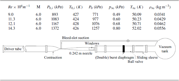


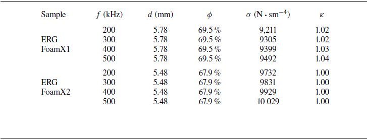


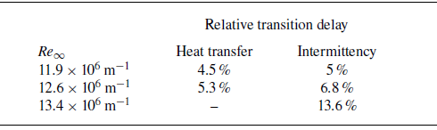


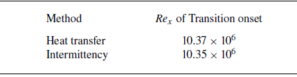


 Open access

