


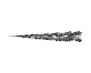



1. Introduction
This paper is a direct development from experimental and computational work that has already been reported in this journal (D'Ovidio & Coats (Reference D'Ovidio and Coats2013), McMullan, Gao & Coats (Reference Mcmullan, Gao and Coats2015) – hereinafter referred to as Part 1 and Part 2, respectively) and, to avoid repetition, readers are referred to those previous papers for more detailed reviews of the relevant background literature. The introductory discussion given here will instead return to the fundamental fluid-dynamic questions that have motivated all of this work, review the significant findings of Parts 1 and 2 in relation to these questions and explain how they are extended in this third paper.
The classical understanding of turbulence as random fluctuation about some time- or ensemble-averaged mean flow has its origins in the work of Reynolds (Reference Reynolds1895), who saw that an analogy can be made between such turbulent motions and the random motions of individual molecules. Provided that the scales of the individual fluctuations are small in relation to the thickness of any region of mean shear, the Reynolds stresses which quantify the fluctuations in the rate of transport of momentum within the flow then become quasi-physical quantities in their own right, their values reflecting empirically the effective local scale or intensity of the fluctuations. It therefore came as a severe challenge to classical turbulence theory when, in some turbulent shear flows, hot-wire anemometry showed individual fluctuations to be correlated over large intervals of space and time and even to display some degree of periodicity. Then, fifty years ago, flow visualisations unexpectedly showed high-Reynolds-number mixing layers with apparently normal mean profiles and growth rates to consist of processions of coherent vortex-like structures which occupied and effectively defined the full thickness of the region of turbulent shear (Brown & Roshko Reference Brown and Roshko1974). This stimulated two decades of intensive research on the plane mixing layer in the course of which a completely new model of its dynamics emerged and gained widespread acceptance.
The essential features of this model were reiterated relatively recently by Brown and Roshko as part of a wider-ranging review of the progress that had been made in turbulence research during the previous half-century (Brown & Roshko Reference Brown and Roshko2012). They can be summarised as follows:
(i) As in Taylor's theory, it is the spanwise vorticity within the flow that effects the transport of momentum in the cross-stream direction. However, that vorticity does not remain stably distributed within a continuous mass of rotational fluid. Instead, the growth of the layer involves a stepwise spontaneous concentration of the spanwise vorticity under the action of its own induction in accordance with the Biot–Savart relation. As was first proposed by Winant & Browand (Reference Winant and Browand1974), this begins with a random excitation of the Kelvin–Helmholtz instability of the layer's inflected velocity profile, the resultant quasi-periodic concentrations of vorticity subsequently amalgamating in pairs. These pairings are the products of sequential excitations of the sub-harmonics of the original Kelvin–Helmholtz mode. The growth of the layer is thus essentially a two-dimensional process which can be analysed without any direct involvement of energy considerations.
(ii) As the vorticity becomes concentrated within discrete vortex structures, tongues of irrotational fluid are drawn into the layer from the free streams and stagnate against each other to produce saddle-flow patterns in the spaces between the vortices (figure 1a). A consequence of this large-scale organisation is that the fluids entrained from the free streams eventually become mixed together in the vortex structures in a ratio that reflects the relative strengths of the entrainments from the two sides of the layer. This differs from the pattern of mixing in the classical turbulent mixing layer where the mean composition of the mixed fluid changes progressively from one side of the layer to the other.
(iii) The main effect of increasing Reynolds number, seen when a critical threshold (the ‘mixing transition’) is crossed, is a step increase in the amount of molecular-scale mixing within the layer. The small-scale turbulence that effects the additional mixing does not, as in a classical turbulent shear flow, take its energy directly from the mean shearing motion but is generated primarily at the interface between the tongues of entrained irrotational fluid by the straining of ‘streamwise’ vorticity there (i.e. of vorticity with components orthogonal to its original spanwise orientation) and subsequently transported into the cores of the vortex structures. Secondary streamwise vortices are formed in these interfaces upstream of the mixing transition as a result of localised tilting and subsequent stretching of the spanwise vortex lines and are assumed to survive the pairing interactions undergone by the primary spanwise vortices. It has been suggested that these secondary vortices may form a continuous thread of streamwise vorticity which winds forwards and backwards along the stretched interfaces (‘braids’) and around the cores of the spanwise vortex structures, as shown schematically in figure 1(b). Although not mentioned in the Brown & Roshko (Reference Brown and Roshko2012) review, there is experimental evidence that, in some circumstances at least, the spacing of the streamwise vortices doubles with each pairing of the spanwise ones (Huang & Ho Reference Huang and Ho1990; Bell & Mehta Reference Bell and Mehta1992). This finding has led to the suggestion that simultaneous quasi-periodic instability-driven doublings of both the streamwise and spanwise length scales constitute the mechanism by which the organised turbulent mixing layer grows in its fully developed self-similar state.
A question left completely unresolved by all this research was that of the relationship of such ‘organised’ turbulent mixing layers to the completely random mixing layer of classical turbulence theory. Mixing layers are notoriously sensitive to the initial conditions from which they develop and it has often been argued that, where large-scale organisation is present, it is a legacy of the initial conditions and will disappear eventually as the flow becomes fully developed. An alternative suggestion is that mixing layers never ‘forget’ their initial conditions entirely but relax towards an asymptotic state which is a function of both the free-stream and initial conditions (George Reference George, Arndt and George1989).
(a) Schematic representation of primary flow pattern and (b) hypothetical arrangement of secondary streamwise vortex lines (after Bernal & Roshko Reference Bernal and Roshko1986) in organised mixing layer.

The wind-tunnel experiments reported in Part 1 were undertaken to examine in more detail some earlier findings by Pedley (Reference Pedley1990) which appeared to contradict certain aspects of the two-dimensional instability-driven mixing-layer growth model outlined above. These more extensive and sophisticated experiments confirmed Pedley's finding that, at the mixing transition, there was not just a step increase in the amount of molecular-scale mixing within the developing mixing layer but also a change in the pattern of the large-scale motions. Before the transition the growth of the layer occurred essentially by vortex pairings, as had been proposed by Winant & Browand (Reference Winant and Browand1974), each pairing interaction drawing irrotational fluid into the layer and producing a step increase in its thickness. Beyond the transition, in contrast, the spanwise vortex structures all grew continuously at a constant rate. Interactions still occurred between neighbouring structures at intervals but they served merely to reduce the number of structures present so that their average spacing increased in proportion to their scale and the continuous growth of the structures that remained could continue unimpeded. The interactions thus occurred as a consequence of the growth but themselves contributed nothing to it. In most of these interactions both of the participating structures broke down, leaving a length of turbulent flow within which a new vortex structure would subsequently form and then grow continuously at the same rate as all the others. Occasionally a vortex structure would find itself closely confined between both of its immediate neighbours. In these circumstances the confined structure would cease growing and be fed upon by its growing neighbours. These latter were the sacrificial and ‘tearing’ interactions that had been identified earlier by Damms & Küchemann (Reference Damms and Küchemann1974) and Hernan & Jimenez (Reference Hernan and Jimenez1982). All of these features – the change in the pattern of interaction and growth at the mixing transition, the continuous constant-rate spanwise-averaged growth undergone by the individual vortex structures in the post-transition flow and the different types of destructive interaction the structures underwent there – were successfully replicated in the large-eddy simulations reported in Part 2.
As discussed in Parts 1 and 2, the continuous constant-rate growth undergone by the individual vortex structures in the post-transition flow is a feature of particular dynamic significance because it indicates that these structures are not, as has been so widely supposed, simple two-dimensional vortices containing turbulence of a much smaller scale. Rather they are the largest in the equilibrium three-dimensional cascade of eddy scales shown by hot-wire spectra to be active in the post-transition flow, continuously extracting energy from the mean shearing motion and passing it on to the smaller-scale motions. This in turn implies that the dynamics of the organised turbulent mixing layer differ fundamentally from those assumed in the two-dimensional instability-driven model outlined above in which the secondary streamwise vortices (figure 1b) responsible for the production of the small-scale turbulence ride more or less passively on the primary spanwise vortices. The stability of the continuously growing spanwise vortex structures seems to instead involve some kind of balance between the rate at which they acquire energy by the addition of fluid from the free streams and the rate at which that energy is passed down to the smaller scales. The possibility of such a balance is likely to be specific to the particular conditions of self-similarity that distinguish the spatially growing mixing layer from other types of turbulent shear flow.
The other finding of Pedley that was confirmed by the experiments reported in Part 1 was that the mixing layer is not always organised in this way. Periods in which the flow was organised into processions of spanwise-coherent vortex structures often alternated with periods in which the turbulent part of the layer resembled a classical turbulent shear flow. (A similar finding had been reported also by Karasso & Mungal Reference Karasso and Mungal1996.) It was observed moreover that, during the periods in which the large-scale organisation was absent, the layer grew at a slower rate and took up a different orientation relative to the fixed walls of the test section. The latter observation was particularly significant because it indicated a change in the ratio of the entrainment from the two free streams. It may be supposed that much of the well-documented variability in the mixing-layer growth rates measured in different laboratories (Brown & Roshko Reference Brown and Roshko1974) is attributable to the existence of these two different self-similar flow states for the same free-stream conditions. Quite apart from its theoretical significance, this bimodal behaviour is of obvious practical interest in connection with a wide range of engineering applications in which flows with thin boundary layers separate from solid surfaces, including particularly those involving combustion (Coats Reference Coats1996). There is renewed interest in such applications at the present time in connection with the urgent need to move away from conventional fossil-fuel-based combustion technologies.
The hypothesis tested in this paper is that the bimodality observed experimentally can be plausibly rationalised as a spontaneous switching, in response to small changes in the initial conditions, between two different self-similar turbulent flow states characterised by different balances of mass, momentum and energy. In one of these flow states the traditional Reynolds decomposition of the flow variables into their local first and second moments remains appropriate because the fluctuations are essentially random and relatively small in scale. In the other the eddies which effect most of the entrainment are ‘coherent’ in the sense that they are self-preserving, extend across the entire thickness of the region of mean shear and have a preferred orientation that is orthogonal to the mean shear. In this latter situation the individual fluid particles are no longer streaming independently, on average, along near-parallel mean streamlines and the dynamics of the spatial growth can be analysed only on an integral basis. Large-eddy simulations are first presented in which, with suitable manipulation of the initial conditions, one of the two-stream mixing layers studied experimentally in Part 1 and its single-stream counterpart (i.e. an otherwise identical flow in which the stream with the higher velocity entrains from a stagnant environment) have been simulated in both their classical and organised turbulent states. The simulation results for both flow states are then analysed dynamically on a model-free integral basis, showing clearly the differences in the mass, momentum and energy balances involved.
Section 2 of the paper describes the wind-tunnel experiment being replicated and outlines the simulation methods employed while § 3 summarises the findings of the numerous preliminary simulations that were performed in order to examine the sensitivity of the simulated flows to the use of different inflow and other boundary conditions. It was on the basis of these findings that the four cases selected for more detailed study were chosen. The results from these four simulations are then presented and compared in § 4 before being analysed theoretically in § 5. A summary of the main conclusions is given in § 6.
2. Wind-tunnel experiment replicated and simulation methods employed
The experiment chosen as the basis for all of the simulations presented here was the one labelled in Part 2 as HW10. As detailed in Part 1, two parallel streams of air supplied from a bank of high-pressure storage tanks had been smoothed, accelerated to the velocities u 1,0 = 32.0 m s−1 and u 2,0 = 12.9 m s−1 in convergent nozzles and brought together at the sharp trailing edge of a finely tapered splitter plate. Thus the Reynolds number per unit length applicable to this mixing layer was  $({u_{1,0}} - {u_{2,0}})/\nu = 1.3 \times {10^6}\;{\textrm{m}^{ - 1}}$, where ν is the kinematic viscosity of the fluid. The boundary layers on the higher- and lower-velocity sides of the splitter plate were both laminar at the point of separation with momentum thicknesses θ 1 = 1.1 × 10⁻⁴ m and θ 2 ∼ 2.0 × 10⁻⁴ m, respectively, and the root-mean-square (r.m.s.) intensities of the residual broad-band velocity fluctuations in the free streams discharged from the nozzles were ≤0.5 %. The mixing transition occurred approximately 0.075 m from the trailing edge of the splitter plate. The angle of the test-section wall bounding the lower-velocity stream had been adjusted once the flow was established to remove the positive streamwise pressure gradient which would otherwise have been present within the test section.
This particular experiment was chosen for further study because it was the one which best combined a relatively low value (0.43) of the velocity-ratio parameter  $R = ({u_1} - {u_2})/({u_1} + {u_2})$ with a good length of self-similar post-transition flow. To represent the limiting single-stream R = 1 case (one it had not been attempted to simulate in Part 2) comparative simulations have also been performed for an otherwise identical flow in which the higher-velocity stream was discharged with the same boundary-layer thickness and free-stream fluctuation intensity into a stagnant environment. The experiments reported in Part 1 had actually included some on single-stream mixing layers of different Reynolds numbers but, for the purposes of these simulations, it was considered desirable to retain exactly the same velocity and other inflow conditions for the moving stream. The Reynolds number per unit length applicable to this second mixing-layer flow was 2.2 × 10⁶ m−1.
In most respects the simulation methodology followed closely that which had been successfully used to replicate the same experimental flow in Part 2 but employed a differently constructed multigrid solver to permit the use of a wider range of boundary conditions. The transport equations were discretised and filtered spatially on a finite-volume basis as described in Part 2, the Wall-adapting Local Eddy-viscosity (WALE) model (Nicoud & Ducros Reference Nicoud and Ducros1999) being again used to provide an energy sink of approximately the correct magnitude for the cascading eddying motions resolved by the filter. This model has the considerable attraction that the sub-grid-scale eddy viscosity is zero in laminar shear flow so that, with a sufficiently fine grid, the developing unsteady motions in the pre-transition part of the mixing layer can be simulated with good accuracy. An earlier study (McMullan, Gao & Coats Reference Mcmullan, Gao and Coats2009) had shown that, in the type of flow of interest here, there was no significant backscatter from the unresolved to the resolved scales (Piomelli et al. Reference Piomelli, Cabot, Moin and Lee1991) so that the use of a computationally more expensive two-filter model was not justified.
Simulations of free turbulent shear flows performed with adequate resolution using the WALE model are relatively insensitive to the value of the model constant CW because the rate at which energy is extracted from the mean shearing motion and passed down to the dissipation scale is effectively determined by the rotations and straining interactions of the eddies resolved by the filter. Excessive damping can occur, however, if too high a value is used in simulations of flows containing wall boundary layers. To allow these new simulations to include studies of the effects of using non-slip walls as boundaries CW was therefore reduced from the value of 0.56 used in the earlier work to 0.325 – what has now become the standard value for use in such situations. As was shown in Part 2, variations over this range in the value of CW had no significant effect on the development of the mixing layer itself.
As before, a conserved scalar was introduced to label the fluid entrained into the mixing layer from the faster stream, a Schmidt number of 0.74 being applied to the sub-grid-scale diffusion. As with any large-eddy approach, the simulations were unable to quantify the mixing of the two fluids at the molecular scale but this was unimportant in the present context because the eddying and other induced motions that effected the entrainment and cross-stream transport in these turbulent flows were fully resolved by the filter. The filtered equations were solved iteratively with second-order spatial and temporal accuracy, a pressure correction being applied to maintain continuity of the fluid at each time step. Central differencing was used for the convective terms in the momentum equations and an implicit method for the time advancement.
In the simulations reported in Part 2, where the primary objective had been to produce time-resolved spanwise-averaged visualisations that could be compared with those made experimentally, approximately self-similar conditions had been created through the use of a computational domain of large cross-stream extent. Here, where the objectives included extension of the simulations to a higher value of R and – most critically – the production of conditions that were sufficiently self-similar to allow accurate determination of the relevant entrainment velocities and pressures, a different strategy was adopted. A domain of similar cross-stream extent to that of the wind tunnel's test section was employed, uniform free-stream conditions being created in the part of the domain containing the fully turbulent mixing layer by introducing a suitably profiled inflow through the cross-stream boundary on the low-velocity side (figure 2a).
(a) Computational domain and co-ordinate system. (b) Velocity profiles imposed at cross-stream inlet.

Because the pre- and post-transition parts of the organised mixing layer entrain at different rates, the forms of the velocity profiles imposed at the cross-stream inlet were as shown in figure 2(b). Both the streamwise component u and the cross-stream component v were ramped linearly in the pre-transition part of the flow (0 < x < xt) from their known values at x = 0 to whatever constant values were found by trial and error to give the closest approximation to self-similar flow at x > xt. The adjustments were made iteratively, the simulation being continued between adjustments for as long as was necessary for the fluctuation statistics to restabilise. To minimise the effects of the domain's finite length and prevent reverse flow through the outlet an exit section of variable length was introduced downstream of the main part of the domain. The conditions produced in this way provided a much closer approximation to self-similarity than was achieved in either the earlier simulations or the wind-tunnel experiments where the setting of the wall angle had taken no account of the differing entrainment appetites of the pre- and post-transition parts of the mixing layer. A further and more serious problem in the experiments had been that they often included periods of both organised and classical turbulent flow. Consequently, as was demonstrated and discussed in Part 1, the wall angles set will not have reflected the entrainment appetite of either turbulent flow state very accurately.
As in the original wind-tunnel experiment the span of the flow was 0.1 m. As was shown in Part 2, this was more than sufficient for the avoidance of spanwise confinement effects on the larger turbulent scales and the spatial growth rate of the mixing layer. Except where otherwise discussed, periodic boundary conditions were imposed at the ends of the span. The length of the main part of the computational domain was set at 0.3 m (nearly 3000θ 1) while its cross-stream extent was chosen to facilitate the most accurate setting of the required self-similar conditions. If the cross-stream boundaries were placed too close to the edges of the mixing layer then the flow disruptions associated with occasional interactions between the turbulent mixing layer and the domain boundary contaminated the fluctuation statistics. If the boundary on the lower-velocity side was too far away then it was no longer possible to profile the inflow through it to reflect the different entrainment appetites of the pre- and post-transition parts of the layer. The placements finally chosen were arrived at following trial simulations with domains of different dimensions. For the two-stream simulations these boundaries were placed at y = +0.035 and −0.045 m. For the single-stream simulations they were moved out to y = +0.05 and −0.1 m.
A mild boundary condition was applied at the domain outlet, this functioning merely to scale the velocities normal to the outlet so that the continuity of the fluid within the domain was maintained. Because the flow was treated as incompressible no acoustic waves were reflected at this boundary but the passage through it of concentrations of spanwise vorticity inevitably generated short-wavelength upstream-propagating numerical waves (Buell & Huerre Reference Buell and Huerre1988). To minimise their effect on the potentially susceptible pre-transition part of the flow the static pressure was fixed at mid-span at the location representing the trailing edge of the splitter plate, i.e. at the origin of the co-ordinate system shown in figure 2(a). With the pressure and velocity both specified at this inlet boundary location the numerical waves were progressively damped as they propagated upstream and were of near-zero amplitude in the initial part of the flow. The consequent variations of pressure at the outlet plane had no perceptible effect on the convection, growth and interactions of the turbulent vortex structures in the main part of the domain.
Hexahedral grids of between 35 and 42 million cells were employed in the definitive simulations, providing a similar spatial resolution to that in the simulations reported in Part 2. The grid was finest, with spacings Δx = 0.00015 m and Δy = 0.00004 m, at the trailing edge of the splitter plate and gradually expanded in both directions. These spacings resolved both the boundary layer separating from the higher-velocity side of the splitter plate and the wavelength of the fundamental Kelvin–Helmholtz mode with some 20 cells. The span of the domain was resolved with the uniform spacing Δz = 0.0006 m. To ensure adequate temporal resolution fixed time steps of 2 × 10⁻⁶ and 1.4 × 10⁻⁶ s were used in the two- and single-stream simulations respectively, giving cell Courant numbers <1 throughout the domain.
3. Effects of different inflow and other boundary conditions
A great many preliminary simulations were performed, mostly in smaller domains and in many cases with greater spatial and temporal resolution, to investigate systematically the effects of different inflow and other boundary conditions on the development of the two flows selected for study. Space limitations prevent any detailed presentation of the results here but, because of their direct relevance to the design of the full-scale simulations presented in § 4 as well as to the broader objectives of this research, a brief summary will be given of the principal findings.
In the simulations reported in Part 2 the low-level residual broad-band fluctuations that had been present in the inflows to the original wind-tunnel experiments were represented by introducing a spectrum of random uncorrelated fluctuations (effectively an injection of high-amplitude numerical noise) into the three components of the inflow velocity. With an r.m.s. fluctuation intensity equal to 0.5 % of the free-stream velocity this was sufficient to trigger the fundamental Kelvin–Helmholtz instability into rapid growth, leading to the development of an organised mixing layer in which the mixing transition occurred at a similar distance from the splitter plate to that which had been observed experimentally. This inflow noise was dissipated within the first few rows of grid cells, however, and had little or no direct effect on the flow further downstream. In these new simulations pseudo-physical inflow fluctuations were synthesised by the well-established method of summing a set of Fourier harmonics in such a way as to produce a divergence-free vector field in the form of small-amplitude three-dimensional wave motions (Kraichnan Reference Kraichnan1970; Smirnov, Shi & Celik Reference Smirnov, Shi and Celik2001). A set of 100 harmonics was used, spanning the range of wavenumbers defined by the dimensions of the inlet. As well as providing a better representation of the fluctuations remaining in the smoothed and accelerated inflows of the original wind-tunnel experiment, these coherent motions persisted within the free streams and proved much more effective in triggering the growth of three-dimensional instabilities in the developing mixing layer, even when of very small amplitude.
With inflow fluctuation intensities of up to 0.3–0.35 % of the free-stream velocity such fluctuations had the effect of triggering the fundamental Kelvin–Helmholtz instability into rapid growth, resulting again in the development of an organised turbulent mixing layer. However, there was also a partial loss of two-dimensionality in the rolled-up pre-transition flow. As seen in figure 3(a), individual vortices did not remain straight over the whole span of the flow but interacted helically with their neighbours and became linked with each other by streamwise-oriented vortices. This type of flow development has been studied experimentally by Chandrsuda et al. (Reference Chandrsuda, Mehta, Weir and Bradshaw1978) and Browand & Troutt (Reference Browand and Troutt1985) and seen also in the direct numerical and large-eddy simulations performed by Comte, Lesieur & Fouillet (Reference Comte, Lesieur, Fouillet, Moffatt and Tsinober1989) and Comte, Silvestrini & Bégou (Reference Comte, Silvestrini and Bégou1998).
Simultaneous perspective and spanwise views of iso-vorticity surfaces in initial part of mixing layer. In all views the y axis is vertical on the page and the flow direction from left to right. Light and dark areas on plotted iso-surfaces are regions in which the x component of vorticity is positive and negative respectively. Panels (a) and (b) show two-stream flow with random inflow fluctuations of intensity 0.1 %, ω = 1.5 × 10⁴ s−1 (perspective view) and 103 s−1 (spanwise view). Panels (c) and (d) show two-stream flow with random inflow fluctuations of intensity 0.5 %, ω = 2.5 × 10⁴ s−1 (perspective view) and 103 s−1 (spanwise view). Panels (e) and ( f) show single-stream flow with spanwise inflow sinuation of wavelength 0.003 m and r.m.s. amplitude 0.005u 1,0, ω = 2.5 × 10⁴ s−1.

At fluctuation intensities higher than 0.3–0.35 % there was a complete change in the pattern of flow development. Here the development of three-dimensionality (apparently associated with the growth of oblique instability modes rather than modes that were secondary to the fundamental Kelvin–Helmholtz instability) overtook the initial roll-up and the vortex sheet shed from the splitter plate broke down into a lattice of randomly oriented vortex tubes with little or no spanwise coherence (figure 3c). The outcome was a classical free turbulent shear flow in which there was a convoluted interface between rotational and irrotational fluid at the edges of the mixing layer but little or no penetration of irrotational fluid into its central region (figure 3d).
These results suggest that similar small variations in the inflow fluctuation intensity had been responsible for the observed switching between the organised and classical flow types in the experiments reported in Part 1. It is known that there had been small variations in the intensity of the residual inflow fluctuations within this range of values, both within and between individual experiments. The causes of these variations may have included transient aerodynamic resonances within the blow-down air supply systems at particular flow conditions and/or compaction of semi-rigid porous packings used within the flow smoothing process.
Residual inflow fluctuations are not the only source of three-dimensionality in nominally plane mixing layers, however. As was discussed in § 1, regular arrays of secondary counter-rotating streamwise vortex pairs at fixed spanwise locations have often been found, superimposed on the primary spanwise vortices, in mixing layers developing from laminar initial conditions. In some cases at least the fixed locations of such vortex pairs have been linked to the presence of imperfections in the screens used to smooth the experimental inflows. It seems that the presence of a vestigial wake or other defect at a particular spanwise location can excite the translative instability of the rolled-up flow (Pierrehumbert & Widnall Reference Pierrehumbert and Widnall1982) which then propagates itself laterally across the span of the flow (Lasheras, Cho & Maxworthy Reference Lasheras, Cho and Maxworthy1986; Nygaard & Glezer Reference Nygaard and Glezer1991). Straining of the streamwise vorticity in the braids connecting the spanwise vortices during the pairings undergone by the latter then excites a braid instability which causes the streamwise vorticity to become concentrated within a stationary array of counter-rotating streamwise-oriented vortices (Lin & Corcos Reference Lin and Corcos1984; Neu Reference Neu1984).
To accurately reproduce the spanwise propagation of the translative instability from a single inflow defect would require direct numerical rather than large-eddy simulation. However, with sufficient spatial and temporal resolution, the excitation of the translative instability and the subsequent formation of the secondary streamwise vortices were successfully captured in these preliminary simulations in response to spanwise sinuations in the inflow velocity with r.m.s. levels smaller than 0.5 % of its average value (figure 3e). An unexpected and significant finding of these particular studies was that in no case did the regular arrays of streamwise vortices formed in the pre-transition flow survive the mixing transition. As will be discussed in § 4, both single and paired streamwise vortices were to be found in the post-transition mixing layer but they were not, in general, continuous with any formed upstream of the transition location. This suggests that continuous threads of streamwise vorticity of the type represented schematically in figure 1(b) are specifically a feature of the pre-transition flow.
In this connection there is an important distinction to be made between the streamwise vortices formed in the separated flow, as described above, and the preformed arrays of streamwise vortices that were introduced diagnostically as part of the inflow in the large-eddy simulations of McMullan & Garrett (Reference Mcmullan and Garrett2016a,Reference Mcmullan and Garrettb). Those vortices were generated in a ‘precursor’ flat-plate boundary-layer simulation by means of a recursive procedure with two special features:- (i) the prescribed profiles for the velocity fluctuations in the three co-ordinate directions were strongly anisotropic, promoting the creation of streamwise vorticity; (ii) the statistical homogeneity imposed in the spanwise direction was such that it was only the spanwise averages of the first and second velocity moments that were constrained to match the prescribed profiles, allowing the streamwise vorticity to become concentrated in a parallel array of counter-rotating vortices. The precursor simulation thus functioned somewhat like a row of vortex generators mounted on the splitter plate. In this situation the continuous counter-rotating threads of concentrated streamwise vorticity shed from the splitter plate had the effect of delaying or preventing altogether the transition of the mixing layer to its organised fully turbulent state, the layer continuing to grow by a process of sequential vortex pairing.
Returning to the present simulations, it was found that, even without excitation of the translative instability, the presence of any small spanwise non-uniformity in the inflow tended to inhibit the development of more randomised three-dimensionality. In the rolled-up flow a single small vestigial wake was sufficient to act as a fixed node, reducing the effective span of the flow and thus preventing excitation of the lower-wavenumber helical pairing modes. It thus seems that whether the pre-transition flow develops as in figure 1(b) or figure 3(a), or as something between the two, depends on features specific to individual realisations that it is difficult to either control in real mixing layers or represent generically in simulations. It is important to note, however, that these differences in the pattern of the pre-transition development had no obvious effect on the character or growth rate of the post-transition flow – the part of the organised mixing layer of interest in this study.
Attention was also given in the preliminary simulations to the influence, as sources of three-dimensionality, of the boundary conditions applied at the ends of the span. Replacement of the periodic boundaries with non-slip walls representative of those present in the original experiment showed that the drag of the wall boundary layers imparted a twisting moment to the ends of the spanwise vortices so that their pairings had a strongly helical character. It was also found that, during the pairings, rotational boundary-layer fluid was sucked away from the walls and along the axis about which the pairing vortices were rotating. In simulations containing these non-slip walls it was usually the twisting of the vortex ends during a pairing that initiated the mixing transition.
4. Simulation results
In the light of the results of the preliminary simulations summarised in § 3 and following comparisons with spark-shadowgraph plan-view visualisations of the original experimental flows (e.g. that reproduced in figure 5 of Part 1), four test cases were chosen for more detailed study. To simulate both the single- and two-stream flows in their organised states random fluctuations with intensities of 0.15 % were introduced into the inflows through inlets 1 and 2 (figure 2a). This was the intensity level necessary for completion of the mixing transition (in the sense that a spanwise-coherent fully turbulent flow was established across the full span of the domain) at the experimentally observed distance of about 0.075 m (700θ 1) from the trailing edge of the splitter plate. Fluctuations were not applied to the boundary layers separating from the two sides of the splitter plate because these were of sub-critical Reynolds number and, in the original experiments, viscous forces and the strong negative pressure gradient associated with the acceleration of the inflows will have effectively damped out any fluctuations within them. To simulate the two flows in their classical turbulent states the inflow fluctuation intensities were increased to 0.5 %, the highest level recorded in the experiments. Periodic boundaries were retained at the ends of the span because the local flow separations from non-slip walls induced by the large-scale motions would have compromised significantly the creation of the desired self-similar conditions for the organised post-transition flow.
As detailed in § 2, the magnitudes of the inflow velocities u 2 and v 2 through the cross-stream inlet (figure 2) needed to produce self-similar conditions for the fully turbulent part of the mixing layer were established for each of the four test cases by a lengthy process of systematic iteration. This was achieved for v 2 with an estimated precision of ±2 % in the cases of the two-stream flows and ±5 % in those of the single-stream ones, the magnitude of any residual variation in the value of u 1 in the notionally self-similar part of the flow being always less than 0.5 %. These v 2 values are listed as ranges of uncertainty in tables 1 and 2 together with the corresponding values for the streamwise velocities u 1 and u 2 (which were measurably different from the inlet values u 1,0 and u 2,0) and certain other characteristics of the self-similar flow which will be discussed later. The mean static pressure difference across the mixing layer, p 1–p 2, could be determined with reasonable precision for the two-stream flows but only very approximately for the single-stream ones because of the practical impossibility of completely eliminating induced streamwise motions (and consequent streamwise pressure variations) in the irrotational fluid discharged from the cross-stream inlet. Once these flow conditions had been established the simulations were continued for as long as was necessary for the fluctuation statistics to stabilise.
Similarity parameters for test cases involving classical turbulent flow.

Similarity parameters for test cases involving organised turbulent flow.

As in Part 2, the mean velocity and scalar profiles presented will be of time-mean values that have been averaged also over the span of the domain (denoted as  ${\langle \bar{u}\rangle _{z,t}}$, etc.). All of the results and analyses are presented in dimensional form because:-
(i) as was discussed in § 1 and will be demonstrated in § 5, different analytical frameworks are required for the mixing layer in its organised and classical states;
(ii) as will be shown, some of the features of the organised post-transition layer are Reynolds-number-dependent.
As was noted in § 3, the streamwise vortices present in the organised post-transition mixing layer were not continuous with any formed in the pre-transition flow and a close study was therefore made of their genesis with the aid of visualisations such as that shown in figure 4(a). As was shown in Parts 1 and 2 and summarised in § 1, pairs of spanwise vortex structures break down at intervals when their continuous growth has reached the point at which the saddle-flow pattern between them can no longer be sustained. Now the cores of the structures are formed of bundles of vortex tubes with a preferential spanwise orientation, each breakdown of two neighbouring structures leaving a three-dimensional tangle of such tubes. As a single new structure forms to replace the two that have broken down the vortex tubes that are to constitute its core become oriented in the spanwise direction once more while those more remote from the axis of the roll-up become stretched in the braids linking the new spanwise vortex structure to its neighbours. This appears to be the process by which the braids are refreshed at intervals with concentrations of streamwise vorticity, allowing the continuous energy cascade within the growing structures to be sustained. Pairs of counter-rotating streamwise vortices of smaller scale may also be formed within the braids by local excitations of the braid instability (Lin & Corcos Reference Lin and Corcos1984; Neu Reference Neu1984) but this is incidental. The spanwise distribution of the vorticity within both the spanwise vortex structures and their linking braids is in consequence very irregular. In the light of what is to be seen in visualisations of this kind, the suggestion made in Part 2 that significant vorticity of the opposite hand to that of the mean shear might be introduced locally by the bending of stretched streamwise vortices around the cores of the spanwise vortex structures (cf. figure 1b) must now be rejected.
Instantaneous visualisations of organised post-transition flow: (a) ω = 104 s−1 iso-vorticity surfaces (plan view with direction of flow from left to right) in two-stream mixing layer, shaded as in figure 3 and showing, near the middle of the visualised flow length, a region of chaotic flow resulting from the breakdown of neighbouring vortex structures; (b) y–z cross-sections through braid, R = 0.43, x = 0.118 m; (c) y–z cross-section through core of spanwise vortex structure, R = 0.43, x = 0.128 m; (d) y–z cross-section through braid, R = 1, x = 0.136 m; (e) y–z cross-section through core of spanwise vortex structure, R = 1, x = 0.182 m. The three contour lines plotted in (b–e) are of ξ = 0.1, 0.5 and 0.9, the light shading is vorticity magnitude and the broken lines are the locations at which  ${\langle \bar{\xi }\rangle _{z,t}} = 0.01$ and 0.99.

Normalised spanwise-averaged spatial growth of simulated mixing layers in their (a) organised and (b) classical turbulent states. The reference line of gradient  ${\rm \pi}^{-1}$ is the growth rate given by (5.4).

The extent of this spanwise irregularity is evident from the representative instantaneous y–z cuts presented in figure 4(b–e). Figure 4(b) shows clearly the presence of some streamwise vortices of alternating hand in the braids of the two-stream flow. They are barely evident at all, however, in the corresponding cut of the single-stream flow (figure 4d). The significant difference here is that the Reynolds number, scaled on the thickness of the mixing layer and the velocity difference across it, is some four times greater and the thin semi-laminar braids of the two-stream flow have been replaced with thicker strained sheets of more fully turbulent fluid.
That this inherent large-scale spanwise irregularity and its sensitivity to Reynolds number complicate the determination of a dynamically meaningful spatial growth rate for the organised post-transition mixing layer is shown in figure 5(a). Here, an attempt has been made to plot a normalised spatial growth rate, which in the asymptotic limit is expected to be proportional to R, as a function of distance from a virtual origin at x 0 for both the single- and two-stream flows using four different measures of the local layer thickness. These are the momentum thickness
 \begin{equation}\theta (x) = \frac{{\int_{ - \infty }^\infty {({u_1} - {{\langle \bar{u}\rangle }_{z,t}})({{\langle \bar{u}\rangle }_{z,t}} - {u_2})\,\textrm{d}y} }}{{{{({u_1} - {u_2})}^2}}},\end{equation}
the vorticity thickness
 \begin{equation}{\delta _\omega }(x) = \frac{{{u_1} - {u_2}}}{{{{(\textrm{d}{{\langle \bar{u}\rangle }_{z,t}}/\textrm{d}y)}_{max}}}},\end{equation}
and two others based on the mass fraction ξ of the fluid entrained from the faster stream. These are the cross-stream distance between the points at which  ${\langle \bar{\xi }\rangle _{z,t}} = 0.01$ and 0.99 (denoted as δ 99) and that between the points at which
 ${\langle \bar{\xi }\rangle _{z,t}} = 0.00001$ and 0.99999 (denoted simply as δ). As can be seen from figure 4(b–e), δ 99 is likely to be of comparable magnitude to an experimental spanwise-integrated visual thickness.
 ${\langle \bar{\xi }\rangle _{z,t}} = 0.00001$ and 0.99999, on the other hand, approximated closely to the actual edges of the turbulent mixing layer, i.e. the locations at which the mean velocities, static pressures and scalar mass fractions all began to depart from their free-stream values. These locations could be determined with some precision with the level of free-stream uniformity and the spatial resolution available in these simulations. The significance of the reference line of gradient
 ${\rm \pi}^{-1}$ will be discussed in § 5.1. It is important to note that all of the simulation results presented in this and the subsequent figures were fully converged statistically. The minor wiggles evident in the streamwise plots – most obviously those of δ/R and δ 99/R – reflect the minor departures from perfect uniformity of the free streams.
All of the data plotted in figure 5(a) are for the post-transition flow in the range of x values 900θ 1 < x < 2700θ 1, a range within which self-similar growth might reasonably be expected (Bradshaw Reference Bradshaw1966). Unsurprisingly, the integral measure of thickness, θ, and that based on the velocity gradient in the centre of the mixing layer, δω, show something approximating more closely to self-similar growth than δ 99 and δ, both of which were very much more sensitive to local departures from perfect uniformity in the free streams. More significantly, all four measures of the layer's thickness show that the normalised growth rates for the (lower-Reynolds-number) two-stream flow were up to 30 % greater than those for the (higher-Reynolds-number) single-stream one. As shown by figure 4(b–e) this is because, at the lower Reynolds number, the thickness of the mixing layer, as measured on a time- and spanwise-averaged basis, included a greater proportion of completely unmixed and irrotational fluid indistinguishable from that external to the layer. Much of this was to be found in the tongues of entrained fluid which separated the cores of the vortex structures but, as figure 4(c,e) show, a lot more was located at the edges of the mixing layer where the turbulent cores of the vortex structures ‘nibbled’ directly at the free streams. Hot-wire measurements would have shown these two mixing layers as differing from each other in having not just different growth rates but also different turbulence intermittency levels.
This is in contrast with the situation in relation to the two classical turbulent mixing layers (figure 5b) where, with the same Reynolds-number difference between the single- and two-stream flows, their normalised self-similar growth rates are more nearly the same. (The residual differences between the plots for the two flows are not significant and can be attributed to the imperfect realisation of the desired self-similar conditions in the simulations.) Comparison between the two figures shows that the growth rates for the organised flow relax towards those for the classical flow as the Reynolds number is increased. These characteristics explain why, in the flow-visualisation experiments reported in Part 1, the growth rate was consistently observed to be greater when the flow was in its organised state.
The profiles of  ${\langle \bar{u}\rangle _{z,t}}$ and
 ${\langle \bar{\xi }\rangle _{z,t}}$ at different streamwise locations are plotted as functions of the non-dimensional co-ordinate
 $\eta = y/(x - {x_0})$ in figure 6. Those of
 ${\langle \bar{u}\rangle _{z,t}}$ are of the near-antisymmetric forms expected where the fluid is of uniform density, their shapes reflecting the relationships between θ, δω and δ seen in figure 5. Indicated for the two organised flows in figure 6(a,c) is the position on the profile at which
 ${\langle \bar{u}\rangle _{z,t}}$ was equal to
 $({u_1} + {u_2})/2$. This was the approximate location of the axis along which the entrained tongues of irrotational fluid stagnated against each other and the centres of rotation of the continuously growing vortex structures convected (Coles Reference Coles1985; Dimotakis Reference Dimotakis1986) and was close to the locations of both the maximum of
 $\textrm{d}{\langle \bar{u}\rangle _{z,t}}/\textrm{d}y$ and the minimum of
 ${\langle \bar{p}\rangle _{z,t}}$. In practice this location could be determined more accurately from the simulation results than that of the maximum of
 $\textrm{d}{\langle \bar{u}\rangle _{z,t}}/\textrm{d}y$ and its streamwise variation was extrapolated back to y = 0 to establish a dynamically meaningful virtual origin for each of the two organised mixing layers.
Similarity profiles of  ${\langle \bar{u}\rangle _{z,t}}$ and
 ${\langle \bar{\xi }\rangle _{z,t}}$: (a,b) organised flow, R = 0.43; (c,d) organised flow, R = 1; (e,f) classical flow, R = 0.43; (g,h) classical flow, R = 1. The vertical reference lines in (a–d) indicate the location of the axis along which the entrained tongues of irrotational fluid stagnated against each other.

More interesting differences are to be seen between the corresponding profiles of  ${\langle \bar{\xi }\rangle _{z,t}}$. Those for the two classical flows (figure 6 f,h) are near linear over the central part of the mixing layer, as predicted by classical turbulence theory, but become curved towards the edges of the layer because of the presence there of sizeable indentations in the interface between the entrained irrotational fluid and the rotational (turbulent) fluid that has already undergone some mixing. The profiles for the two organised flows (figure 6b,d) are significantly different, however, and show that the composition and distribution of the mixed fluid within the layer continued to change long after the dynamics of the spatial growth had attained approximate self-similarity. This is consistent with the experimental observations of Karasso & Mungal (Reference Karasso and Mungal1996), Slessor, Bond & Dimotakis (Reference Slessor, Bond and Dimotakis1998) and Meyer, Dutton & Lucht (Reference Meyer, Dutton and Lucht2006). The location of the axis along which the entrained inflows stagnated and the centres of rotation of the vortex structures convected is again indicated in these two figures. In both cases there is a very obvious flattening of the profile in the central part of the layer immediately downstream of the mixing transition, this feature becoming progressively less marked further downstream. In the case of the two-stream flow (figure 6b) there is also a significant fall with increasing x in the value of
 ${\langle \bar{\xi }\rangle _{z,t}}$ at the axis of stagnation.
Both of these features are reflected in figure 7(a,b), which presents the probability-density functions (pdfs) of ξ sampled at five different cross-stream and two different streamwise locations in the two-stream organised layer. As was noted in § 2, these pdfs do not take account of sub-grid-scale unmixedness but provide a level of spatial resolution that is perfectly adequate for study of the scalar transport in these gaseous flows. Marked in these figures is the value of η at which the entrained flows stagnated against each other and the centres of rotation of the vortex structures were located. It is seen that the values of  ${\langle \bar{\xi }\rangle _{z,t}}$ at this cross-stream location in figure 6(b) provide a good measure of the average composition of the mixed fluid within the vortex structures and that the reduction in the flattening of the profile of
 ${\langle \bar{\xi }\rangle _{z,t}}$ with increasing x reflects an increasing amount of mixing at more dispersed values of ξ. Figure 7(c) presents for comparison a representative set of pdfs for the two-stream classical layer. As expected, these are of the ‘marching’ type showing, at each cross-stream location, a random distribution of compositions about a mean value of ξ which falls continuously with decreasing η.
Mixture-fraction pdfs at z = 0 in R = 0.43 mixing layer: (a) organised flow, x = 0.15 m; (b) organised flow, x = 0.25 m; (c) classical flow, x = 0.25 m. The vertical reference lines in (a) and (b) indicate the location of the axis along which the entrained tongues of irrotational fluid stagnated against each other.

That the range of mixture fractions present within the organised mixing layer continues to increase for some distance downstream of the mixing transition has been discussed fairly extensively in the literature where it has been described as a switch from a ‘non-marching’ to a ‘tilted’ or ‘hybrid’ form of pdf. From consideration of the available empirical evidence, Karasso & Mungal (Reference Karasso and Mungal1996) proposed that this switch occurred when the ‘pairing parameter’ Rx/λ, where λ is the wavelength of the initial Kelvin–Helmholtz instability, attained a value of ∼22. Huang & Ho (Reference Huang and Ho1990) had earlier proposed that, in a mixing layer which grew by a sequence of vortex pairings, those pairings might be expected to occur at the locations at which this parameter attained the approximate values 4, 8, 16, etc., the mixing transition typically being triggered by the second such pairing. The logic of the proposal made by Karasso & Mungal was that the switch from the non-marching to the tilted form of pdf occurred with the first vortex pairing following the mixing transition. As was shown in Parts 1 and 2, vortex pairings of the pre-transition type do not actually occur downstream of the mixing transition, the turbulent vortex structures instead interacting destructively at intervals with the production of regions of temporarily chaotic turbulent shear flow. A better explanation for the change in the forms of the mixture-fraction pdfs at x > 2xt is therefore that this reflects the added contribution to the statistics of the intermittent local breakdowns in the large-scale organisation. If, following Huang & Ho, λ is evaluated as 29.4θ 1 then the pdfs presented in figure 7(a,b) will have corresponded to values of 19.9 and 33.2 for the pairing parameter, neatly bracketing the critical value proposed by Karasso & Mungal.
The fall with increasing x, in the case of the two-stream organised mixing layer, in the average value of ξ within the large structures (figure 7a,b) and in the resultant value of  ${\langle \bar{\xi }\rangle _{z,t}}$ at the axis of stagnation (figure 6b) appears to be an effect of the presence of the splitter-plate wake. Because the initial Kelvin–Helmholtz roll-up occurred on the higher-velocity side of the wake most of the fluid within the pre-transition mixing layer had originated in the faster stream. It was only downstream of the mixing transition that the layer entrained and grew in a quasi-self-similar way, the more nearly balanced entrainment of the two fluids progressively reducing the average value of ξ of the mixed fluid within the layer.
This is a feature of some importance because most of the published experimental research involving scalar measurements has, for practical reasons, been performed on two-stream mixing layers of modest length. In all of this work the assumption has been made that the average value of ξ at the measurement location was itself a measure of the ratio of the self-similar entrainments from the two sides of the layer. On the basis of scalar measurements made at R = 0.45 by Konrad (Reference Konrad1976), supplemented by kinematic arguments, Dimotakis (Reference Dimotakis1986) has proposed that the ratio of the volumetric entrainments from the two sides of uniform-density mixing layers is given by the relationship
 \begin{equation}{E_V} = 1 + 0.68R.\end{equation}
The present simulation results indicate that the asymptotic value of EV for the organised layer is actually somewhat lower than this, increasing from ∼1.2 at R = 0.43 to only ∼1.3 at R = 1.
The final features of the simulation results to which attention will be drawn concern the average shear stress acting across the fully turbulent mixing layer and the rate of energy dissipation within it. It was suggested in Part 2 that the flow adopts its organised state where the inflow and other conditions allow because this offers the ‘path of least resistance’ for progressive relief of the shear stress across the layer. That this is so is confirmed by the results presented in figure 8(a). Here, the principal component of the shear stress, averaged across the layer as
 \begin{equation}{\left\langle {\overline {{\tau_y}} } \right\rangle _{y,z,t}} = \frac{{\int_{{y_{0.00001}}}^{{y_{0.99999}}} {{{\left\langle {\overline {(\mu + {\mu_{SGS}})\dfrac{{\textrm{d}u}}{{\textrm{d}y}}} } \right\rangle }_{z,t}}\textrm{d}y} }}{{{y_{0.99999}} - {y_{0.00001}}}},\end{equation}
where μ and  $\mu_{SGS}$ are the molecular and (sub-grid-scale) eddy viscosities and y 0.00001 and y 0.99999 the cross-stream locations at which
 ${\langle \bar{\xi }\rangle _{z,t}} = 0.00001$ and 0.99999, is plotted with suitable normalisation as a function of distance from the virtual origin for all four test cases. Too much significance should not be given to the absolute values estimated in this way for the average shear stress acting across the layer because of the use of a sub-grid-scale model to represent the eddying motions unresolved by the filter. The same filter was used in all four simulations, however, and so the figure can be taken to accurately reflect the effects of the differing vorticity distributions in the four simulated flows. It is seen that the organisation of the mixing layer into a procession of roller-like spanwise vortex structures separated from each other by regions of near-potential flow does in fact reduce the shear stress against which work must be done by up to some 50 %.
Comparison of (a) normalised average shear stresses and (b) normalised energy dissipation rates within the organised and classical turbulent mixing layers.

That the flow organises itself in this way where the inflow and other conditions allow is a corollary of the second law of thermodynamics which requires that any macroscopic non-equilibrium system with time-invariant boundary conditions must approach its final equilibrium state by the path that minimises its internal rate of entropy production (Glansdorff & Prigogine Reference Glansdorff and Prigogine1964). In figure 8(b) the average rates of energy dissipation per unit volume of mixing-layer fluid
 \begin{equation}\rho {\langle \bar{\varepsilon }\rangle _{y,z,t}} = \frac{{\int_{{y_{0.00001}}}^{{y_{0.99999}}} {{{\left\langle {\overline {(\mu + {\mu_{SGS}}){\boldsymbol{S}^\textrm{2}}} } \right\rangle }_{z,t}}\textrm{d}y} }}{{{y_{0.99999}} - {y_{0.00001}}}},\end{equation}
where ρ is the fluid density and S2 represents the second invariant of the rate-of-strain tensor, are plotted on the same basis as the data in figure 8(a) showing directly this principle in action. It should be noted that the plots for the two organised flows in figure 8(b) show the same Reynolds-number dependence as was seen in figure 5(a). This is because the amount of irrotational fluid (within which there is no energy dissipation) swept along within the organised mixing layer decreases with increasing Reynolds number.
5. Theoretical analyses
5.1. Fundamental considerations
In text-book analyses of the classical turbulent mixing layer it is usual to concentrate on the exchange of just the streamwise momentum between the fluids entrained from the two sides of the layer and, in this context, it has often been found convenient to quantify the growth of the mixing layer in terms of its momentum thickness. Indeed, the balance of cross-stream momentum has usually been ignored altogether. As will be shown in § 5.3, in the case of the organised layer the balances of the cross-stream momentum and the associated stagnation energy are as important as that of the streamwise momentum. In order to be able to compare the dynamics of the self-similar spatial growth of the organised and classical layers in a meaningful way it is therefore necessary to establish also an analysis of the classical layer which similarly includes a proper balance of the cross-stream momentum. This will be the subject of § 5.2. A further complication, however, is that, as was shown in § 4, the organised layer (unlike its classical counterpart) contains a great deal of entrained irrotational fluid which, by definition, has yet to exchange any of its mass, momentum and energy with the rotational fluid within the layer. What is also required, therefore, is a measure of the growth rate which defines specifically the rate of increase in the mass of the rotational fluid within the layer.
Where the fluid is incompressible this growth rate can be defined kinematically by reference to the equiangular (logarithmic) spiral that was introduced, in a slightly different analytical context, in Part 2. Consider figure 9 which represents the situation in a temporally growing mixing layer formed between two counter-flowing free streams of speed u∞/2. Because the growth of the layer is self-similar the lengths of the straight lines OP and OQ increase at the constant rate dr/dt as fluid particles detach themselves from the free streams and begin to exchange momentum and energy. Because there is symmetry with respect to the x axis and no momentum is being created or destroyed by the exchange process, the net streamwise velocity with which fluid crosses the line POQ is zero. The two equiangular spirals issuing from the pole at point O are the virtual streaklines formed by the particles which, at successive instants of time, have entered the layer at the outwardly moving points P and Q. Now it is a property of the equiangular spiral that its length increases at a constant rate as it rotates. As will be shown, this figure therefore defines the unique rate at which the ‘rotational thickness’ of the layer can increase linearly if the essential continuity of the fluid is to be preserved.
Equiangular spirals defining temporal growth rate of region of self-similar simultaneous mass and momentum exchange between counter-flowing streams.

Although it was used in Part 2 to estimate the growth rate of the spanwise structures in the organised post-transition layer (a growth rate which can be taken to define that of the layer as a whole where the flow is in its organised state), this spiral transform should not be confused with the rolling-up of a vortex sheet. The spiral associated with the rolling-up of a vortex sheet is formed of streamlines, not streaklines, and it is not an equiangular one: its length increases continuously towards the centre of the rotation and, in the absence of viscous forces, becomes infinite at the pole. All that is being analysed here is the fundamental kinematic constraint imposed by the requirement for continuity on the rate of a linearly self-similar simultaneous exchange of mass and momentum in an incompressible fluid. This constraint necessarily applies in all such situations, irrespective of the details of the actual exchange process involved.
Now the essential feature of an equiangular spiral is that the radius r at any point along its length increases exponentially with that point's angle of rotation φ such that
 \begin{equation}\frac{r}{{{r_0}}} = \exp (c|\varphi - {\varphi _0}|),\end{equation}
where r 0 and φ 0 are the radius and angle of rotation of some other reference point on the spiral and c is a constant. Consequently, if one of these points is rotated through an angle of 2 ${\rm \pi}$ radians relative to the other,
 $r = {r_0}\exp (2{\rm \pi} c)$. It also follows that for both points to lie on the same line OP or OQ, so that the growth in the thickness of the mixing layer as well as in the length of the spiral is self-similar, c must be (2
 ${\rm \pi}$)−1, making
 $r = e{r_0}$and the ratio r/r 0 a constant.
Consider now the increases in the length l of each of the two spirals at the outwardly moving points P and Q. Because  $\textrm{d}l = r\,\textrm{d}\varphi$,
 \begin{equation}l - {l_0} = \int_{{\varphi _0}}^\varphi {r\,\textrm{d}\varphi } = 2{\rm \pi} (r - {r_0}),\end{equation}
from which dl/dr = 2 ${\rm \pi}$. But dl/dt at both P and Q is u∞/2 and consequently the temporal growth rate of the mixing layer's thickness is
 \begin{equation}2\frac{{\textrm{d}r}}{{\textrm{d}t}} = 2\frac{{\textrm{d}r}}{{\textrm{d}l}}\frac{{\textrm{d}l}}{{\textrm{d}t}} = \frac{{{u_\infty }}}{{2{\rm \pi} }}.\end{equation}
If the two counter-flowing streams are replaced with two streams moving in parallel with the velocities u 1 and u 2 (u 1 > u 2) then
 \begin{equation}2\frac{{\textrm{d}r}}{{\textrm{d}{\kern0.8pt}x}} = 2\frac{{\textrm{d}r}}{{\textrm{d}t}}\frac{{\textrm{d}t}}{{\textrm{d}{\kern0.8pt}x}} = \frac{{{u_1} - {u_2}}}{{2{\rm \pi} }}\frac{2}{{{u_1} + {u_2}}} = \frac{R}{{\rm \pi} }.\end{equation}
This equation defines, to a very close approximation, the rate of spatial growth of the thickness of the rotational fluid within any real self-similar mixing layer of uniform density. As already discussed, the temporal growth rate (5.3) is exact and fundamental. The spatial growth rate (5.4) will be in error when applied to a real flow only to the extent that streamwise momentum is not conserved overall in the growth process. In the real spatially growing mixing layer there will be a very small gain or loss of streamwise momentum as a result of the pressure differences associated with asymmetry of the entrainment from the two sides of the layer but this is negligible in relation to the magnitudes of the streamwise momentum fluxes involved and is conventionally ignored in all text-book analyses.
Figure 5(b) shows that, to within the precision with which δ was determined in the simulations, (5.4) is in perfect agreement with the simulation results for the two classical turbulent mixing layers – the two that contain little or no irrotational fluid within the region of mean shear. This is not the case for the two organised layers, however, and in figure 5(a) the ratio of δ/R to the reference thickness (x − x 0)/ ${\rm \pi}$ can be taken to provide a direct measure of the relative proportions of the irrotational and rotational fluid contained within the spanwise-averaged thickness δ. Figure 10 plots the resultant proportion of the irrotational fluid within the two organised layers as a function of the local Reynolds number Reδ = δ(u 1 − u 2)/ν. The trend discussed qualitatively in § 4 is very clear and continues to a Reynolds number of at least 2.5 × 10⁵. The apparent flattening of the curve at the highest values plotted is not significant and reflects a small influence of the increasing proximity of the exit boundary in the single-stream simulation.
Fraction of irrotational fluid within thickness of organised mixing layer vs. Reynolds number.

It may be noted that, in wind-tunnel experiments, Clemens & Mungal (Reference Clemens and Mungal1995) observed the large-scale organisation to persist to Reynolds numbers of roughly twice the highest value attained in these simulations before the compressibility effects associated with their use of high convective Mach numbers began to modify it significantly. More data would be required to know whether or not there is a limiting Reynolds number above which the layer cannot exist in its organised state. As was seen in figures 4(b) and 4(d), some of the decrease in the proportion of the fluid within the layer that is irrotational can be attributed to the thickening of the braids. However, the principal reason for the decrease appears to be simply that the spanwise non-uniformity of the organised layer decreases with increasing Reynolds number.
5.2. Dynamics of the classical turbulent mixing layer
The kinematically defined growth rate (5.4) will first be applied to the mass and momentum exchanges occurring in the two test cases involving classical turbulent mixing layers. The control volume OPQ in figure 11(a) represents unit length of the self-similar layer plotted in co-ordinates which spring from its virtual origin. Outside this volume is completely unmixed irrotational free-stream fluid in which the mean static pressure is uniform, the static pressures being different on the two sides of the layer. The faster stream, as in the simulations and the wind-tunnel experiments, is parallel to the x axis while the slower one has a resultant velocity which is at an angle to this axis. In the single-stream (R = 1) case u 2 is zero and this angle becomes 90°. All angles will be taken as positive when associated with anti-clockwise rotations.
Analytical frameworks for (a) classical and (b) organised turbulent mixing layer.

For continuity the entrainment into the control volume from the free streams must be equal to the outflow through the plane PQ. Consequently, if the control volume is taken to be of unit length in the x and z directions,
 \begin{equation}{u_1}\tan {\alpha _1} - {u_2}\tan {\alpha _2} + {v_2} = \int_{\tan {\alpha _2}}^{\tan {\alpha _1}} {\bar{u}(y)\,\textrm{d}y} ,\end{equation}
where the overbar denotes a simple time average. Equation (5.4) provides the second continuity equation
 \begin{equation}\tan {\alpha _1} - \tan {\alpha _2} = \frac{1}{{\rm \pi} }\frac{{{u_1} - {u_2}}}{{{u_1} + {u_2}}}.\end{equation}
It may be noted that the invocation of this second constraint on the relative values of tan α 1 and tan α 2 renders unnecessary the use of a turbulence model with an assumed mixing length or something similar.
The balance of streamwise momentum can be written
 \begin{equation}u_1^2\tan {\alpha _1} - u_2^2\tan {\alpha _2} + {u_2}{v_2} \approx \int_{\tan {\alpha _2}}^{\tan {\alpha _1}} {\overline {{u^2}} } (y)\,\textrm{d}y.\end{equation}
In formulating this balance the usual assumption has been made that the pressure terms and the integral of the normal fluctuation stress are of negligible magnitude in comparison with the integral of the mean convective flux. In this frame of reference, with the faster stream parallel to the x axis, the net momentum flux across the x-axis is zero (because, at this location, the negative momentum flux associated with the mean v is balanced by the positive fluctuation stress). The overall balance of the cross-stream momentum is therefore
 \begin{equation}{p_1} - {p_2} = \rho {v_2}({v_2} - {u_2}\tan {\alpha _2}),\end{equation}
where p 1 and p 2 are the static pressures in the two free streams. In all of the previously published analyses with which the present author is familiar (e.g. Abramovich Reference Abramovich1963) the pressure difference across the layer has been assumed insignificant but this falsifies the analysis. To balance the cross-stream momentum this assumption requires the faster stream to have a negative component of velocity in the cross-steam direction, thus changing the balance of the entrainment into the layer from the two streams.
Finally there is the ratio of the volumetric entrainments across OP and OQ
 \begin{equation}{E_V} = \frac{{{u_1}\tan {\alpha _1}}}{{{v_2} - {u_2}\tan {\alpha _2}}},\end{equation}
which is also a function of  $\bar{\xi }(y)$ via the relation
 \begin{equation}{E_V} = \frac{{{{\int_{\tan {\alpha _2}}^{\tan {\alpha _1}} {\overline {u\xi } } (y)\,\textrm{d}y} / {\int_{\tan {\alpha _2}}^{\tan {\alpha _1}} {\bar{u}} (y)\,\textrm{d}y}}}}{{1 - {{\int_{\tan {\alpha _2}}^{\tan {\alpha _1}} {\overline {u\xi } } (y)\,\textrm{d}y} / {\int_{\tan {\alpha _2}}^{\tan {\alpha _1}} {\bar{u}} (y)\,\textrm{d}y}}}}.\end{equation}
In evaluating the right-hand side of (5.10) the same assumption will be made concerning the relative magnitudes of the integrals of the mean and fluctuating fluxes of ξ across PQ as was made in (5.7) in respect of the corresponding fluxes of the streamwise momentum. This assumption is valid where, as here, ξ is defined such that its value is zero in the slower stream.
We thus have a system of the six equations (5.5)–(5.10) in the ten variables u 1, u 2, v 2, tan α 1, tan α 2,  ${p_1} - {p_2}$,
 $\int_{\tan {\alpha _2}}^{\tan {\alpha _1}} {\bar{u}(y)\,\textrm{d}y} $,
 $\int_{\tan {\alpha _2}}^{\tan {\alpha _1}} {\overline {{u^2}} (y)\,\textrm{d}y} $,
 $\int_{\tan {\alpha _2}}^{\tan {\alpha _1}} {\overline {u\xi } (y)\,\textrm{d}y} $ and EV. With u 1 and u 2 set to match those of the simulations and the three integrals evaluated from the simulations results as
 \begin{gather}\int_{\tan {\alpha _2}}^{\tan {\alpha _1}} {\bar{u}(y)\,\textrm{d}y} = \frac{{\tan {\alpha _1} - \tan {\alpha _2}}}{{{y_{0.99999}} - {y_{0.00001}}}}\int_{{y_{0.00001}}}^{{y_{0.99999}}} {{{\langle \bar{u}\rangle }_{z,t}}\,\textrm{d}y} ,\end{gather}
 \begin{gather}\int_{\tan {\alpha _2}}^{\tan {\alpha _1}} {\overline {{u^2}} (y)\,\textrm{d}y} \approx \frac{{\tan {\alpha _1} - \tan {\alpha _2}}}{{{y_{0.99999}} - {y_{0.00001}}}}\int_{{y_{0.00001}}}^{{y_{0.99999}}} {\langle \bar{u}\rangle _{z,t}^2\,\textrm{d}y} ,\end{gather}
 \begin{gather}\int_{\tan {\alpha _2}}^{\tan {\alpha _1}} {\overline {u\xi } (y)\,\textrm{d}y} \approx \frac{{\tan {\alpha _1} - \tan {\alpha _2}}}{{{y_{0.99999}} - {y_{0.00001}}}}\int_{{y_{0.00001}}}^{{y_{0.99999}}} {{{\langle \bar{u}\rangle }_{z,t}}{{\langle \bar{\xi }\rangle }_{z,t}}\,\textrm{d}y} ,\end{gather}
this is sufficient to generate non-unique but dynamically consistent solutions that can be compared with the other simulation results. Because
(i) EV is a defined function of
 $\int_{\tan {\alpha _2}}^{\tan {\alpha _1}} {\bar{u}(y)\,\textrm{d}y} $ and $\int_{\tan {\alpha _2}}^{\tan {\alpha _1}} {\overline {u\xi } (y)\,\textrm{d}y} $,
(ii) p 1–p 2 is effectively a function of v 2 and
(ii)
$\int_{\tan {\alpha _2}}^{\tan {\alpha _1}} {\bar{u}(y)\,\textrm{d}y} $, $\int_{\tan {\alpha _2}}^{\tan {\alpha _1}} {\overline {{u^2}} (y)\,\textrm{d}y} $ and $\int_{\tan {\alpha _2}}^{\tan {\alpha _1}} {\overline {u\xi } (y)\,\textrm{d}y} $ are all functions of the ratio tan α 2/tan α 1,


the procedure adopted here has been to set v 2 and tan α 2/tan α 1 to values representative of those found in the simulations. These and the corresponding values of p 1–p 2,  $\int_{\tan {\alpha _2}}^{\tan {\alpha _1}} {\bar{u}(y)\,\textrm{d}y} /(\tan {\alpha _1} - \tan {\alpha _2})$,
 $\int_{\tan {\alpha _2}}^{\tan {\alpha _1}} {\overline {{u^2}} (y)\,\textrm{d}y} /(\tan {\alpha _1} - \tan {\alpha _2})$,
 $\int_{\tan {\alpha _{2\overline {} }}}^{\tan {\alpha _1}} {\overline {u\xi } (y)\,\textrm{d}y} /\int_{\tan {\alpha _2}}^{\tan {\alpha _1}} {\bar{u}(y)\,\textrm{d}y} $ and EV are listed in table 1 where they can be compared with their simulation counterparts.
The level of agreement between analytical and simulation results is seen to be reasonably good for both the two- and single-stream flows. In making this judgement appropriate allowance must be made for the approximate nature of the analysis, the sensitivity of the integrals to what is taken as the edge of the mixing layer on the high-velocity side and the imperfect nature of the simulations (more especially that for R = 1). The most obvious discrepancies are in the values for the small static pressure difference across the layer, those in the simulations being a little higher than those predicted analytically. This can be attributed, at least in part, to the fact that the inflected form of its mean velocity profile rendered the turbulent mixing layer slightly unstable to low-frequency disturbances in the simulations – an effect not allowed for in the analysis.
5.3. Dynamics of the organised turbulent mixing layer
As was discussed in § 1, the organised turbulent mixing layer requires a different form of analysis from its classical counterpart because, in the former, the whole thickness of the layer is occupied by coherent parcels of fluid – the vortex structures and the masses of fluid trapped between them – which all convect bodily along the layer at the same constant velocity. This organisation of the flow into a procession of discrete coherent masses violates the conditions necessary for the application of Reynolds averaging which requires that, statistically, all of the fluid particles be convecting independently along near-parallel mean streamlines (Reynolds Reference Reynolds1895). It also changes the co-ordinate system within which the analysis must be carried out. This must be rotated clockwise through the angle β relative to the x,y co-ordinates of the simulations and the wind-tunnel experiments so that the ‘streamwise’ axis runs through the stagnation points about which the entrainment flows bifurcate in the regions of saddle flow (figure 1a). In what follows these rotated co-ordinates and the velocity components parallel and normal to them will be distinguished by the use of upper-case letters (figure 11b). The velocity components in the two co-ordinate systems relate to each other as
 \begin{gather}{U_1} = {u_1}\cos \beta ,\end{gather}
 \begin{gather}{V_1} = {u_1}\sin \beta ,\end{gather}
 \begin{gather}{U_2} = {u_2}\cos \beta - {v_2}\sin \beta ,\end{gather}
 \begin{gather}{V_2} = {u_2}\sin \beta + {v_2}\cos \beta .\end{gather}
It should also be noted that the angles α 1 and α 2 define the rates at which the fluid entrained from each side of the layer becomes involved in the exchanges of momentum and energy; they do not represent the physical edges of the mixing layer as defined by the mean profiles of U, ξ and p measured on a spanwise-averaged basis.
In the rotated X,Y co-ordinates (5.5), representing the balance of the flows into and out of the control volume, is replaced by
 \begin{equation}{U_1}\tan {\alpha _1} - {V_1} - {U_2}\tan {\alpha _2} + {V_2} = {U_C}(\tan {\alpha _1} - \tan {\alpha _2}),\end{equation}
where UC is the velocity with which the coherent masses of fluid all convect along the X axis. The second continuity equation (5.6) becomes
 \begin{equation}\tan {\alpha _1} - \tan {\alpha _2} = \frac{1}{{\rm \pi} }\frac{{{U_1} - {U_2}}}{{{U_1} + {U_2}}}.\end{equation}
It should be noted that, because β is positive as defined in figure 11(b), U 2 is negative in the test case in which u 2 is zero and so here the mixing layer is effectively growing between two streams in counterflow.
The convection velocity UC in (5.18) is determined not by a balance of streamwise momentum but one of energy – that associated with the stagnation of the entrained flows in the regions of saddle flow. This was recognised from consideration of the spatially transformed temporally growing mixing layer by Coles (Reference Coles1985) and independently by Dimotakis (Reference Dimotakis1986). If account is taken of the asymmetry of the spatial growth this energy balance can be written
 \begin{equation}{p_1} + \rho \frac{{{{({U_1} - {U_C})}^2} + V_1^2}}{2} = {p_2} + \rho \frac{{{{({U_2} - {U_C})}^2} + V_2^2}}{2} = {p_S},\end{equation}
where pS is the stagnation pressure. The additional terms allowing for the asymmetry of the spatially growing mixing layer produce only a very small increase in the value of UC (which would otherwise be equal to (U 1 + U 2)/2) and so do not compromise the validity of the spatio-temporal transform (5.4) significantly but they need to be taken into account when analysing the balance of the streamwise momentum in the organised flow.
The analysis of this balance is not straightforward because (i) the motions associated with the rotations of the vortex structures (including those within the regions of saddle flow) make little or no contribution to the net flux of momentum in the X direction and (ii) the variations of pressure within the layer are very significant. The net flux of momentum per unit area through the plane PQ is clearly  $\rho U_C^2$. However, the effective average pressure in this plane, pE, will be influenced by such things as the relative contributions of the periods during which the flow is organised around the rotations of the dynamically stable vortex structures and those during which it is more chaotic in character. (As was seen in figure 4(a), a length of temporarily chaotic flow results from the breakdown of each pair of vortex structures.) All that can be said a priori is that it can be expected to lie between two limiting values. One will be the stagnation pressure pS and the other will be that which corresponds to the situation in which there is zero net destruction of streamwise momentum within the layer. The momentum balance can then be written in the form
 \begin{equation}\begin{array}{ccccc} & {p_1}\tan {\alpha _1} + \rho {U_1}({U_1}\tan {\alpha _1} - {V_1}) - {p_2}\tan {\alpha _2} - \rho {U_2}({U_2}\tan {\alpha _2} - {V_2})\\ & \quad = \left[ {(1 - g){p_S} + g\dfrac{{{p_1}\tan {\alpha_1} - {p_2}\tan {\alpha_2}}}{{\tan {\alpha_1} - \tan {\alpha_2}}} + \rho U_C^2} \right](\tan {\alpha _1} - \tan {\alpha _2}), \end{array}\end{equation}
where the factor g is an unknown constant in the range 0 < g < 1. g would be zero in the situation in which pE was equal to pS and unity in that in which there was no net destruction of streamwise momentum within the layer.
In the organised mixing layer it is the balance of the cross-stream momentum that is more determinative than that of the streamwise component. Notionally at least, there is no net flux of momentum across the X axis and so the net balance of momentum in the cross-stream direction is
 \begin{equation}{p_1} - \rho {V_1}({U_1}\tan {\alpha _1} - {V_1}) = {p_2} - \rho {V_2}({U_2}\tan {\alpha _2} - {V_2}).\end{equation}
Finally, there is the ratio of the entrainments across OP and OQ which, like the balance of streamwise momentum, is complicated by the presence of the local breakdowns in the organisation of the flow. If all of the entrained fluid became rotational by streaming through the regions of saddle flow and into the continuously growing vortex structures then the factor g in (5.21) would be zero and (5.9) would become
 \begin{equation}{E_V} = \frac{{{U_1}\tan {\alpha _1} - {V_1}}}{{{V_2} - {U_2}\tan {\alpha _2}}}.\end{equation}
But as has been discussed already, the real organised flow is more complex than this. Pairs of spanwise vortex structures break down at intervals when their growth has reached the point at which the saddle-flow pattern between them can no longer be sustained, each such pair being replaced after an interval by a single new structure. When each of these breakdowns occurs the irrotational fluid trapped between the interacting vortex structures is instantly worked upon by the surrounding rotational fluid and becomes rotational itself. The net effect of this is that a larger proportion of the fluid entrained into the layer from its lower-velocity side becomes rotational than would otherwise be the case. To allow for this (5.23) must be replaced with the equation
 \begin{equation}{E_V} = \frac{{{U_1}\tan {\alpha _1} - {V_1}}}{{{V_2} - {U_2}\tan {\alpha _2} + \varPhi }},\end{equation}
where  $\varPhi$, like g, is to be evaluated empirically. EV remains a constant, as is required for self-similarity, and there is no conflict with the continuity requirement (5.18) because the average velocities of the two entrained fluids are modified differently in the regions of potential flow within the mixing layer before these fluids become rotational and cross the lines OP and OQ.
We thus have a system of the ten equations (5.14)–(5.22) and (5.24) in the eighteen variables U 1, u 1, U 2, u 2, UC, V 1, V 2, v 2, tan α 1, tan α 2, β, p 1, p 2, pS, ρ, g,  $\varPhi$ and EV. Five of these variables (u 1, u 2, v 2, p 1 and ρ) are the boundary and property values set in the simulations while the self-similar values of two others (β and EV) are both known with some precision from the simulation results. β is given, to a good approximation, by the value of η at which
 ${\langle \bar{u}\rangle _{z,t}}$ is equal to
 $({u_1} + {u_2})/2$ (figure 6a,c) and EV by the value of
 ${\langle \bar{\xi }\rangle _{z,t}}$ at this η (figure 6b,d). In the case of the two-stream flow (figure 6b) the value taken for
 ${\langle \bar{\xi }\rangle _{z,t}}$ was that for x = 0.25 m to minimise the residual effect of the more heavily biased entrainment into the pre-transition part of the flow discussed in § 4. Solution of the equations then yields the values for U 1, U 2, UC, V 1, V 2, tan α 2/tan α 1, p 1–p 2, pS–p 1, g and
 $\varPhi$ listed in table 2.
The calculated values of  $\varPhi$ for the two- and single-stream flows indicate that, in the former case, the bulk of the entrained fluid became rotational via the regions of saddle flow but that, in the latter case, as much as half of it may have become rotational via the regions of more chaotic flow associated with the local breakdowns of the large-scale organisation. This trend with increasing R is as expected because the average number of breakdowns in a given length of flow increases linearly with the spatial growth rate of the layer. Consistent with this, the values calculated for the factor g in (5.21) are much less than unity but significantly greater than zero, implying the existence of regions of parallel shear within the organised layer as well as of regions in which the flow is organised around the stagnation of opposed inflows.
Comparison of the analytical results in table 2 with those from the corresponding simulations shows that, as was the case for the classical turbulent flows, the most obvious and consistent differences are in the values for the small static pressure difference across the layer, p 1–p 2. In the case of the classical flows the pressure differences in the simulations were slightly larger than those calculated analytically. As was explained in § 5.2, this discrepancy was attributable to the instability of the layer's mean velocity profile, a feature which will have manifested itself to some extent in the simulations but was not allowed for in the analysis. In the case of the organised flows, in contrast, the pressure differences in the analyses were slightly larger than those in the simulations. This is because, in the analyses, p 1–p 2 was effectively determined by the balance (5.20). Had the simulations been performed in domains of infinite extent in the cross-stream direction then this should also have been the difference between the mean pressures at the upper and lower boundaries of the domain. In domains of finite extent, however, the instantaneous pressures at the boundaries responded to the presence of the short lengths of chaotic flow within the layer, with a consequent reduction in the difference between the mean pressures recorded at these boundaries.
6. Conclusions
Although limited to just four test cases, the comparisons that have been made here between the results of the numerical simulations and those of the theoretical analyses provide strong support for the hypothesis that the organised and classical turbulent mixing layers are distinct self-preserving flow types which (i) require different forms of analysis and (ii) involve different balances of mass, momentum and energy. The analyses of the two classical mixing layers gave values for the entrainment velocity v 2, the pressure difference across the layer, p 1–p 2, the asymmetry of the spatial growth, tan α 2/tan α 1, the integral streamwise fluxes of mass, momentum and scalar mass fraction ξ within the layer and the overall entrainment ratio EV which were all the same as or close to those found in the simulations. Those for the two organised mixing layers showed similar levels of agreement for the values of v 2, p 1–p 2, the angle of deflection β of the axis of stagnation, the mean convection velocity UC and the ratio EV in which the entrained fluids became mixed together within the large structures. Both the simulations and the analyses showed that switching from the classical to the organised flow type involved a similar increase in the pressure difference across the layer, a similar change in the layer's orientation relative to the free streams and a similar change in the relative proportions in which fluid was entrained from its two sides. This is in agreement with the experimental evidence presented earlier in Part 1 and supplements the experimental evidence, extensively documented in the literature, that the pdf distribution of the molecularly mixed fluid in the organised layer is different from that predicted by classical turbulence theory. The theoretical analyses presented here were carried out without resort to any empirical or semi-empirical modelling assumptions beyond those implicit in the ways in which the relevant dynamic balances were formulated.
It has also been shown analytically that the rate of growth of the thickness of the rotational fluid within the organised mixing layer is the same as that in its classical counterpart and remains constant from the mixing transition onwards. This universal growth rate for the rotational thickness is a necessary corollary of the fundamental requirement for fluid continuity. The simulation results show that the measured spanwise-averaged growth rate of the organised mixing layer is (i) greater than that of its classical counterpart and (ii) Reynolds-number-dependent because the measured thickness of the organised layer includes, in addition to the rotational fluid, a variable amount of irrotational fluid. (i) is again consistent with the experimental evidence presented earlier in Part 1. The measured growth rate decreases as the Reynolds number increases partly because of the increased mixing that occurs internal to the layer but also because of a decrease in the layer's spanwise non-uniformity. These findings, together with that that the two types of mixing layer take up different orientations relative to the free streams, may be expected to account for much – perhaps all – of the well-documented variability in the mixing-layer growth rates measured in different laboratories.
Preliminary simulations performed with a range of different inflow fluctuations and boundary conditions have shown that natural development of the organised (as distinct from the classical) flow type ensues where excitation of the fundamental Kelvin–Helmholtz instability is able to produce an initial quasi-periodic concentration of the spanwise vorticity in the separated flow. Once this initial concentration of vorticity has been established it is able to become self-preserving on a progressively increasing scale. Initially the scale increase occurs via the well-known mechanism of vortex pairing but, with the establishment of an equilibrium energy cascade, this gives way to the cycle of large-structure growth, collapse and replacement detailed in Parts 1 and 2. It has been verified that, as was conjectured in Part 2, the mixing layer adopts this self-preserving organised pattern of growth where the initial conditions permit because this minimises the rate at which work must be done against the shear stress (and thus the rate of dissipation of mechanical energy as heat).
It was found in the preliminary simulations that the three-dimensionality needed to establish the energy cascade in the organised flow could be introduced as random fluctuation within the inflow, by the presence of non-slip walls at the ends of the span and/or as a result of small spanwise defects in the base flow, depending on the details of the individual realisation. The first two of these sources triggered the growth of helical pairing modes in the rolled-up flow. The third tended to inhibit the growth of such helical modes and led instead to the development of an array of secondary streamwise vortices. These studies showed the extent to which, in practical situations, the helical pairing modes grow in competition with the translative instability and the subharmonics of the fundamental Kelvin–Helmholtz mode.
An unexpected finding of the present simulations, made very evident by the iso-vorticity visualisations produced during the course of this work, was that the streamwise vortices present in the post-transition organised mixing layer are, in general, neither formed in counter-rotating pairs nor continuous with any that might have been formed in the pre-transition part of the flow. The spanwise vortex structures in the post-transition layer are formed of bundles of vortex tubes with a preferential spanwise orientation, each breakdown of two neighbouring structures leaving a three-dimensional tangle of such tubes. As a single new structure forms to replace the two that have broken down the vortex tubes which are to constitute its core become oriented in the spanwise direction once more while those more remote from the axis of the roll-up become stretched in the streamwise direction. This appears to be the main way in which the braids are refreshed with concentrations of streamwise vorticity, allowing the continuous energy cascade within the growing structures to be sustained.
Acknowledgements
The relevance of the equiangular spiral to the growth of the self-similar mixing layer was first recognised by the late J.P.D. Hakluytt, a former colleague of the present author at the UK's National Gas Turbine Establishment.
This research used the ALICE High Performance Computing Facility at the University of Leicester.
Funding
This research received no specific grant from any funding agency, commercial organisation or not-for-profit body.
Declaration of interests
The author reports no conflict of interest.


 Open access

