1. Introduction
Gas–liquid flows occur in numerous natural and industrial systems, where interfacial waves play a crucial role in modulating the transfer of mass, momentum and energy across the phase boundary. A canonical example is wind-generated waves on lakes and oceans, which significantly influence air–sea interactions as well as weather and climate dynamics (Jähne & Haußecker Reference Jähne and Haußecker1998; Hristov, Miller & Friehe Reference Hristov, Miller and Friehe2003; Deike Reference Deike2022). Analogous interfacial phenomena are found in technological applications. For instance, in advanced microgap cooling devices, an evaporating liquid film interacts with vapour in narrow channels, and the evolving film morphology strongly affects local heat transfer rates (Kabov et al. Reference Kabov, Zaitsev, Cheverda and Bar-Cohen2011). Similarly, in larger-scale apparatuses such as condensers and distillation columns, gas flow markedly impacts wave formation and evolution at the gas–liquid interface, thereby modifying internal pressure and velocity fields of the two-phase flow (Miyara Reference Miyara1999; Zapke & Kröger Reference Zapke and Kröger2000) and altering heat and mass transfer across the interface (Frisk & Davis Reference Frisk and Davis1972; Demekhin Reference Demekhin1981; Rastaturin et al. Reference Rastaturin, Demekhin and Kaladidin2006). Under sufficiently strong airflow, disturbances in interfacial waves can grow to the extent of inducing liquid atomisation (Woodmansee & Hanratty Reference Woodmansee and Hanratty1969). Consequently, a thorough understanding of interfacial instabilities and associated wave dynamics in gas–liquid flows is essential.
Hanratty & Engen (Reference Hanratty and Engen1957) were pioneers in experimentally investigating the interaction between a co-flowing turbulent gas stream and a liquid film. They documented a sequence of interfacial transitions induced by increasing gas velocity: an initially flat surface develops horizontal one-dimensional waves (henceforth referred to as ‘1-D’ waves, since they do not vary in the transverse direction), which then evolve into horizontal two-dimensional structures (denoted as ‘2-D’ waves) characterised by ‘pebbled’ formations, followed by roll waves, and ultimately culminate in wave breaking. Building on these observations, Cohen & Hanratty (Reference Cohen and Hanratty1965) integrated experimental results with the theoretical frameworks proposed by Miles (Reference Miles1957) and Benjamin (Reference Benjamin1959). They suggested that interfacial instability arises from the tangential-stress component being in phase with wave elevation and the normal-stress component being in phase with wave slope. However, Craik (Reference Craik1966, Reference Craik1968) pointed out that this mechanism primarily describes instabilities in relatively thick films. In contrast, thin films exhibit a distinct instability mechanism, characterised by the normal-stress component being in phase with wave elevation and the tangential-stress component being in phase with wave slope. These mechanisms correspond respectively to class B and class C (Kelvin–Helmholtz-type) instabilities as classified by Benjamin (Reference Benjamin1960, Reference Benjamin1963). Additionally, Craik (Reference Craik1966) experimentally distinguished two types of 1-D waves: slow waves, which propagate more slowly than the liquid surface, and fast waves, which travel faster.
Barnea et al. (Reference Barnea, Shoham, Taitel and Dukler1980) and Brauner & Maron (Reference Brauner and Maron1991) conducted experimental studies on gas–liquid flows in inclined channels and compared their findings with the theoretical predictions made by Taitel & Dukler (Reference Taitel and Dukler1976). Their results indicate that the model proposed by Taitel & Dukler accurately predicts flow regimes only for inclination angles below
 $10^\circ$
. Subsequent experiments by Lioumbas, Paras & Karabelas (Reference Lioumbas, Paras and Karabelas2005) reported the formation of solitary waves in inclined gas–liquid flows, while Alekseenko et al. (Reference Alekseenko, Antipin, Cherdantsev, Kharlamov and Markovich2009) observed short-lived waves on the rear slopes of these solitary waves. The emergence of these short-lived waves may be related to mechanisms of absolute or convective instability (Chang, Demekhin & Kopelevich Reference Chang, Demekhin and Kopelevich1995; Chang & Demekhin Reference Chang and Demekhin2002).
In addition to observing 1-D wave formations, Sangalli et al. (Reference Sangalli, Prokopiou, McCready and Chang1992) noted that the presence of 1-D waves in gas–liquid flows was selective, and these waves could be either stable or unstable. They identified several instability mechanisms associated with unstable 1-D waves, including 1-D subharmonic and sideband instabilities, as well as 2-D varicose instability. Experiments conducted by Kuru, Sangalli & Mccready (Reference Kuru, Sangalli and Mccready1996) revealed two distinct manifestations of interfacial instability: the formation of ‘herringbone’ or ‘checkerboard-symmetric’ patterns and the amplification of localised defects, likely resulting from inlet noise. Intriguingly, ‘checkerboard-symmetric’ patterns have been reported in falling liquid films even in the absence of gas flow (Kalliadasis et al. Reference Kalliadasis, Ruyer-Quil, Scheid and Velarde2012), indicating that a gas phase is not necessary for their emergence. Regarding defect-induced instability, it is worth noting that the propagation speed of these defects aligns with the group velocity of the interfacial waves. This observation raises the possibility that defect-induced instabilities may be governed by absolute or convective instability mechanisms.
Theoretical research mainly focuses on two areas: (i) the analysis of primary instabilities, and (ii) the derivation and numerical solution of simplified model equations under the long-wave approximation. Early linear stability analyses of a viscous liquid film subjected to airflow were conducted by Feldman (Reference Feldman1957), who assumed linear shear profiles in both phases. His results indicated that gravity and surface tension have a destabilising effect on the flow, consistent with experimental observations. However, the assumption of bilinear shear profiles does not accurately reflect real gas–liquid flows. To address this limitation, Demekhin (Reference Demekhin1977) improved upon previous work by numerically solving the Orr–Sommerfeld equations for a viscous liquid film under turbulent gas flow, while neglecting turbulent fluctuations. A more comprehensive analysis of the linear regime, along with an extension to incorporate nonlinear effects, was provided by Guguchkin et al. (Reference Guguchkin, Demekhin, Kalugin, Markovich and Pikin1979), who employed nonlinear theory to predict finite-amplitude instabilities within the liquid film. Chan & Shkadov (Reference Chan and Shkadov1979) further refined the stability formulation to apply to both laminar and turbulent gas flows, identifying two distinct wave perturbations that propagate at different speeds, a phenomenon previously verified experimentally by Craik (Reference Craik1966).
Miesen & Boersma (Reference Miesen and Boersma1995) revisited the free-surface approximation in gas–liquid flows, advocating for the use of interfacial conditions initially proposed by Miles (Reference Miles1960). This approach resolved a discrepancy between the asymptotic solution presented by Miles (Reference Miles1960) and the numerical solution from Smith & Davis (Reference Smith and Davis1982), uncovering a second neutral stability curve that had not been identified in earlier studies. Their results showed good agreement with the theoretical and experimental findings of Cohen & Hanratty (Reference Cohen and Hanratty1965) and Craik (Reference Craik1966). Later, Náraigh et al. (Reference Náraigh, Spelt and Shaw2013) investigated the linear stability of liquid films subjected to laminar and turbulent gas flows, demonstrating that, while the convective/absolute stability boundary persists under laminar conditions, it is significantly smaller in magnitude compared with the turbulent case. More recently, Ishimura et al. (Reference Ishimura, Mergui, Ruyer-Quil and Dietze2023) examined the dynamics of waves in inclined falling liquid films influenced by turbulent counter-current gas flows. They developed an innovative low-dimensional model and revealed that the gas pressure gradient counteracts the stabilising effect of gas shear, thereby enhancing wave growth, particularly at steep inclinations. Importantly, their findings indicate that absolute instability does not trigger catastrophic Kapitza wave transitions; rather, it produces regular nonlinear wave trains. Additionally, they identified a new short-wave interfacial instability mode with negative phase velocity as the fundamental cause of flooding, distinguishing it from absolute instability.
While studies on primary instability help clarify the onset of disturbances, they offer limited insight into the evolution of nonlinear waves. To fill this gap, complementary research has focused on developing simplified long-wave models for gas–liquid flows, which are solved numerically to better capture the nonlinear dynamics. Demekhin (Reference Demekhin1981) derived a model that reproduces ‘slow waves’ of the ‘trough’ type, initially observed by Craik (Reference Craik1966). Using boundary-layer theory, Jurman & McCready (Reference Jurman and McCready1989) developed weakly nonlinear evolution equations that describe the amplitude, profile and interactions of both periodic and solitary waves. Building on this, Peng, Jurman & McCready (Reference Peng, Jurman and McCready1991) demonstrated that solitary waves can emerge as a secondary transition at stratified interfaces, noting that dispersion decreases with increasing wavenumber, thereby facilitating wave decomposition and solitary wave formation. Tilley, Davis & Bankoff (Reference Tilley, Davis and Bankoff1994) further extended this framework using the Kuramoto–Sivashinsky equation, computing travelling waves and bifurcation branches that include both ‘slow’ and ‘fast’ wave types. Direct numerical simulations conducted by Frank (Reference Frank2006) confirmed the existence of solitary waves in liquid films driven by laminar gas, although these simulations did not capture the slow waves.
Further studies have examined specific gas–liquid configurations. King, Tuck & Vanden-Broeck (Reference King, Tuck and Vanden-Broeck1993) modelled gas flow using lubrication and thin-airfoil theories, deriving long-wave equations for liquid films under upward airflow and predicting the presence of both periodic and solitary waves. Building on this model, Meng, Papageorgiou & Vanden-Broeck (Reference Meng, Papageorgiou and Vanden-Broeck2024) identified limiting steady periodic wave solutions characterised by narrow profiles approaching the substrate, potentially related to the dry patches observed experimentally by Craik (Reference Craik1966). Trifonov (Reference Trifonov2010) computed travelling waves in counter-current gas–liquid flows using the frameworks established by Miles (Reference Miles1957) and Benjamin (Reference Benjamin1959). He discovered that wave amplitude increases with gas velocity and that ‘teardrop’ waves become more symmetric at lower gas speeds. In contrast, Valluri et al. (Reference Valluri, Náraigh, Ding and Spelt2010) observed that increasing gas velocity in co-current flow enhances wave asymmetry and induces wave breaking. Using weighted-residual methods, Tseluiko & Kalliadasis (Reference Tseluiko and Kalliadasis2011) developed an integral-boundary-layer approximation for counter-current gas–liquid films, which can capture flooding phenomena observed in experiments and reveal the existence of wave reversal and large-amplitude standing waves. Extensions to turbulent co-flow by Vellingiri et al. (Reference Vellingiri, Tseluiko, Savva and Kalliadasis2013) demonstrated that solitary wave speed increases with both gas shear and liquid flow rate. Most recently, Vellingiri (Reference Vellingiri2023) investigated co-current film flow in slip channels using long-wave and weighted-integral boundary-layer models, showing that wall slip destabilises flat films and that increasing slip reduces wave speed and amplitude. Kalogirou, Cimpeanu & Blyth (Reference Kalogirou, Cimpeanu and Blyth2020) investigated the nonlinear dynamics of two immiscible viscous layers in a channel using asymptotic modelling and direct numerical simulations (DNS). Comparison between the weakly nonlinear evolution equation and DNS travelling-wave solutions showed good agreement, with both approaches identifying regions where single-, double- and triple-peaked waves coexist.
Although interfacial waves in gas–liquid film flows have been widely studied, several key questions remain unresolved. Firstly, most theoretical investigations have focused on 1-D configurations, despite compelling experimental evidence that 2-D waves are common in these flows. Secondly, while nonlinear waves in gas–liquid films have been identified through numerical simulations, their stability characteristics have yet to be thoroughly explored. The present study examines both the 1-D and 2-D wave dynamics in gas–liquid film flows, with a particular emphasis on the secondary instability of 1-D nonlinear waves. The rest of the paper is organised as follows. Section 2 introduces the physical setting, presents a 2-D wind-pressure model and derives a hierarchy of reduced equations, including both strongly and weakly nonlinear models. Section 3 investigates the primary instability. Section 4 computes families of nonlinear wave solutions and their associated bifurcation branches. Section 5 addresses the secondary instability, while time-dependent simulations are presented in § 6. Finally, concluding remarks are offered in § 7.
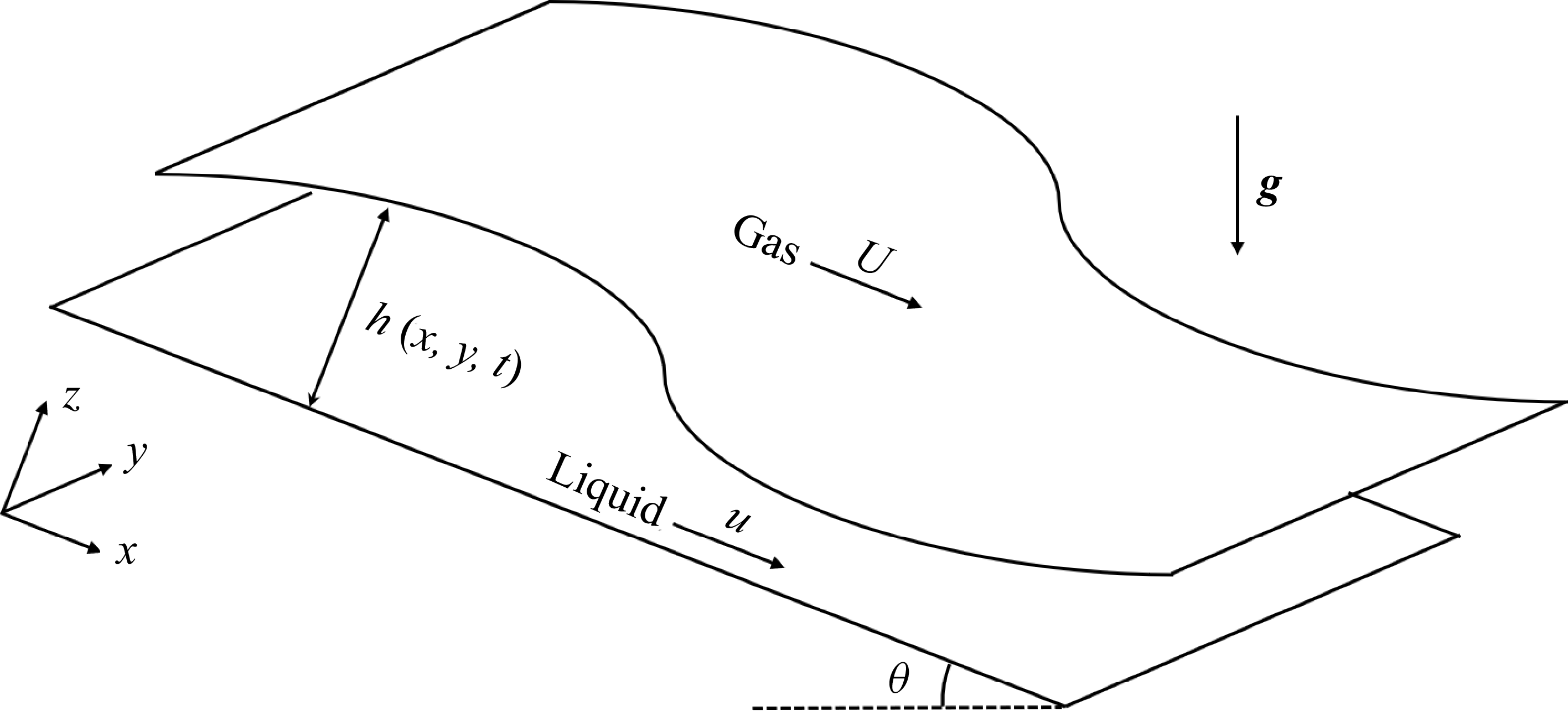
Sketch of the geometry of the gas–liquid flow problem, where
 $\boldsymbol{g}=(g\sin \theta ,0,-g \cos \theta )$
, with
 $g$
representing the acceleration due to gravity.

2. Mathematical formulation
The problem under investigation, as illustrated in figure 1, involves a liquid film with a free surface flowing down an inclined plane. The angle of inclination between the fixed wall and the horizontal plane is denoted by
 $\theta$
. A gas flow above the free surface interacts with the liquid film. We introduce the Cartesian coordinates
 $(x,y,z)$
, where the
 $x$
-direction corresponds to the flow direction, the
 $y$
-direction is aligned with the spanwise direction and the
 $z$
-direction is perpendicular to the undisturbed free surface. The fixed wall is located at
 $z=0$
, while the free surface of the liquid is described by
 $z=h(x,y,t)$
, where
 $t$
represents time.
This scenario involves a complex multiphase flow with a free interface, making it challenging to obtain a complete analytical solution. Simplifications are therefore necessary. A commonly adopted approach, initially proposed by Miles (Reference Miles1957) and Benjamin (Reference Benjamin1959), treats the gas flow as an independent problem. In their framework, the gas–liquid interface is approximated as a rigid boundary, and the gas flow is considered inviscid and quasi-laminar. This allows for the derivation of an expression that describes the pressure exerted by the gas on the gas–liquid interface. Following this, the fluid flow is assumed to be laminar, with the gas pressure at the interface serving as a boundary condition. This approach enables the development of various liquid flow models that are influenced by gas flow.
2.1. Gas problem
We denote the gas density by
 $\rho _a$
. For an undisturbed gas–liquid interface, the gas velocity is expressed as
 $\boldsymbol{U}= (U (z ),0,0 )$
. The wind velocity profile
 $U(z)$
is typically assumed to be either exponential or logarithmic, corresponding respectively to an asymptotic suction boundary-layer profile and a mean turbulent boundary-layer profile (Bonfils et al. Reference Bonfils, Mitra, Moon and Wettlaufer2022). When the liquid surface experiences a small perturbation, represented by
 $\eta$
, the gas flow velocity changes to
 $\boldsymbol{u}=\boldsymbol{U}+\overline {\boldsymbol{u}}$
, where
 $\overline {\boldsymbol{u}}= (u,v,w )$
represents the small perturbations added to the velocity field. The governing equations for the gas flow, which are the linearised Euler equations, are given by
 \begin{align} \boldsymbol{\nabla }\boldsymbol{\cdot }\overline {\boldsymbol{u}}=0\,,\quad \overline {\boldsymbol{u}}_t+U\overline {\boldsymbol{u}}_x+w\boldsymbol{U}_z=-\frac {\boldsymbol{\nabla }p}{\rho _a}, \end{align}
where
 $p$
is the pressure within the gas flow, and
 $\boldsymbol{\nabla }=(\partial _x,\partial _y,\partial _z)$
represents the spatial gradient operator. The kinematic boundary condition at the gas–liquid interface is satisfied as follows:
 \begin{align} w=\eta _t+U\eta _x\,,\quad \textrm{at}\;\;z=\overline {h}+\eta (x,y,t), \end{align}
where
 $\overline {h}$
is a constant representing the thickness of the liquid in the undisturbed state. Without loss of generality, we assume
 $k_x\gt 0$
and consider wave-like solutions
 \begin{align} \left \{u,v,w,p,\eta \right \}=\left \{\hat {u},\hat {v},\hat {w},\hat {p},\hat {\eta }\right \}e^{\mathrm{i}\big(k_xx +k_yy-k_xct\big)}+\textrm{c.c.} \end{align}
By substituting (2.3) into (2.1) and (2.2), we obtain
 \begin{align} \left . \begin{aligned} &\mathrm{i}k_x\hat {u}+\mathrm{i}k_y\hat {v}+\hat {w}_z=0\\[4pt]&\rho _a\left [\mathrm{i}k_x\left (U-c\right )\hat {u}+U_z\hat {w}\right ]=-\mathrm{i}k_x\hat {p}\\[4pt]&\rho _a\left [\mathrm{i}k_x\left (U-c\right )\hat {v}\right ]=-\mathrm{i}k_y\hat {p}\\[4pt]&\rho _a\left [\mathrm{i}k_x\left (U-c\right )\hat {w}\right ]=-\hat {p}_z \end{aligned} \right \}, \end{align}
and the kinematic boundary condition becomes
 \begin{align} \hat {w}=\mathrm{i}k_x\left (U-c\right )\hat {\eta }\,,\quad \textrm{at}\;\;z=\overline {h}. \end{align}
Here, the Squire transformation
 \begin{align} k^2=k_x^2+k_y^2\,,\quad k\widetilde {u}=k_x \widehat {u}+k_y\widehat {v}\,,\quad k\widetilde {x}=k_x x+k_y y\,,\quad \frac {\widetilde {p}}{k}=\frac {\widehat {p}}{k_x}\,,\quad \widetilde {w}=\widehat {w}\,,\quad \widetilde {c}=c , \end{align}
can be applied to reduce a 3-D fluid flow problem into an equivalent 2-D formulation
 \begin{align} \mathrm{i}k\widetilde {u}+\widetilde {w}_z=0\,,\quad \mathrm{i}k\left (U-c\right )\widetilde {u}+U_z\widetilde {w}=-\frac {\mathrm{i}k\widetilde {p}}{\rho _a}\,,\quad \mathrm{i}k\left (U-c\right )\widetilde {w}=-\frac {\widetilde {p}_z}{\rho _a}. \end{align}
Next, we introduce the streamfunction
 $\psi$
, which satisfies the relations
 $\widetilde {u}=-\psi _z$
and
 $\widetilde {w}=\mathrm{i}k\psi$
. By substituting the streamfunction into (2.7) and eliminating the pressure
 $p$
, we can obtain
 \begin{align} (U-c)\psi _{zz}-\big [k^2(U-c)+U_{zz}\big ]\psi =0. \end{align}
The variable substitution is then introduced
 \begin{align} \xi =\left \lvert k\right \rvert z\,,\quad \xi _0=\left \lvert k\right \rvert \overline {h}\,,\quad U-c=U_1V\left (\xi \right )\,,\quad \psi =U_1\frac {k_x}{k}\phi \left (\xi \right )\widehat {\eta }. \end{align}
Substituting (2.9) into (2.8) yields
 \begin{align} \frac {\text{d}^2\phi }{\text{d}\xi ^2}-\left (1+\frac {V_{\xi \xi }}{V}\right )\phi =0. \end{align}
Similarly, based on the streamfunction
 $\psi$
and change of variables (2.9), the boundary conditions can be recast to
 $\phi =V$
at
 $\xi =\xi _0$
and
 $\phi \to 0$
as
 $z\to \infty$
. The pressure exerted by the gas on the gas–liquid interface can be obtained from (2.7) as follows:
 \begin{align} \widetilde {p}_0=\rho _aU_1^2k_x\left (V\phi _{\xi }-V_{\xi }\phi \right )\hat {\eta }\,\Big |_{\xi =\xi _0}, \end{align}
where the value of
 $\phi$
is determined by (2.10), along with the boundary conditions. Without loss of generality, the term
 $V\phi _{\xi }-V_{\xi }\phi$
can be replaced with the complex quantity
 $\alpha +\mathrm{i}\beta$
. This allows extension of the previously derived 1-D pressure formulation at the boundary to the 2-D case. As a result, the expression for the force exerted by the gas on the liquid, when the 1-D interface is distorted into a 2-D surface, is given by
 \begin{align} \hat {p}_0=-\rho _aU_1^2\left (\alpha +\mathrm{i}\beta \right )\frac {k_x^2}{\sqrt {k_x^2+k_y^2}}\hat {\eta }, \end{align}
where
 $\alpha$
and
 $\beta$
are pressure coefficients. Both coefficients are real valued and depend on parameters such as the maximum wind speed and the underlying wind profile. The specific values of these coefficients were obtained by Conte & Miles (Reference Conte and Miles1959). According to their results, the magnitudes of these coefficients increase with the maximum wind speed, with
 $\alpha$
taking positive values and
 $\beta$
negative ones, and both parameters depending sensitively on the wind speed. It should also be noted that different wind velocity profiles affect only the values of the coefficients
 $\alpha$
and
 $\beta$
in (2.12), while the form of the pseudo-differential operator remains unchanged. In the present work, the primary interest lies not in the precise values of these coefficients, but in how the pseudo-differential operator in the pressure formulation influences the dynamics of film flows. Additionally, our wind-pressure model is a 2-D extension of the classical Miles theory (Miles Reference Miles1957). Upon reducing (2.12) to the 1-D limit, the resulting pressure expression recovers the operator forms employed by Miles (Reference Miles1957), Phillips (Reference Phillips1960) and King et al. (Reference King, Tuck and Vanden-Broeck1993), differing only in the specifics of coefficient evaluation. The final expression for pressure follows directly from (2.3) and (2.12)
 \begin{align}p_0=&\;-\rho _aU_1^2\left (\alpha +\mathrm{i}\beta \right )\frac {k_x^2}{\sqrt {k_x^2+k_y^2}}\hat {\eta }\exp \left [\mathrm{i}\big(k_xx+k_yy-k_xct\big)\right ]\nonumber\\ &\;-\rho _aU_1^2\left (\alpha -\mathrm{i}\beta \right )\frac {k_x^2}{\sqrt {k_x^2+k_y^2}}\hat {\eta }^*\exp \left [-\mathrm{i}\big(k_xx+k_yy-k_xct\big)\right ]. \end{align}
The derivation of (2.13) is fundamentally based on two conditions:
 $k_x\gt 0$
and the interface shape being represented by a single-mode triangular function. More generally, for
 $k_x\in \mathbb{R}$
and arbitrary interface shapes, the pressure exerted by the gas on the gas–liquid interface can be determined through the linear superposition nature of the Fourier transform
 \begin{align} p_w=-\rho _aU_1^2\int _{\mathbb{R}^2}\left [\alpha +\mathrm{i}\beta \,\,\mathrm{sgn}(k_x)\right ]\frac {k_x^2}{\sqrt {k_x^2+k_y^2}}\mathcal{F}\left [\eta \right ]\exp \left (\mathrm{i}k_xx+\mathrm{i}k_yy\right )\,\text{d}k_x\,\text{d}k_y, \end{align}
where
 $\,\mathrm{sgn}(\boldsymbol{\cdot })$
denotes the sign function and
 $\mathcal{F}[\boldsymbol{\cdot }]$
represents the Fourier transformation. We define the integral operator
 \begin{align} \mathcal{R}[f]=\frac {1}{2\pi }\mathrm{P.V.} \int _{\mathbb{R}^2}\frac {x^\prime }{\left (x^{\prime 2}+y^{\prime 2}\right )^{3/2}} f\left (x-x^\prime ,y-y^\prime \right ) \,\text{d}x^\prime \,\text{d}y^\prime , \end{align}
where the operator
 $\mathcal{R}$
represents the Riesz transformation, whose Fourier symbol is given by
 $\mathcal{F}[\mathcal{R}]=-\mathrm{i}k_x/\sqrt {k_x^2+k_y^2}$
(Stein Reference Stein2016). Accordingly, the pressure exerted by the air on the gas–liquid interface can be expressed as
 \begin{align} p_w=-\rho _aU_1^2\mathcal{R}\big [\alpha \eta _x +\beta \mathcal{H}(\eta _x)\big ], \end{align}
where
 $\mathcal{H}$
represents the Hilbert transform, defined as
 \begin{align} \mathcal{H}[f]=\frac {1}{\pi }\;\mathrm{P.V.}\int _{\mathbb{R}}\frac {f(x^{\prime },y)}{x^\prime -x}\,\text{d}x^\prime , \end{align}
with ‘P.V.’ denoting the Cauchy principal value.
2.2. Liquid problem
We consider the liquid to be a thin film of incompressible fluid. Therefore, the governing system for the liquid is the Navier–Stokes equations, expressed as
 \begin{align} \boldsymbol{\nabla }\boldsymbol{\cdot }\boldsymbol{u}=0\,,\qquad \frac {\partial \boldsymbol{u}}{\partial t}+\boldsymbol{u}\boldsymbol{\cdot }\boldsymbol{\nabla }\boldsymbol{u}=-\frac {1}{\rho }\boldsymbol{\nabla }p+\nu \varDelta \boldsymbol{u}+\boldsymbol{g}, \end{align}
where
 $\boldsymbol{u}= (u,v,w )$
represent the liquid velocity,
 $\rho$
is the liquid density,
 $\nu$
is the kinematic viscosity of the liquid and
 $\boldsymbol{g}= (g\sin \theta ,0,-g\cos \theta )$
is the gravitational acceleration vector. The liquid adheres to the no-slip and no-penetration boundary conditions at the bottom
 \begin{align} \boldsymbol{u}\left (x,y,z=0,t\right )=0. \end{align}
At the free surface of the liquid, the kinematic boundary condition should be satisfied with
 \begin{align} w=h_t+uh_x+vh_y, \quad \mbox{at}\quad z=h\left (x,y,t\right ), \end{align}
where
 $h=h (x,y,t )$
represents the thickness of the liquid. The balance of tangential and normal stresses at the gas–liquid interface requires that
 \begin{align} \big (1-h_x^2\big )\left (v_z+w_x\right )+2 (w_z-u_x)h_x-(u_y+v_x)h_y-(v_z+w_y)h_xh_y=0, \\[-28pt] \nonumber \end{align}
 \begin{align} \big (1-h_y^2\big )\left (v_z+w_y\right )+2 (w_z-v_y)h_y-(u_y+v_x)h_x-(u_z+w_x)h_xh_y=0, \\[0pt] \nonumber \end{align}
and
 \begin{align} \begin{aligned} &0=p_w-p-\frac {\sigma }{\big(1+h_x^2+h_y^2\big)^{3/2}}\big [\big (1+h_x^2\big )h_{yy}-2h_xh_yh_{xy}+\big (1+h_y^2\big )h_{xx}\big ]+\\&\frac {2\mu }{1+h_x^2+h_y^2}\big [u_xh_x^2+(u_y+v_x)h_xh_y+v_yh_y^2-(u_z+w_x)h_x-(v_z+w_y)h_y+w_z\big ], \end{aligned} \end{align}
where
 $\sigma$
is the surface tension coefficient,
 $\mu$
denotes the dynamic viscosity of the liquid and all variables are evaluated at
 $z=h$
. It is important to note that, since the viscosity of the gas is negligible, its effect on the liquid only contributes to the normal-stress balance in (2.23) and not to the tangential-stress balance in (2.21)–(2.22). When the liquid film flow is not influenced by wind, an exact solution exists with a uniform liquid thickness, corresponding to the well-known Nusselt flow (Kalliadasis et al. Reference Kalliadasis, Ruyer-Quil, Scheid and Velarde2012)
 \begin{align} \overline {h}=\overline {h}_N\,,\quad \overline {u}=\frac {g\sin \theta }{2\nu }\big (2\overline {h}_Nz-z^2\big )\,,\quad \overline {v}=\overline {w}=0\,,\quad \overline {p}=-\rho g\left (z-\overline {h}_N\right )\cos \theta , \end{align}
where the bars denote base states. The velocity at the free surface of the Nusselt flow, denoted as
 $\overline {u}_N=\overline {u}|_{z=\overline {h}_N}=g\overline {h}_N^2\sin \theta /2\nu$
, is chosen as the reference velocity. We introduce the following dimensionless quantities:
 \begin{align} Re=\frac {\overline {u}_N\overline {h}_N}{\nu }=\frac {g\overline {h}_N^3\sin \theta }{2\nu }\,,\quad W_d=\frac {\rho _aU_1^2}{\rho g \overline {h}_N\sin \theta }\,,\quad C=\frac {\overline {u}_N\mu }{\sigma }=\frac {\rho g \overline {h}_N\sin \theta }{2\sigma }, \end{align}
where
 $Re$
is the Reynolds number, measuring the ratio of inertial to viscous forces,
 $W_d$
is the wind-pressure parameter, measuring the ratio of the pressure exerted by the gas on the gas–liquid interface to the liquid pressure, and
 $C$
is the capillary number, measuring the ratio of surface tension to viscous pressure. We also implement the following dimensionless transformations:
 \begin{align} \left . \begin{aligned} &x^*=\frac {x}{\overline {h}_N},\quad y^*=\frac {y}{\overline {h}_N},\quad z^*=\frac {z}{\overline {h}_N},\quad \boldsymbol{u}^*=\frac {\boldsymbol{u}}{\overline {u}_N}\,,\\[5pt] &t^*=\frac {\overline {u}_N}{\overline {h}_N} t,\quad h^*=\frac {h}{\overline {h}_N},\quad \ p^*=\frac {\overline {h}_N}{\mu \overline {u}_N}\left (p+\rho g z \cos \theta \right )\,. \end{aligned} \right \} \end{align}
By substituting (2.26) into (2.18)–(2.23) and omitting the asterisks, we obtain
 \begin{align} \boldsymbol{\nabla }\boldsymbol{\cdot }\boldsymbol{u}=0\,,\qquad Re\left (\frac {\partial \boldsymbol{u}}{\partial t}+\boldsymbol{u}\boldsymbol{\cdot }\boldsymbol{\nabla }\boldsymbol{u}\right )=-\boldsymbol{\nabla }p+\Delta \boldsymbol{u}+2\boldsymbol{i}, \end{align}
where we have defined
 $\boldsymbol{i}= (1,0,0 )$
and
 $\varDelta =\boldsymbol{\nabla }\boldsymbol{\cdot }\boldsymbol{\nabla}$
representing the Laplace operator. The bottom boundary condition (2.19) and the gas–liquid interface boundary conditions (2.21)–(2.22) remain unchanged in form after non-dimensionalisation, while the normal-stress balance (2.23) transforms to
 \begin{align} 0 & = -W_d\mathcal{R}\left [\alpha h_x+\beta \mathcal{H}(h_x)\right ]-\tfrac {p}{2}+h\cot \theta -\frac {1}{2C\big (1+h_x^2+h_y^2\big )^{3/2}}\big [\big (1+h_x^2\big )h_{yy}\big . \nonumber\\[5pt]& \quad \big .-2h_xh_yh_{xy}+\big (1+h_y^2\big )h_{xx}\big ]+\frac {1}{1+h_x^2+h_y^2}\big [u_xh_x^2+(u_y+v_x)h_xh_y+v_yh_y^2\big .\nonumber\\[5pt]& \quad \big .-(u_z+w_x)h_x-(v_z+w_y)h_y+w_z\big ]. \end{align}
We introduce the long-wave assumption: the wavelength
 $\lambda$
of the surface waves on the liquid film is much greater than the thickness
 $\overline {h}_N$
of the undisturbed liquid film (Scheid, Ruyer-Quil & Manneville Reference Scheid, Ruyer-Quil and Manneville2006; Kalliadasis et al. Reference Kalliadasis, Ruyer-Quil, Scheid and Velarde2012). By setting
 $\epsilon =\overline {h}_N/\lambda \ll 1$
, we write
 \begin{align} x=\frac {x^*}{\epsilon }\,,\quad y=\frac {y^*}{\epsilon }\,,\quad t=\frac {t^*}{\epsilon }\,,\quad w=\epsilon w^*. \end{align}
By substituting (2.29) into (2.27) and removing the asterisks for ease of notation, we arrive at
 \begin{align} \boldsymbol{\nabla }\boldsymbol{\cdot }\boldsymbol{u}=0\,,\quad \epsilon Re\left [\frac {\partial \boldsymbol{u}}{\partial t}+(\boldsymbol{u}\boldsymbol{\cdot }\boldsymbol{\nabla })\boldsymbol{u}\right ]=-\epsilon \boldsymbol{\varLambda }\boldsymbol{\nabla }p+\epsilon ^2\left (\frac {\partial ^2\boldsymbol{u}}{\partial x^2}+\frac {\partial ^2\boldsymbol{u}}{\partial y^2}\right )+\frac {\partial ^2\boldsymbol{u}}{\partial z^2}+2\boldsymbol{i}, \end{align}
where
 $\boldsymbol{\varLambda }$
is a diagonal matrix with elements 1, 1 and
 $\epsilon ^{-2}$
along its main diagonal. In the same vein, the boundary conditions (2.21)–(2.22) and (2.28) are recast to
 \begin{align} \boldsymbol{u}\left (x,y,z=0,t\right )=0, \end{align}
and at
 $z=h (x,y,t )$
 \begin{align} w=h_t+uh_x+vh_y, \\[-28pt] \nonumber \end{align}
 \begin{align} \big (1-\epsilon ^2h_x^2\big )\big (u_z+\epsilon ^2 w_x\big )+2\epsilon ^2\left (w_z-u_x\right )h_x-\epsilon ^2(u_y+v_x)h_y-\epsilon ^2 \big (v_z+\epsilon ^2 w_y\big )h_xh_y=0, \\[-28pt] \nonumber \end{align}
 \begin{align} \big (1-\epsilon ^2h_y^2\big )\big (v_z+\epsilon ^2 w_y\big )+2\epsilon ^2(w_z-v_y)h_y-\epsilon ^2(u_y+v_x)h_x-\epsilon ^2\big (u_z+\epsilon ^2w_x\big )h_xh_y=0, \\[0pt] \nonumber \end{align}
and
 \begin{align} 0 & = -\epsilon W_d\mathcal{R}\big [ \alpha h_x +\beta \mathcal{H}(h_x)\big ]-\tfrac {p}{2}+h\cot \theta -\frac {\epsilon ^2}{2C\big (1+\epsilon ^2h_x^2+\epsilon ^2h_y^2\big )^{3/2}}\big [\big (1+\epsilon ^2h_x^2\big )h_{yy}\big . \nonumber\\& \quad \big .-2\epsilon ^2h_xh_yh_{xy}+\big (1+\epsilon ^2h_y^2\big )h_{xx}\big ]+\frac {\epsilon }{1+\epsilon ^2h_x^2+\epsilon ^2h_y^2}\big [\epsilon ^2u_xh_x^2 +\epsilon ^2(u_y+v_x)h_xh_y\big .\nonumber\\& \quad \big .+\epsilon ^2v_yh_y^2-\big (u_z+\epsilon ^2w_x\big )h_x-\big (v_z+\epsilon ^2w_y\big )h_y+w_z\big ]. \end{align}
Next, we present the following asymptotic expansions for the thickness, velocity, and pressure of the liquid:
 \begin{align} \{h,u,v,w,p\} & = \{h_0,u_0,v_0,w_0,p_0\}+\epsilon \{h_1,u_1,v_1,w_1,p_1\} \nonumber \\ & \quad +\epsilon ^2\{h_2,u_2,v_2,w_2,p_2\}+{\cdots} . \end{align}
Assuming the dimensionless parameters
 $C\sim O (\epsilon ^2 )$
and
 $W_d\sim O (1/\epsilon )$
, we introduce new dimensionless parameters defined as follows:
 \begin{align} \overline {C}=\frac {C}{\epsilon ^2}\,,\qquad \overline {W}_d=\epsilon W_d, \end{align}
where
 $\overline {C}$
and
 $\overline {W}_d$
are
 $O (1 )$
quantities. We also assume that the Reynolds number
 $Re$
is of
 $O (1 )$
. After applying the asymptotic expansions, the leading-order terms from (2.30) to (2.35) yield
 \begin{align} u_{0x}+v_{0y}+w_{0z}=0\,,\quad u_{0zz}=-2\,,\quad v_{0zz}=0,\quad p_{0z}=0, \end{align}
subject to the boundary conditions
 \begin{align} u_0=v_0=w_0=0\,,\quad \text{at}\;\;y=0, \end{align}
and at
 $y=h_0$
, with
 \begin{align} u_{0z}=0\,,\quad v_{0z}=0\,,\quad p_0=2\left [h_0\cot \theta -\overline {W}_d\mathcal{R}\left [ \alpha h_{0x} +\beta \mathcal{H}(h_{0x})\right ]-\frac {1}{2\overline {C}}\varDelta h_0\right ]. \end{align}
The solution to the leading-order problem represented by (2.38)–(2.40) is given by
 \begin{align} \left . \begin{aligned} &u_0=\left (2h_0-z\right )z\,,\quad v_0=0\,,\quad w_0=-z^2h_{0x}\,,\\[5pt]&p_0=2\left [h_0\cot \theta -\overline {W}_d\mathcal{R}\big [ \alpha h_{0x} +\beta \mathcal{H}(h_{0x})\big ]-\frac {1}{2\overline {C}}\varDelta h_0\right ]\,. \end{aligned} \right \} \end{align}
Equations (2.41) demonstrate that the leading-order pressure is independent of
 $z$
. This observation is consistent with Prandtl’s boundary-layer theory, which states that pressure remains constant throughout the boundary layer. For the leading-order terms, the kinematic boundary condition can be expressed as
 \begin{align} h_{0t}+2h_0^2\,h_{0x}=0. \end{align}
At the next-to-leading order, a similar approach is employed to solve the problem. Here, we present the solution directly, without detailing the mathematical derivation
 \begin{align} \left . \begin{aligned} &u_1=\left (\frac 12z^2-zh_0\right )p_{0x}+Re\left (\frac {1}{6}z^4h_0-\frac 23z^3h_0^2+\frac 43zh_0^4\right )h_{0x}+2zh_1\,,\\[5pt]&v_1=\left (\frac {1}{2}z^2-zh_0\right )p_{0y}\,,\quad w_1=-\int _{0}^{z}\left (u_{1x}+v_{1y}\right )\text{d}z\,. \end{aligned} \right \} \end{align}
The kinematic boundary condition leads to a Burgers-type equation
 \begin{align} h_{1t}+\left (2h_0^2h_1+\frac {8}{15}Reh_0^6h_{0x}-\frac 13h_0^3p_{0x}\right )_x+\left (-\frac 13h_0^3p_{0y}\right )_y=0. \end{align}
By defining
 $H=h_0+\epsilon h_1$
and combining (2.42) with
 $\epsilon$
times (2.44), we obtain
 \begin{align} \begin{aligned} H_t+\boldsymbol{\nabla} _\perp \boldsymbol{\cdot }&\;\left \{\left (\frac 23H^3+\frac {8}{15}\epsilon ReH^6H_x\right )\boldsymbol{i}_\perp \right .\\[5pt]&\;\left .-\frac 23\epsilon H^3\boldsymbol{\nabla} _\perp \left [H\cot \theta -\overline {W}_d\mathcal{R}\big [ \alpha H_x+\beta \mathcal{H}(H_x)\big ]-\frac {1}{2\overline {C}\varDelta _\perp H}\right ]\right \}=0\,, \end{aligned} \end{align}
where
 $\boldsymbol{\nabla} _\perp =(\partial _x,\partial _y)$
and
 $\varDelta _\perp =\partial _{xx}+\partial _{yy}$
are the 2-D gradient and Laplace operators, respectively, and
 $\boldsymbol{i}_\perp =(1,0)$
. It is noted that, when
 $\overline {W}_d=0$
, this equation reduces to the well-known Benney equation (Benney Reference Benney1966a
; Kalliadasis et al. Reference Kalliadasis, Ruyer-Quil, Scheid and Velarde2012). The solution to the Benney equation may exhibit finite-time blow-up (Pumir, Manneville & Pomeau Reference Pumir, Manneville and Pomeau1983; Rosenau, Oron & Hyman Reference Rosenau, Oron and Hyman1992; Scheid et al. Reference Scheid, Ruyer-Quil, Thiele, Kabov, Legros and Colinet2005; Kalliadasis et al. Reference Kalliadasis, Ruyer-Quil, Scheid and Velarde2012); thus, we further investigate the weakly nonlinear evolution of small perturbations to the uniform state. We substitute
 $H=1+\epsilon \eta$
into (2.45), treating
 $\eta \sim O(1)$
. Assuming that
 $\cot \theta \sim O(1)$
, we then apply the variable substitutions
 \begin{align} \bar {t}=4\epsilon t\quad \text{and}\quad \bar {x}=x-2t, \end{align}
subsequently dropping bars for simplicity. This leads us to the Nepomnyashchy-type equation
 \begin{align} \eta _t+\eta \eta _x+\frac {2Re}{15}\eta _{xx}-\frac {\cot \theta }{6}\varDelta _\perp \eta +\frac {\overline {W}_d}{6}\varDelta _\perp \mathcal{R}\big [\alpha \eta _x +\beta \mathcal{H}(\eta _x)\big ]+\frac {1}{12\overline {C}}\varDelta _\perp ^2\eta =0. \end{align}
In this paper, we restrict our study to the case where
 $\cot \theta \gt 0$
and
 $\cot \theta \sim O(1)$
. We rescale (2.47) using the transformations
 \begin{align} \left . \begin{aligned} &t^*=\frac {\cot ^2\theta \overline {C}}{3}t\,,\quad x^*=\sqrt {2\overline {C}\cot \theta }x\,,\quad y^*=\sqrt {2\overline {C}\cot \theta }y,\quad r^*=\frac {4Re}{5\cot \theta }\,,\\ &\eta ^*=\frac {3\sqrt {2}}{\sqrt {\overline {C}\cot ^3\theta }}\eta \,,\quad \alpha ^*=\sqrt {\frac {2\overline {C}}{\cot \theta }}\overline {W}_d\,,\quad \beta ^*=\sqrt {\frac {2\overline {C}}{\cot \theta }}\overline {W}_d\beta \,, \end{aligned} \right \} \end{align}
and then drop the asterisks. This results in the following canonical equation:
 \begin{align} \eta _t+\eta \eta _x+(r-1)\eta _{xx}-\eta _{yy}+\varDelta _\perp \mathcal{R}\big [ \alpha \eta _x +\beta \mathcal{H}(\eta _x)\big ]+\varDelta _\perp ^2\eta =0, \end{align}
where
 $r\gt 0$
is the equivalent Reynolds number, and
 $\alpha \geqslant 0$
and
 $\beta \leqslant 0$
are wind-pressure parameters. It is noted that when both
 $\alpha$
and
 $\beta$
are equal to zero, the equation reduces to the Nepomnyashchy equation (Kalliadasis et al. Reference Kalliadasis, Ruyer-Quil, Scheid and Velarde2012).
3. Primary instability
By linearising (2.49), we obtain
 \begin{align} \eta _t+(r-1)\eta _{xx}-\eta _{yy}+\varDelta _\perp \mathcal{R}\big [\alpha \eta _x+\beta \mathcal{H}(\eta _x)\big ]+\varDelta _\perp ^2\eta =0. \end{align}
For the wavenumber vector
 $(k_x,k_y)$
and the complex frequency
 $\lambda$
, substituting the ansatz
 $e^{\mathrm{i}k_xx+\mathrm{i}k_yy+\lambda t}$
into (3.1) yields the linear dispersion relation given by
 \begin{align} \lambda =(r-1)k_x^2-k_y^2+\left [\alpha +\mathrm{i}\beta \,\mathrm{sgn}(k_x)\right ]k_x^2\sqrt {k_x^2+k_y^2}-\big(k_x^2+k_y^2\big)^2. \end{align}
We can decompose this dispersion relation into its real and imaginary components as
 \begin{align} \lambda ^r=(r-1)k_x^2-k_y^2+\alpha k_x^2\sqrt {k_x^2+k_y^2}-\big(k_x^2+k_y^2\big)^2 , \end{align}
and
 \begin{align} \lambda ^i=\beta \,\mathrm{sgn}(k_x) k_x^2\sqrt {k_x^2+k_y^2}, \end{align}
where
 $\lambda ^r$
and
 $\lambda ^i$
denote the real and imaginary parts of
 $\lambda$
, respectively, with
 $\alpha \geqslant 0$
and
 $\beta \leqslant 0$
. In this context,
 $\lambda ^r$
indicates the growth rate of small-amplitude waves, while
 $\lambda ^i$
relates to the phase speed
 $\boldsymbol{c}_p$
, represented by
 \begin{align} \boldsymbol{c}_p=\left (-\beta \left \lvert k_x\right \rvert \sqrt {k_x^2+k_y^2}\,,\;\;-\beta \frac {k_x^2}{k_y}\,\mathrm{sgn}(k_x)\sqrt {k_x^2+k_y^2}\right ). \end{align}
The condition
 $\beta \leqslant 0$
suggests that wind has a positive contribution to the phase speed. As
 $\left \lvert \beta \right \rvert$
increases, the magnitude of the phase speed also rises. However, it is important to note that this analysis involves a Galilean transformation (as referenced in (2.46)). This implies that when transitioning to a reference frame relative to the Earth, the wind’s impact on the phase speed is only an
 $\mathcal{O}(\epsilon )$
quantity. According to Miles’ theory, given a specific wind velocity profile, the values of
 $\alpha$
and
 $\beta$
are solely determined by the phase speed of water waves (Miles Reference Miles1957; Kharif et al. Reference Kharif, Kraenkel, Manna and Thomas2010). Since the correction to the phase speed due to wind is only an
 $\mathcal{O}(\epsilon )$
quantity, we can reasonably treat
 $\alpha$
and
 $\beta$
as predetermined constants in subsequent analyses.
Next, we consider
 $\lambda ^r$
, which denotes the growth rate of small-amplitude linear waves. The instability of the flow is driven by the wind-pressure parameter
 $\alpha$
, representing the component of the normal pressure in phase with the wave elevation. This mechanism corresponds to class C in the classification by Benjamin (Reference Benjamin1963), specifically the Kelvin–Helmholtz type. When
 $\lambda ^r\gt 0$
, it suggests that the wave is unstable, indicating primary instability where the wave amplitude will increase over time. Conversely, if
 $\lambda ^r\lt 0$
, the wave amplitude is expected to decay over time. It is essential to note that this discussion is an approximation within the linear regime. Therefore, even if
 $\lambda ^r\gt 0$
, it does not imply that the wave amplitude will increase indefinitely. As the wave amplitude grows, nonlinear effects can become significant, potentially limiting further growth and leading to a stable state, a process known as nonlinear saturation. Moreover, waves that achieve nonlinear saturation may still become unstable under specific perturbations, such as transverse disturbances, leading to what is known as secondary instability. Assuming
 $k=\sqrt {k_x^2+k_y^2}$
, we have
 $(k_x,k_y)=(k\cos \theta ,k\sin \theta )$
. Substituting this variable transformation into (3.3) yields
 \begin{align} \lambda ^r\big(k,\theta \big)=rk^2\cos ^2\theta +\alpha k^3\cos ^2\theta -k^2-k^4, \end{align}
where
 $r\gt 0$
and
 $\alpha \geqslant 0$
. Therefore, when
 $\lambda ^r (k,\theta )$
reaches its maximum value,
 $\theta$
must be 0. This indicates that the most unstable mode in primary instability is always the 1-D streamwise mode. Consequently, we will consider only the 1-D case, reducing
 $\lambda ^r$
to
 \begin{align} \lambda ^r(k)=(r-1)k^2+\alpha k^3-k^4. \end{align}
Effects of wind on the growth rate. (
 $a$
) Supercritical flow with
 $r=2$
and various values of
 $\alpha$
:
 $\alpha =0$
(blue solid line),
 $\alpha =1$
(red dash-dotted line) and
 $\alpha =2$
(green dashed line). (
 $b$
) Subcritical flow with
 $r=0.01$
and various values of
 $\alpha$
:
 $\alpha =0$
(blue solid line),
 $\alpha =2.03$
(red dash-dotted line) and
 $\alpha =2.1$
(green dashed line).

It is evident that wind consistently contributes to wave instability, as demonstrated in (3.7). In the absence of wind (i.e.
 $\alpha =0$
), for
 $0\lt r\leqslant 1$
, it follows that
 $\lambda ^r\leqslant 0$
for all values of
 $k$
, indicating all modes are stable. However, for
 $r\gt 1$
,
 $\lambda ^r(k)\gt 0$
signifies that instability arises for
 $0\lt k\lt \sqrt {r-1}$
. Notably,
 $r=1$
corresponds to the critical Reynolds number, denoted as
 $Re_c=5\cot \theta /4$
(Benney Reference Benney1966b
). In this paper, flows with
 $r\gt 1$
are classified as supercritical, those with
 $r\lt 1$
as subcritical, and those with
 $r=1$
as critical.
When wind is present, for supercritical and critical flows (i.e.
 $r\geqslant 1$
), the condition
 $\alpha ^2+4(r-1)\geqslant 0$
is always satisfied. This indicates that there are unstable modes for
 \begin{align} 0\lt k\lt \frac {\alpha +\sqrt {\alpha ^2+4(r-1)}}{2}, \end{align}
with the most unstable mode occurring at
 \begin{align} k_u=\frac {3\alpha +\sqrt {9\alpha ^2+32(r-1)}}{8}. \end{align}
As the parameter
 $\alpha$
increases, the bandwidth of unstable modes, the wavenumber of the most unstable mode, and the maximum growth rate also increase. Representative results are illustrated in figure 2(
 $a$
). For flows with subcritical Reynolds numbers (i.e.
 $0\lt r\lt 1$
), if
 $0\lt \alpha \lt 2\sqrt {1-r}$
, then
 $\lambda ^r (k)\leqslant 0$
for all
 $k$
, indicating that all modes are stable. However, if
 $\alpha \gt 2\sqrt {1-r}$
, unstable modes appear within the range
 \begin{align} \frac {\alpha -\sqrt {\alpha ^2+4(r-1)}}{2}\lt k\lt \frac {\alpha +\sqrt {\alpha ^2+4(r-1)}}{2}, \end{align}
with the most unstable mode again occurring at
 $k_u$
given by (3.9). As
 $\alpha$
increases, the bandwidth of these unstable modes, the wavenumber of the most unstable mode, and the maximum growth rate continue to rise, as shown in figure 2(
 $b$
). From this analysis, we can draw the following conclusions.
-
(i) Wind enhances the primary instability.
-
(ii) When
 $0\lt r\lt 1$
, there exists a critical value for
$\alpha$
, denoted as
$\alpha _c=2\sqrt {1-r}$
. If
$\alpha \lt \alpha _c$
, all modes are stable; if
$\alpha \gt \alpha _c$
, unstable modes are present.
-
(iii) There exists an upper critical wavenumber
(3.11)which defines a necessary condition for primary instability. Unstable modes can only arise for wavenumbers satisfying
\begin{align} k^+=\frac {\alpha +\sqrt {\alpha ^2+4(r-1)}}{2}, \end{align}
$k\lt k^+$
.


4. Nonlinear travelling waves
The linear stability analysis previously presented indicates that the most unstable mode during primary instability is always the 1-D streamwise (longitudinal) mode. Therefore, this section focuses on the examination of a 1-D travelling wave, as described by (2.49). The investigation is conducted in a reference frame that moves with the velocity
 $c$
of the travelling wave; thus, the wave becomes steady in this new frame. To obtain a 1-D steady solution, we derive the following expression from (2.49):
 \begin{align} -c\eta _x+\eta \eta _x+(r-1)\eta _{xx}-\alpha \mathcal{H}\left [\eta _{xxx}\right ]+\beta \eta _{xxx}+\eta _{xxxx}=0. \end{align}
Here, we concentrate on two distinct types of travelling waves:
 $\gamma _1$
waves and
 $\gamma _2$
waves. The
 $\gamma _1$
wave propagates at a speed slower than that of an infinitesimal periodic wave, while the
 $\gamma _2$
wave propagates at a faster speed (Chang & Demekhin Reference Chang and Demekhin2002; Kalliadasis et al. Reference Kalliadasis, Ruyer-Quil, Scheid and Velarde2012). For a periodic wave, we assume that the mass flow is constant, expressed mathematically as
 \begin{align} \frac {1}{2L}\int _{-L}^{L}\eta \,\text{d}x=0, \end{align}
where
 $L$
denotes half the length of the computational domain. By integrating (4.1) once, we can derive that
 \begin{align} -c\eta +\frac 12\eta ^2+(r-1)\eta _{x}-\alpha \mathcal{H}\left [\eta _{xx}\right ]+\beta \eta _{xx}+\eta _{xxx}=C_1, \end{align}
where
 $C_1$
is an unknown integral constant. Additionally, we impose a pinning condition,
 $\eta _x|_{x=x_0}=0$
, to eliminate the translational invariance of the solution. This system of equations is solved numerically in a periodic domain
 $[-L,L]$
using a pseudo-spectral method coupled with a Newton–Raphson iteration scheme. Convergence is prescribed by a residual tolerance of
 $10^{-10}$
in the
 $l^\infty$
-norm. To ensure resolution independence, the numerical scheme was tested across a hierarchy of discretisations (512, 1024 and 2048 nodes per wavelength). For the majority of the travelling-wave computations, a resolution of 1024 was adopted, as further refinement yielded no discernible change in the solution profiles within the prescribed numerical precision. For convenience, we introduce a normalised wavenumber
 $k^*=k/k^+$
, where
 $k^+$
is the upper critical wavenumber.
Figure 3 displays the bifurcation diagram of wave speed
 $c$
versus normalised wavenumber
 $k^*$
, along with representative wave profiles. At
 $k^*=1$
, the solution corresponds to an infinitesimal periodic wave, with its wave speed precisely determined by (3.5). The bifurcation diagram reveals two distinct branches of periodic waves: the
 $\gamma _1$
branch, characterised by wave speeds lower than that of the infinitesimal wave, and the
 $\gamma _2$
branch, which has higher wave speeds. The
 $\gamma _1$
branch bifurcates from the Nusselt flat-film solution at
 $k^*=1$
, suggesting a Hopf bifurcation, while the
 $\gamma _2$
branch emerges near
 $k^*=1/2$
, indicative of a period-doubling bifurcation (Chang & Demekhin Reference Chang and Demekhin2002).
In terms of wave profiles,
 $\gamma _1$
waves exhibit a prominent depression, while
 $\gamma _2$
waves display a notable elevation. Wind pressure has a significant impact on the
 $k^*-c$
bifurcation diagrams. As
 $\alpha$
increases, the
 $\gamma _1$
branch rotates counterclockwise about a point near
 $c=0$
. This implies that, for large
 $k^*$
values, a higher
 $\alpha$
leads to a faster
 $\gamma _1$
wave, whereas, for small
 $k^*$
values, a higher
 $\alpha$
reduces the wave speed. For
 $\gamma _2$
waves at a fixed
 $k^*$
, increasing
 $\alpha$
consistently increases the wave speed. The dispersive parameter
 $\beta$
also plays a crucial role in shaping the
 $k^*-c$
curves. When
 $\beta =0$
, the bifurcation curves for
 $\gamma _1$
and
 $\gamma _2$
waves are approximately symmetric around
 $c=0$
. However, this symmetry is broken when dispersion is introduced. For large
 $k^*$
, stronger dispersion (i.e. more negative
 $\beta$
) leads to an increase in wave speed; conversely, for small
 $k^*$
, stronger dispersion results in a decrease in wave speed. In later sections, we will explore other bifurcation diagrams, such as those in
 $r{-}c$
and
 $\beta\!-\!c$
spaces, which will reveal additional wave branches. Nevertheless, our subsequent analyses of secondary instability will focus on periodic waves located along the
 $k^*-c$
bifurcation curves.
Effects of wind parameters on the
 $k^*-c$
bifurcation curves for
 $\gamma _1$
and
 $\gamma _2$
waves.
 $(a)$
The influence of the parameter
 $\alpha$
at a fixed value of
 $r=2$
and
 $\beta =-0.2$
. The curves correspond to
 $\alpha =0.8$
(blue dashed line),
 $\alpha =2$
(red solid line) and
 $\alpha =2$
(green dash-dotted line).
 $(b)$
The influence of the parameter
 $\beta$
at a fixed value of
 $r=2$
and
 $\alpha =1$
. The curves represent
 $\beta =0$
(blue dashed line),
 $\beta =-0.1$
(red solid line) and
 $\beta =-0.2$
(green dash-dotted line).
 $(c)$
Wave profiles of
 $\gamma _1$
corresponding to the circles in panel
 $(a)$
.
 $(d)$
Wave profiles of
 $\gamma _2$
corresponding to the circles in panel
 $(a)$
.

Effects of wind parameters on the
 $r{-}c$
diagrams for
 $\gamma _2$
waves.
 $(a)$
With
 $\beta$
fixed at 0 and
 $\alpha$
varying:
 $\alpha =0$
(blue),
 $\alpha =1$
(red) and
 $\alpha =2$
(green).
 $(b)$
With
 $\alpha$
fixed at 1 and
 $\beta$
varying:
 $\beta =0$
(green),
 $\beta =-0.2$
(blue) and
 $\beta =-0.4$
(red).
 $(c)$
Wave profiles corresponding to the circles in panel
 $(b)$
.

Figures 4
 $(a)$
and 4
 $(b)$
display the bifurcation curves of the equivalent Reynolds number
 $r$
and wave speed
 $c$
for periodic
 $\gamma _2$
waves under different wind-pressure parameters
 $\alpha$
and
 $\beta$
, along with the typical wave profiles for
 $L=100$
. It is evident that the
 $r{-}c$
curves for varying wind-pressure parameters follow a similar trend: a larger equivalent Reynolds number is associated with a higher wave speed and increased wave height. The turning point of the
 $r{-}c$
curve occurs slightly to the right of the critical equivalent Reynolds number,
 $r_c=1-\alpha ^2/4$
. This is reasonable because for
 $r\lt r_c$
, the condition
 $\alpha ^2+4(r-1)\lt 0$
holds, indicating that all perturbations will decay to zero, based on previous instability analysis.
Furthermore, the wind-pressure parameter
 $\alpha$
causes a leftward shift of the
 $r{-}c$
curve. For a given equivalent Reynolds number, a larger
 $\alpha$
corresponds to a higher wave speed. An increase in
 $\alpha$
also leads to the emergence of self-intersecting structures in the
 $r{-}c$
curve. Along this curve, the wave profiles are locally confined, featuring oscillatory decaying tails (see figure 4(c)). In our study, we computed bifurcation curves for the wind-pressure parameter
 $\alpha$
and the wave speed
 $c$
, and found that they closely resemble those in the
 $r{-}c$
diagrams; therefore, these results are omitted here. In contrast, the wind-pressure parameter
 $\beta$
induces a rightward shift of the bifurcation curve, but this only applies to small variations of
 $\beta$
. In addition, the parameter
 $\beta$
suppresses the formation of the self-intersecting structure in the
 $r{-}c$
curve.
 $(a)$
The
 $\beta\!-\!c$
bifurcation curve for
 $\gamma _2$
waves at
 $r=3$
and
 $\alpha =1$
.
 $(b)$
Representative wave profiles corresponding to the circles in panel
 $(a)$
.

The influence of the wind-pressure parameter
 $\beta$
exhibits considerable complexity. For
 $r=3$
and
 $\alpha =1$
, the
 $\beta\!-\!c$
bifurcation curve for periodic
 $\gamma _2$
waves is presented in figure 5
 $(a)$
. This curve displays a distinct ‘snake-like’ structure, with multiple inflexion points and an overall shape resembling ‘wings’. It is noteworthy that, as indicated by Conte & Miles (Reference Conte and Miles1959), the parameter
 $\beta$
must remain negative. Consequently, the segment of the
 $\beta\!-\!c$
bifurcation curve where
 $\beta \gt 0$
is of purely mathematical interest and does not present physically realisable situations. Figure 5
 $(b)$
illustrates the typical wave profiles. As
 $c\rightarrow 0$
along the
 $\beta\!-\!c$
curve, the wave profiles at the turning points of the curve show broader oscillations.
We also identified
 $\gamma _1$
waves, which are characterised by a wave speed that is lower than that of an infinitesimal periodic wave. Figures 6
 $(a)$
and 6
 $(b)$
illustrate the
 $r{-}c$
bifurcation curves for periodic
 $\gamma _1$
waves for
 $L=100$
under varying wind-pressure parameters
 $\alpha$
and
 $\beta$
, while figure 6
 $(c)$
presents typical wave profiles. The effects of the wind-pressure parameters on the
 $r{-}c$
diagram for
 $\gamma _1$
waves exhibit similarities to their influence on the
 $r{-}c$
diagram for
 $\gamma _2$
waves. The turning points of the
 $r{-}c$
curve for
 $\gamma _1$
waves are located near the right side of the critical equivalent Reynolds number
 $r_c=1-\alpha ^2/4$
. The wind-pressure parameter
 $\alpha$
causes a leftward shift in the
 $r{-}c$
curve for
 $\gamma _1$
waves, and an increase in
 $\alpha$
leads to the emergence of self-intersecting structures within this curve. In contrast, the wind-pressure parameter
 $\beta$
results in a rightward shift of the
 $r{-}c$
curve for
 $\gamma _1$
waves, although this effect is observed only for small variations in
 $\beta$
. Furthermore, the parameter
 $\beta$
suppresses the formation of self-intersecting structures in the
 $r{-}c$
curve for
 $\gamma _1$
waves.
Effects of wind parameters on the
 $r{-}c$
bifurcation curves for
 $\gamma _1$
waves.
 $(a)$
With
 $\beta$
fixed at 0 and
 $\alpha$
varying:
 $\alpha =0$
(blue),
 $\alpha =1$
(red) and
 $\alpha =2$
(green).
 $(b)$
With
 $\alpha$
fixed at 1 and
 $\beta$
varying:
 $\beta =0$
(green),
 $\beta =-0.2$
(blue) and
 $\beta =-0.4$
(red).
 $(c)$
Wave profiles corresponding to the circles in panel
 $(b)$
.

 $(a)$
The
 $\beta\!-\!c$
bifurcation curve for
 $\gamma _1$
waves at
 $r=3$
and
 $\alpha =1$
.
 $(b)$
Representative wave profiles corresponding to the circles in panel
 $(a)$
.

The
 $\beta\!-\!c$
bifurcation curve for periodic
 $\gamma _1$
waves, illustrated in figure 7
 $(a)$
for
 $r=3$
and
 $\alpha =1$
, shares qualitative similarities to that of periodic
 $\gamma _2$
waves. Both bifurcation curves display a ‘snake-like’ structure with multiple turning points. In the present study, attention is restricted to the segment of the bifurcation curve where
 $\beta \lt 0$
, in accordance with the findings of Conte & Miles (Reference Conte and Miles1959). Figure 7
 $(b)$
presents a selection of typical wave profiles associated with
 $\gamma _1$
waves. As
 $c\rightarrow 0$
along the
 $\beta\!-\!c$
curve, the wave profiles at the turning points exhibit broader oscillations.
5. Secondary instability
In the previous section, we provided numerical computations of 1-D travelling-wave solutions of (2.49). In this section, we will examine their secondary instabilities.
5.1. Secondary instability of
$\gamma _1$
waves

Numerical computations indicate that
 $\gamma _1$
waves bifurcate near the upper critical wavenumber, given by
 $k^+=1/2 [\alpha +\sqrt {\alpha ^2+4(r-1)} ]$
. This section focuses on analysing the stability of those
 $\gamma _1$
waves close to
 $k^+$
. To facilitate this analysis, we first derive asymptotic solutions of (4.1) in the form
 \begin{align} \eta _s=A_k\exp (\mathrm{i}kx)+A_{2k}\exp (2\mathrm{i}kx)+\textrm{c.c.}, \end{align}
where
 $c=-\beta k^2$
and
 \begin{align} \left .\begin{aligned} &\left |A_k\right |^2=-4k^2\big [(r-1)+\alpha \left |k\right |-k^2\big ]\big [ (r-1)+2\alpha \left |k\right |-4k^2\big ]\\&A_{2k}=\mathrm{i}k\big (r-1+\alpha \left |k\right |-k^2\big ) \end{aligned} \right \}, \end{align}
with
 $A_k$
and
 $A_{2k}$
being purely imaginary, giving that
 $\eta (0)=0$
. Upon noting that the amplitude of the periodic
 $\gamma _1$
waves near the upper critical wavenumber
 $k^+$
satisfies
 $A_k\ll 1$
and
 $A_{2k}\sim O(A_k^2)$
, we introduce the Fourier expansion of
 $\eta$
in terms of
 $x$
 \begin{align} \eta =\int A_k\left (t\right )\exp (\mathrm{i}kx)\,\text{d}k+\textrm{c.c.}, \end{align}
where
 $A_k$
is the complex amplitude and
 $A_0$
is identically zero due to mass conservation. Substituting (5.3) into (2.49), the nonlinear terms immediately give rise to resonance conditions associated with a specific mode
 $A_k(t)$
 \begin{align} k\pm l\pm m=0\,,\qquad k\pm l\pm m\pm n=0, \end{align}
corresponding to cubic and quartic interactions, respectively. The choice of specific wave-mode combinations depends on the problem being addressed, and this selection determines the corresponding amplitude evolution equations. Considering the evolution of a single Fourier mode
 $A_k$
leads to the well-known Stuart–Landau equation
 \begin{align} \frac{\text{d}A_k}{\text{d}t}=\lambda _k A_k +\frac {k^2}{\lambda _{2k}-\lambda _{k}}\left |A_k\right |^2 A_k, \end{align}
where
 $\lambda _k=(r-1)k^2+\alpha \lvert k\rvert ^3-k^4+\mathrm{i}\beta k^3$
, describing the interaction between the fundamental mode
 $k$
, its first overtone mode
 $2k$
, and itself. This equation admits a saturated solution
 $\eta _s$
as given in (5.1). When
 $\eta _s$
is subjected to streamwise disturbances at overtones of
 $k$
, linearising (5.5) around
 $\eta _s$
yields the secondary growth rate
 \begin{align} g_1=-2\lambda _k^r=-2\big [(r-1)k^2+\alpha \left \lvert k\right \rvert ^3-k^4\big ]\lt 0. \end{align}
Therefore,
 $\eta _s$
for the
 $\gamma _1$
waves near the upper critical wavenumber
 $k^+$
remains stable under streamwise (i.e. longitudinal) overtone disturbances. This indicates that the secondary instability of
 $\eta _s$
induced by longitudinal disturbances does not arise from its overtone perturbations, but rather from non-overtone disturbances. Since (5.5) does not account for instabilities stemming from non-overtone perturbations of the fundamental mode, it is necessary to establish a mechanism for the instability of
 $\eta _s$
induced by non-harmonic modes. To address this, consider a non-harmonic mode
 $A_m$
, where
 $m$
is not an integer multiple of
 $k$
. We introduce a multi-mode asymptotic expansion
 \begin{align} \eta =A_k \mathrm{e}^{\mathrm{i}kx}+A_m \mathrm{e}^{\mathrm{i}mx}+A_{k+m} \mathrm{e}^{\mathrm{i}\big(k+m\big)x}+A_{k-m} \mathrm{e}^{\mathrm{i}\big(k-m\big)x}+A_{2k-m}\mathrm{e}^{\mathrm{i}\big(2k-m\big)x} +\mathrm{c.c.}, \end{align}
where
 $O (A_m ),O (A_{k-m} ),O (A_{k+m} ),O (A_{2k-m} )\ll O (A_{k} )$
, since our study focuses on the secondary instability of
 $\gamma _1$
waves in their saturated state. Without loss of generality, we restrict
 $m$
to the range
 $m\in [0, k/2]$
. The case where
 $m= k/2$
corresponds to the subharmonic instability, while
 $m\in [0, k/2)$
corresponds to sideband instability (Chang et al. Reference Chang, Cheng, Demekhin and Kopelevich1994). Substituting (5.7) into (2.49) yields
 \begin{align} \left . \begin{aligned} &\frac{\text{d} A_m}{\text{d}t}=\lambda _m A_m-\mathrm{i}m A_{k-m}^*A_k-\mathrm{i}mA_{k+m}A_k^*\\[5pt] &\frac{\text{d} A_{k-m}}{\text{d}t}=\lambda _{k-m} A_{k-m}-\mathrm{i}\big(k-m\big)A_k A_m^*-\mathrm{i}\big(k-m\big)A_{2k-m}A_k^*\\[5pt] &\frac{\text{d} A_{k+m}}{\text{d}t}=\lambda _{k+m} A_{k+m}-\mathrm{i}\big(k+m\big)A_k A_m\\[5pt] &\frac{\text{d} A_{2k-m}}{\text{d}t}=\lambda _{2k-m} A_{2k-m}-\mathrm{i}\big(2k-m\big)A_{k-m}A_k \end{aligned} \right \}. \end{align}
Given our emphasis on the
 $\gamma _1$
waves near the upper critical wavenumber
 $k^+$
for
 $m\in [0, k/2]$
, it follows that both
 $\lambda _{k+m}$
and
 $\lambda _{2k-m}$
must be negative. Consequently, a necessary condition to trigger secondary instability is that at least one of
 $\lambda _m$
or
 $\lambda _{k-m}$
must be positive (Cheng & Chang Reference Cheng and Chang1990, Reference Cheng and Chang1992). In fact, this condition is always satisfied if
 $m$
is sufficiently small. In the limiting case where
 $k=k^+$
, we have
 $A_k=0$
. From (5.8), it immediately follows that an unstable secondary sideband mode
 $A_{k-m}$
exists, with a growth rate given by
 $\lambda _{k-m}^r$
. Consequently, the most unstable mode is readily identified as
 $m^+=k^+-k_u$
, and the corresponding secondary sideband growth rate can be expressed as
 \begin{align} g_+=\lambda _{k_u}^r=\frac {\big[3\alpha +\sqrt {9\alpha ^2+32(r-1)}\big]^2\big [16(r-1)+3\alpha ^2+\alpha \sqrt {9\alpha ^2+32(r-1)}\big]}{2048}. \end{align}
Since
 $g_+$
represents the global maximum of
 $\lambda (k)$
, it must be greater than the secondary subharmonic growth rate for
 $\gamma _1$
waves in the limiting case where
 $k=k^+$
, which is given by
 \begin{align} g_{k^+/2}=\lambda _{k^+/2}^r=\frac {\big[\alpha +\sqrt {\alpha ^2+4(r-1)}\big]^2 \big[\alpha ^2+6(r-1)+\alpha \sqrt {\alpha ^2+4(r-1)}\big]}{128}. \end{align}
This indicates that the secondary instability of the
 $\gamma _1$
waves near the upper critical wavenumber
 $k^+$
is primarily influenced by sideband instability. As the system gradually deviates from the upper critical mode, if
 $k^+/2$
corresponds to an unstable mode, the initially sideband-dominated secondary instability is eventually replaced by subharmonic instability.
In the following section, we illustrate the distinctive characteristics of subharmonic disturbances in the context of secondary instability. We focus on a specific perturbation wavenumber defined as
 $m=k/2-\epsilon k$
. Since
 $A_{k+m}$
and
 $A_{2k-m}$
are stable modes, we can use the centre-manifold method to obtain their approximations (Carr & Muncaster Reference Carr and Muncaster1983a
,
Reference Carr and Muncasterb
; Cheng & Chang Reference Cheng and Chang1990, Reference Cheng and Chang1992), leading to
 \begin{align} A_{k+m}=\frac {\mathrm{i}\big(k+m\big)}{\lambda _{k+m}-\lambda _{k}-\lambda _{m}}A_kA_m,\quad A_{2k-m}=\frac {\mathrm{i}\big(2k-m\big)}{\lambda _{2k-m}-\lambda _{k}-\lambda _{k-m}}A_{k-m}A_k. \end{align}
By substituting these expressions into (5.8) and considering
 $m=k/2-\epsilon k$
, we arrive at
 \begin{align} \left . \begin{aligned} &\frac{\text{d} A_m}{\text{d}t}=\lambda _m A_m-\mathrm{i}m A_{k-m}^*A_k+\frac { 3k^2/4}{\lambda _{3k/2}-\lambda _{k}-\lambda _{k/2}}\left |A_k\right |^2A_m\\[5pt] &\frac{\text{d} A_{k-m}}{\text{d}t}=\lambda _{k-m} A_{k-m}-\mathrm{i}\big(k-m\big)A_k A_m^*+\frac {3k^2/4}{\lambda _{3k/2}-\lambda _{k}-\lambda _{k/2}}\left |A_k\right |^2A_{k-m} \end{aligned} \right \}. \end{align}
Equations (5.12) can be rewritten in a compact form as
 \begin{align} \frac{\text{d}}{\text{d}t}\binom {A_m}{A_{k-m}}=J\binom {A_m}{A_{k-m}}, \end{align}
where the Jacobian matrix reads
 \begin{align} J=\begin{bmatrix} \lambda _m+\frac {3k^2/4}{\lambda _{3k/2}-\lambda _{k}-\lambda _{k/2}}\left |A_k\right |^2 & -\mathrm{i}mA_k \\[5pt] \mathrm{i}\big(k-m\big)A_k^* & \lambda _{k-m}^*+\frac {3k^2/4}{\lambda _{3k/2}^*-\lambda _{k}^*-\lambda _{k/2}^*}\left |A_k\right |^2 \end{bmatrix}. \end{align}
Rather than detailing all algebraic manipulations, we directly present the expansion of the real part of the eigenvalues of the Jacobian matrix
 $J$
 \begin{align} g_{k/2-\epsilon k}=g_{k/2}+\left (\epsilon k\right )^2 g_{m}^{(2)}, \end{align}
where the explicit expressions for
 $g_{k/2}$
and
 $g_{m}^{(2)}$
can be found in Appendix A. Equation (5.15) indicates that the growth rate of the secondary instability reaches its extremum at
 $k/2$
. When
 $g_m^{(2)}\gt 0$
, this extremum
 $g_{k/2}$
corresponds to a local minimum, which signifies the dominance of sideband instability. Conversely, if
 $g_m^{(2)}\lt 0$
, the extremum
 $g_{k/2}$
becomes a local maximum, indicating that subharmonic instability dominates, at least in the vicinity of
 $k/2$
.
Figure 8 shows how
 $g_m^{(2)}$
depends on the normalised wavenumber
 $k^*=k/k^+$
. A critical value
 $k_c^*$
, slightly below unity, is identified, where
 $g_m^{(2)} (k^+\boldsymbol{\cdot }k^*_c )=0$
. This critical wavenumber
 $k_c^*$
marks the transition between sideband and subharmonic instabilities. For
 $k^*\lt k_c^*$
, we observe
 $g_m^{(2)}\lt 0$
, which signifies that sideband instability predominates within a narrow band of wavenumbers just below the upper critical wavenumber
 $k^+$
. Consequently, for most
 $\gamma _1$
waves near
 $k^+$
, subharmonic instability is the primary secondary instability, with the associated growth rate described by
 \begin{align} g_{k/2}=\frac {1}{2}\sqrt {\delta _0}+\textrm{Re} \left (\varLambda _0+\frac {3k^2/4}{\lambda _{3k/2}-\lambda _{k}-\lambda _{k/2}}\left \lvert A_k \right \rvert ^2\right ). \end{align}
Dependence of the second-order growth rate
 $g_m^{(2)}$
on the normalised wavenumber
 $k^*=k/k^+$
.
 $(a)$
In the subcritical regime with
 $r=0.5$
,
 $\beta =-0.2$
and varying
 $\alpha$
:
 $\alpha =2$
(solid line),
 $\alpha =2.5$
(dash-dotted line) and
 $\alpha =3$
(dashed line).
 $(b)$
In the supercritical regime with
 $r=2$
,
 $\beta =-0.2$
and varying
 $\alpha$
:
 $\alpha =0.5$
(solid line),
 $\alpha =1$
(dash–dotted line) and
 $\alpha =2$
(dashed line).

Figure 9 compares the theoretical predictions for the growth rate of subharmonic instability near
 $k^+$
with the results from numerical Floquet stability analysis for the secondary disturbance
 $\exp [\mathrm{i}(1+\hat {k}_x)kx+\mathrm{i}\hat {k}_yky+g_rt]$
. Here,
 $\hat {k}_x=1/2$
corresponds to subharmonic instability, while
 $\hat {k}_x\lt 1/2$
indicates sideband instability. Additionally,
 $\hat {k}_y$
denotes the normalised spanwise wavenumber, and
 $g_r$
represents the complex secondary growth rate. The results are presented for two different cases: subcritical flow (
 $r=0.5$
,
 $\alpha =2$
and
 $\beta =-0.2$
) and supercritical flow (
 $r=2$
,
 $\alpha =2$
and
 $\beta =-0.2$
).
Dominant secondary growth rates and the corresponding streamwise wavenumbers
 $\hat {k}_x$
. A comparison between theoretical predictions and numerical Floquet stability results: longitudinal disturbances (solid lines), oblique disturbances (dash-dotted lines) and theoretical predictions (dashed lines). (a,c) subcritical flow with
 $r=0.5$
,
 $\alpha =2$
and
 $\beta =- 0.2$
; (b,d) supercritical flow with
 $r=2$
,
 $\alpha =2$
and
 $\beta =-0.2$
.

The numerical results confirm the existence of a critical value, denoted as
 $k_c^*$
. For
 $k\gt k_c^*$
, the sideband instability prevails over the secondary instability. Conversely, for
 $k\lt k_c^*$
, the subharmonic instability becomes the dominant mechanism. In the cases illustrated in figure 9, with
 $r=0.5$
,
 $\alpha =2$
,
 $\beta =-0.2$
and
 $r=2$
,
 $\alpha =2$
,
 $\beta =-0.2$
, the theoretical predictions for
 $k_c^*$
are 0.988 and 0.993, respectively. These predictions closely align with the numerical values obtained: 0.970 and 0.989. In the limiting case where
 $k^*=1$
, the secondary instability is completely dominated by the sideband instability. The maximum growth rates of both the sideband and subharmonic instabilities under these conditions are described by (5.9) and (5.10), respectively, and they are in excellent agreement with the numerical predictions.
Figure 9 further illustrates that, for
 $\gamma _1$
waves near
 $k^+$
, the theoretical predictions of secondary growth rate align well with the numerical values for longitudinal disturbances. However, for
 $\gamma _1$
waves that are farther from
 $k^+$
, oblique disturbances (plane wave perturbations at an angle to the longitudinal direction) exhibit greater instability compared with their longitudinal counterparts. Notably, there is a regime in which the flow remains stable to longitudinal disturbances while being unstable to oblique disturbances. In these situations, the most unstable disturbance typically shows a streamwise wavenumber of
 $\hat {k}_x=1/2$
, indicating a subharmonic instability. This finding implies that, for
 $\gamma _1$
waves near
 $k^+$
, the maximal growth rate of oblique secondary disturbances can be estimated by assuming
 $\hat {k}_x=1/2$
. For the sake of brevity, we omit the detailed derivation and instead present the secondary growth rate for the spanwise wavenumber
 $k_y\ll 1$
 \begin{align} g_{k/2,k_y}=g_{k/2}+k_y^2 g_{k/2,2}+k_y^4 g_{k/2,4}, \end{align}
with explicit expressions for
 $g_{k/2,2}$
and
 $g_{k/2,4}$
provided in Appendix A. It follows from (5.17) that
 $g_{k/2,k_y}$
reaches an extremum at
 $k_y=0$
. Our primary focus is not on the precise values of
 $g_{k/2,k_y}$
, but rather on the signs of
 $g_{k/2,2}$
and
 $g_{k/2,4}$
. Figure 10 illustrates the dependence of
 $g_{k/2,2}$
and
 $g_{k/2,4}$
on the normalised wavenumber
 $k^*=k/k^+$
. There exists a critical value
 $k^*_{c,y}$
, represented as
 \begin{align} g_{k/2,2}\big (k^+\boldsymbol{\cdot }k^*_{c,y}\big )=0. \end{align}
This value signifies the transition of the most unstable subharmonic disturbance from a longitudinal to an oblique state. When
 $k^*\gt k^*_{c,y}$
, we find that
 $g_{k/2,2}\lt 0$
, indicating that the dominant subharmonic mode is longitudinal. Conversely, for
 $k^*\lt k^*_{c,y}$
,
 $g_{k/2,2}\gt 0$
, meaning that the most unstable subharmonic disturbance becomes oblique. In this regime, the most unstable spanwise wavenumber is given by
 \begin{align} k_{y,m}=\sqrt {-\frac {g_{k/2,2}}{2 g_{k/2,4}}}. \end{align}
Furthermore, it is also noteworthy that
 $g_{k/2,4}\lt 0$
, which suggests that the
 $\gamma _1$
waves near
 $k^+$
are stable against short-wavelength transverse disturbances, thereby suppressing the growth of fine-scale horizontal 2-D structures.
Dependence of
 $g_{k/2,2}$
and
 $g_{k/2,4}$
on the normalised wavenumber
 $k^*=k/k^+$
. In the left panels, we depict the subcritical flow for
 $r=0.5$
and
 $\beta =-0.2$
, with varying values of
 $\alpha$
:
 $\alpha =2$
(solid lines),
 $\alpha =2.5$
(dash–dotted lines) and
 $\alpha =3$
(dashed lines). In the right panels, we present the supercritical flow for
 $r=2$
and
 $\beta =-0.2$
, with varying values of
 $\alpha$
:
 $\alpha =0.5$
(solid linear),
 $\alpha =1$
(dash–dotted lines) and
 $\alpha =2$
(dashed lines).

Figure 11 displays the results of a numerical Floquet stability analysis for the secondary growth rate
 $\textrm{Re} (g_r)$
as a function of
 $k^*$
and
 $\hat {k}_y$
. The findings indicate that as
 $k$
moves away from
 $k^+$
, the dominant secondary disturbance for
 $\gamma _1$
waves transitions from longitudinal to oblique/transverse. Notably, there even exists a region where the longitudinal mode remains stable while the oblique disturbance becomes unstable. The transition point
 $k^*_{c,y}$
, where the most unstable mode shifts from longitudinal to oblique, is accurately predicted by (5.18). For the two representative cases illustrated in figure 11, the numerical values of
 $k^*_{c,y}$
are 0.9278 and 0.9404, respectively, while (5.18) predicts values of 0.9228 and 0.9412. Furthermore, although the expression for the subharmonic growth rate (5.17) includes terms only up to fourth order in
 $k_y$
, the prediction for the most unstable spanwise wavenumber
 $\hat {k}_{y,m}$
from (5.19) remains in good agreement with the numerical results.
Secondary growth rate
 $\textrm{Re} (g_r)$
as a function of
 $k^*$
and
 $\hat {k}_y$
:
 $(a)$
subcritical flow with parameters set to
 $r=0.5$
,
 $\alpha =2$
and
 $\beta =-0.2$
, and
 $(b)$
supercritical flow with parameters set to
 $r=2$
,
 $\alpha =2$
and
 $\beta =-0.2$
. The solid lines indicate the fastest-growing spanwise wavenumber
 $\hat {k}_{y,m}$
obtained through numerical computations, while the dash-dotted lines represent the corresponding predictions from (5.19).

Figure 12 illustrates the effect of
 $\alpha$
on the secondary growth rate
 $\textrm{Re} (g_r)$
for both subcritical and supercritical flows. As
 $\alpha$
increases,
 $\textrm{Re} (g_r)$
also increases, indicating that the
 $\gamma _1$
wave becomes increasingly susceptible to secondary instability. For small values of
 $k^*$
(i.e. long waves),
 $\textrm{Re} (g_r)$
exhibits an approximately linear dependence on
 $k^*$
. Although the overall relationship between
 $\textrm{Re} (g_r)$
and
 $k^*$
is qualitatively similar in both flow regimes, significant differences emerge in specific parameter ranges. In the subcritical flow, there are two distinct wavenumber bands in which oblique disturbances are more unstable than their longitudinal counterparts. In contrast, the supercritical flow exhibits three such bands. For instance, around
 $k^*\approx 0.38$
, the dominant disturbance is oblique for the supercritical flows, whereas it remains longitudinal for the subcritical flows.
Secondary growth rate
 $\textrm{Re} (g_r)$
for different values of
 $\alpha$
.
 $(a)$
Subcritical flow with
 $r=0.5$
,
 $\beta =-0.2$
and varying
 $\alpha$
:
 $\alpha =2$
(blue),
 $\alpha =2.5$
(red) and
 $\alpha =3$
(green).
 $(b)$
Supercritical flow with
 $r=2$
,
 $\beta =-0.2$
and varying
 $\alpha$
:
 $\alpha =1$
(blue),
 $\alpha =1.5$
(red) and
 $\alpha =2$
(green). The solid lines indicate the growth rate of longitudinal secondary disturbances, while the dash-dotted lines correspond to oblique secondary disturbances.

Secondary growth rate
 $\textrm{Re} (g_r)$
for different values of
 $\beta$
.
 $(a)$
Subcritical flow with
 $r=0.5$
,
 $\alpha =2.5$
and varying
 $\beta$
:
 $\beta =-0.2$
(blue) and
 $\beta =-0.8$
(red).
 $(b)$
Supercritical flow with
 $r=2$
,
 $\alpha =1$
and varying
 $\beta$
:
 $\beta =-0.2$
(blue) and
 $\beta =-0.8$
(red). The solid lines indicate the growth rate of longitudinal secondary disturbances, while the dash-dotted lines correspond to oblique secondary disturbances.

Figure 13 presents the secondary growth rate
 $\textrm{Re} (g_r)$
for
 $\gamma _1$
waves under varying values of
 $\beta$
. This parameter characterises the dispersive effects of wind on liquid films. Compared with the influence of
 $\alpha$
, the role of
 $\beta$
is more intricate. For small wavenumber
 $k$
(long waves) and large
 $k$
(short waves), an increase in
 $\beta$
leads to a reduction in the secondary growth rate
 $\textrm{Re} (g_r)$
. In the intermediate wavenumber range, although there are some exceptions within a narrow range, the general trend indicates that longitudinal secondary growth is suppressed as dispersion increases. In some instances,
 $\textrm{Re} (g_r)$
may even drop to zero, indicating that dispersion promotes the stability of travelling waves. This finding suggests that, in the 1-D scenario, random perturbations can excite a family of stable travelling waves, a phenomenon previously detailed by Kawahara (Reference Kawahara1983) and Chang et al. (Reference Chang, Demekhin and Kopelevich1995).
More interestingly, dispersion has a destabilising effect on oblique perturbations. As
 $\beta$
increases, the
 $\gamma _1$
wave becomes increasingly susceptible to oblique disturbances. This transition is clearly evident in figure 13, where the region initially dominated by longitudinal disturbances gradually shifts to one dominated by oblique disturbances. In fact, stronger dispersion (larger
 $\beta$
) can lead to a higher secondary growth rate
 $\textrm{Re} (g_r)$
due to oblique perturbations.
We have thus far examined the secondary instability for
 $\gamma _1$
waves in both subcritical and supercritical flows under the condition
 $\lambda ^r_{k^+/2}\gt 0$
. In this case, no significant differences are observed between the two regimes. Figure 14 presents the behaviour when
 $\lambda ^r_{k^+/2}\lt 0$
. In this regime, the most unstable secondary mode has a streamwise wavenumber
 $\hat {k}_x\neq 1/2$
, indicating that the dominant mechanism is sideband instability rather than subharmonic instability. Nevertheless, the growth rate at
 $k^*=1$
remains well predicted by (5.9).
We have also found that oblique disturbances can be more unstable than longitudinal ones within a specific range of wavenumbers. However, the corresponding range is significantly narrower than what is observed when
 $\lambda ^r_{k^+/2}\gt 0$
. These results suggest that classifying secondary instability based on the sign of
 $\lambda ^r_{k^+/2}$
yields a more physically meaningful distinction compared with the traditional division based on the critical Reynolds number. When
 $\lambda ^r_{k^+/2}\lt 0$
, secondary instability is entirely dominated by sideband modes. In contrast, when
 $\lambda ^r_{k^+/2}\gt 0$
, the subharmonic instability is comparable to the sideband instability. It should be emphasised that the coexistence of primary instability and
 $\lambda ^r_{k^+/2}\lt 0$
is only possible when wind is present. In the absence of wind, specifically when
 $\alpha = 0$
, the onset of primary instability necessarily implies that
 $\lambda ^r_{k^+/2}\gt 0$
.
Behaviour of secondary instability of
 $\gamma _1$
waves for
 $\lambda ^r_{k^+/2}\lt 0$
, with parameters set to
 $r=0.01$
,
 $\alpha =2.1$
and
 $\beta =-0.2$
: oblique disturbances (red dash–dotted lines), longitudinal disturbances (blue solid lines) and the fastest-growing transverse wavenumber
 $\hat {k}_{y,m}$
(brown solid line).
 $(a)$
Streamwise wavenumber
 $\hat {k}_x$
of the most unstable secondary mode.
 $(b)$
Growth rate
 $\textrm{Re} (g_r)$
of the most unstable secondary mode.
 $(c)$
Secondary growth rate
 $\textrm{Re} (g_r)$
as a function of
 $k^*$
and
 $\hat {k}_y$
.

5.2. Secondary instability of
$\gamma _2$
waves

We now examine the secondary instability for
 $\gamma _2$
waves. Figure 15 presents representative Floquet results, demonstrating that all
 $\gamma _2$
waves analysed are secondarily unstable, primarily due to sideband instability. This is evident from the observation that the most unstable streamwise wavenumber,
 $\hat {k}_x$
, rarely equals
 $1/2$
. Similar to
 $\gamma _1$
waves, there exists a range of wavenumbers where oblique disturbances are more unstable than longitudinal ones. However, this range is significantly narrower compared with what is observed for
 $\gamma _1$
waves. Additionally,
 $\gamma _2$
waves exhibit greater sensitivity to transverse perturbations of shorter wavelengths than
 $\gamma _1$
waves, indicating an increased susceptibility to high-wavenumber oblique disturbances.
Behaviour of secondary instability of
 $\gamma _2$
waves with
 $r=2$
,
 $\alpha =1$
and
 $\beta =-0.2$
: oblique disturbances (red dash–dotted line), longitudinal disturbances (blue solid line) and the fastest-growing transverse wavenumber
 $\hat {k}_{y,m}$
(brown solid line).
 $(a)$
Streamwise wavenumber
 $\hat {k}_x$
of the most unstable secondary mode.
 $(b)$
Secondary growth rate
 $\textrm{Re} (g_r)$
as a function of
 $k^*$
and
 $\hat {k}_y$
.

Secondary growth rates of
 $\gamma _2$
waves for varying
 $\alpha$
and
 $\beta$
: longitudinal secondary disturbances (solid lines) and oblique disturbances (dash–dotted lines).
 $(a)$
Parameters are set to
 $r=2$
,
 $\beta =-0.2$
and varying
 $\alpha$
:
 $\alpha =1$
(blue),
 $\alpha =1.5$
(red) and
 $\alpha =2$
(green).
 $(b)$
Parameters are set to
 $r=2$
,
 $\alpha =1$
and varying
 $\beta$
:
 $\beta =-0.1$
(blue),
 $\beta =-0.15$
(red) and
 $\beta =-0.2$
(green).

Figure 16 illustrates the secondary growth rate
 $\textrm{Re} (g_r)$
for
 $\gamma _2$
waves as a functions of varying parameters
 $\alpha$
and
 $\beta$
. Similar to
 $\gamma _1$
waves, an increase in
 $\alpha$
significantly enhances
 $\textrm{Re} (g_r)$
and broadens the wavenumber range where oblique disturbances are more unstable than longitudinal ones. This indicates a heightened sensitivity to oblique perturbations. In contrast, while increasing
 $\beta$
also leads to an enhancement of
 $\textrm{Re} (g_r)$
, it narrows the range of dominant oblique disturbances. Therefore, stronger dispersive effects not only increase the overall instability of
 $\gamma _2$
waves but also heighten their sensitivity to longitudinal disturbances.
6. Time-dependent simulations
In this section, we present time-dependent numerical simulations of (2.49). Periodic boundary conditions are imposed in both spatial directions. We utilise a Fourier pseudo-spectral method, where derivatives are calculated in Fourier space and nonlinear terms are evaluated in physical space. Time integration is carried out using an implicit–explicit backward differentiation formula scheme, which is second-order accurate and unconditionally stable (Akrivis & Smyrlis Reference Akrivis and Smyrlis2004; Akrivis et al. Reference Akrivis, Kalogirou, Papageorgiou and Smyrlis2016; Tomlin, Papageorgiou & Pavliotis Reference Tomlin, Papageorgiou and Pavliotis2017). To ensure numerical accuracy, we use no fewer than 512 Fourier modes in the streamwise direction and 256 modes in the spanwise direction. The time step is set to
 $10^{-3}$
or smaller. To investigate the secondary instability for
 $\gamma _1$
and
 $\gamma _2$
waves, we apply the initial condition
 \begin{align} \eta (x,0)=\left [1+A_s\cos \left (k_xx+k_yy\right )\right ]\eta _0(x), \end{align}
where
 $\eta _0$
represents the base
 $\gamma _1$
or
 $\gamma _2$
wave. Additionally, to further quantify the characteristics of secondary instability, we introduce an energy measure defined by
 \begin{align} E(t)=\frac {1}{L_xL_y}\iint \eta ^2\,\text{d}x\,\text{d}y, \end{align}
where
 $L_x$
and
 $L_y$
denote the domain lengths in the streamwise and spanwise directions, respectively.
Evolution of a family of
 $\gamma _1$
waves triggered by a Gaussian wave packet, with
 $r=2$
,
 $\alpha =1$
and
 $\beta =-0.8$
. The solid lines represent results from time-dependent numerical simulations, while the dashed line corresponds to an exact steady-state solution obtained via the Newton–Raphson iteration.

6.1. The
$\gamma _1$
waves

Before exploring the secondary instability of
 $\gamma _1$
waves, we first simulate their generation. A localised initial perturbation can excite a train of
 $\gamma _1$
waves. Figure 17 presents numerical results demonstrating the evolution of a Gaussian wave packet into a set of
 $\gamma _1$
waves. These results are compared with exact steady solutions obtained through the Newton–Raphson iteration. The numerical procedure for computing steady waves is described in § 4. In the present computation, however, the mass conservation condition and the pinning condition (used to fix the phase) mentioned in § 4 are replaced by
 $\eta |_{x=-L}=0$
and
 $\eta (0)=0$
, respectively. The latter serves as a phase constraint to remove the translational invariance of the travelling-wave solution. The time-dependent results and the Newton–Raphson solutions are found to be indistinguishable, confirming the accuracy of the time-dependent scheme. A similar phenomenon was reported by Chang et al. (Reference Chang, Demekhin and Kopelevich1995), in which a wave packet evolved into positive pulses, corresponding to
 $\gamma _2$
waves. In contrast, the present study shows that a similar perturbation excites negative pulses, corresponding to
 $\gamma _1$
waves. This difference is attributed to the sign of the dispersive coefficient, which is positive in Chang et al. (Reference Chang, Demekhin and Kopelevich1995) but negative in the present study.
Surface evolution of a
 $\gamma _1$
wave with parameters
 $r=2$
,
 $\alpha =1$
,
 $\beta =-0.2$
and
 $k^*=0.9$
, perturbed by a modulation with
 $A_s=10^{-3}$
,
 $k_x=0.5k$
and
 $k_y=0.28k$
:
 $t=1$
(
 $a$
),
 $t=43$
(
 $b$
) and
 $t=45$
(
 $c$
). The blue and red colours indicate surface depressions and elevations, respectively.
 $(d)$
Energy as a function of time.
 $(e)$
The corresponding phase diagram. A checkerboard-symmetric pattern develops following the secondary instability.

Without loss of generality, we examine the temporal evolution of a
 $\gamma _1$
wave with the parameter set
 $r=2$
,
 $\alpha =1$
,
 $\beta =-0.2$
and
 $k^*=0.9$
, subjected to a horizontal 2-D modulation (see figure 18). According to previous secondary stability predictions, the wave is expected to be unstable, and this expectation is confirmed by the time-dependent simulation. Following the onset of instability, a checkerboard-symmetric pattern emerges and persists, undergoing sustained periodic evolution. This behaviour is evidenced by the temporal variation of wave energy, which shows apparent periodicity, and by the trajectory in phase space, which traces a closed loop, indicating a limit cycle. A long-term simulation shows that this limit cycle remains intact for extended periods, suggesting a degree of robustness. However, this persistence does not necessarily prove stability. First, the limited duration of the simulations prevents us from drawing definitive conclusions about long-term stability. Second, the finite size of the computational domain restricts the range of allowable perturbations; disturbances with wavelengths larger than the domain size could still destabilise the solution. A more thorough evaluation of the stability of such time-periodic states would likely require the application of dynamical-system theory. Interestingly, the checkerboard-symmetric pattern has been observed in co-current gas–liquid flow experiments by Kuru et al. (Reference Kuru, Sangalli and Mccready1996). Although only photographic evidence was reported and no quantitative measurements of wave amplitude were provided, the corresponding energy spectra were included. These spectra indicate that the streamwise wavenumber of the disturbance dominating the secondary instability is approximately half that of the fundamental wave. This observation confirms that subharmonic instability plays a central role in the formation of checkerboard-symmetric patterns, consistent with predictions from secondary-instability theory and time-dependent numerical simulations. Furthermore, similar secondary instabilities, which evolve into checkerboard-symmetric patterns, have been consistently observed in experiments performed in the absence of wind forcing (Liu, Schneider & Gollub Reference Liu, Schneider and Gollub1995; Chang & Demekhin Reference Chang and Demekhin2002; Kalliadasis et al. Reference Kalliadasis, Ruyer-Quil, Scheid and Velarde2012). This suggests that these structures are intrinsic to the underlying dynamics rather than solely induced by wind.
Surface evolution of a
 $\gamma _1$
wave with
 $r=2$
,
 $\alpha =1$
,
 $\beta =-0.2$
and
 $k^*=0.83$
, under a longitudinal perturbation with
 $A_s=10^{-3}$
,
 $k_x=0.5k$
and
 $k_y=0$
.
 $(a)$
Contour plot at
 $t = 300$
.
 $(b)$
The
 $y=0$
cross-section at
 $t=300$
: time-dependent simulation (solid line) and exact steady solution (dashed line).
 $(c)$
Energy as a function of time.

According to the analysis of secondary instability, a specific class of
 $\gamma _1$
waves is stable against longitudinal perturbations but becomes unstable when subjected to oblique disturbances. Figures 19 and 20 illustrate the temporal evolution of a representative
 $\gamma _1$
wave with
 $r=2$
,
 $\alpha =1$
,
 $\beta =-0.2$
and
 $k^*=0.83$
, as influenced by longitudinal and oblique perturbations, respectively. In figure 19, the
 $\gamma _1$
wave, affected by a longitudinal perturbation, rapidly stabilises into a steady travelling-wave solution. The final wave profile aligns closely with the steady solution obtained through the Newton–Raphson method, confirming the predicted stability of the wave against longitudinal disturbances. In contrast, figure 20 shows that when the same wave is subjected to an oblique perturbation, it destabilises and develops a checkerboard-symmetric structure. The subsequent evolution exhibits sustained temporal periodicity and describes a closed trajectory in phase space, characteristic of a limit cycle, similar to the behaviour observed for
 $k^*=0.9$
.
Figure 21 depicts the temporal evolution of a
 $\gamma _1$
wave with the following parameters:
 $r=2$
,
 $\alpha =1$
,
 $\beta =-0.2$
and normalised wavenumber
 $k^*=0.8$
. This wave is subjected to a strong oblique perturbation. The secondary-instability analysis indicates that the
 $\gamma _1$
wave is stable to infinitesimal perturbations, a finding corroborated by time-dependent simulations. Although the initial wave experiences significant distortion in the early stage of development, it ultimately returns to the original 1-D travelling-wave solution. Comparing the time-dependent solution at
 $t=300$
with the exact steady solution obtained through the Newton–Raphson iteration demonstrates nearly perfect agreement. This consistency confirms the wave’s stability in the presence of oblique perturbations and validates the predictions of the secondary-instability analysis.
Surface evolution of a
 $\gamma _1$
wave with
 $r=2$
,
 $\alpha =1$
,
 $\beta =-0.2$
and
 $k^*=0.83$
, under an oblique perturbation with
 $A_s=10^{-3}$
,
 $k_x=0.5k$
and
 $k_y=0.42k$
:
 $t=1$
(
 $a$
),
 $t=28$
(
 $b$
) and
 $t=33$
(
 $c$
).

Surface evolution of a
 $\gamma _1$
wave with
 $r=2$
,
 $\alpha =1$
,
 $\beta =-0.2$
and
 $k^*=0.8$
, under an oblique perturbation with
 $A_s=0.2$
,
 $k_x=k$
and
 $k_y=0.4k$
.
 $(a)$
Contour plot at
 $t=1$
.
 $(b)$
Contour plot at
 $t=50$
.
 $(c)$
The
 $y=0$
cross-section at
 $t=300$
: time-dependent simulation (solid line) and exact steady solution (dashed line).

Surface evolution of a
 $\gamma _1$
wave with
 $r=2$
,
 $\alpha =1$
,
 $\beta =-0.2$
, and
 $k^*=0.47$
, under an oblique perturbation with
 $A_s=10^{-3}$
,
 $k_x=0.5k$
and
 $k_y=0.6k$
:
 $t=100$
(
 $a$
),
 $t=250$
(
 $b$
) and
 $t=300$
(
 $c$
).
 $(d)$
Energy evolution.

In previous simulations, the
 $\gamma _1$
wave was observed to transition into a time-periodic state after the onset of secondary instability, forming a limit cycle in phase space. Figure 22 illustrates another example of such behaviour. Once the instability develops, the
 $\gamma _1$
wave evolves into a horizontal 2-D structure that exhibits checkerboard symmetry. The temporal evolution of the wave energy shows a prolonged plateau following the initial growth phase, likely corresponding to the emergence of a 2-D travelling wave with checkerboard symmetry. Similar solutions have been computed using the Newton–Raphson iteration in comparable systems (Demekhin & Shkadov Reference Demekhin and Shkadov1985; Tsvelodub & Kotychenko Reference Tsvelodub and Kotychenko1993). Subsequently, the solution destabilises once more, entering a chaotic regime. Notably, the checkerboard symmetry persists for an extended period after the onset of chaos, before ultimately breaking down. As shown in figure 22
 $(c)$
, the wave phase becomes increasingly aligned along the spanwise direction, resembling the phase-like instability described by Chang & Demekhin (Reference Chang and Demekhin2002) and Kalliadasis et al. (Reference Kalliadasis, Ruyer-Quil, Scheid and Velarde2012).
Surface evolution of a
 $\gamma _1$
wave with
 $r=0.01$
,
 $\alpha =2.1$
,
 $\beta =-0.2$
, and
 $k^*=0.95$
, under an oblique perturbation with
 $A_s=10^{-3}$
,
 $k_x=0.25k$
, and
 $k_y=0.05k$
:
 $t=53$
(
 $a$
),
 $t=600$
(
 $b$
), and
 $t=800$
(
 $c$
).
 $(d)$
Energy evolution.

Surface evolution of a
 $\gamma _1$
wave with
 $r=0.01$
,
 $\alpha =2.1$
,
 $\beta =-0.2$
and
 $k^*=0.621$
, under an oblique perturbation with
 $A_s=10^{-3}$
,
 $k_x=k/3$
and
 $k_y=0.05k$
:
 $t=50$
(
 $a$
),
 $t=150$
(
 $b$
),
 $t=200$
(
 $c$
),
 $t=250$
(
 $d$
),
 $t=500$
(
 $e$
) and
 $t=1000$
(
 $f$
).
 $(g)$
Energy evolution.

In our previous investigations of the secondary instability of
 $\gamma _1$
waves, we argued that classifying flow regimes based on the sign of
 $\lambda _{k^+/2}^r$
provides a more physically meaningful criterion than the conventional division based on the critical Reynolds number. Until now, all of our time-dependent simulations have corresponded to the regime where
 $\lambda _{k^+/2}^r\gt 0$
. We next extend our analysis to the case where
 $\lambda _{k^+/2}^r\lt 0$
. Figures 23 and 24 illustrate two representative examples of wave evolution in this regime. In figure 23, the
 $\gamma _1$
wave becomes unstable due to an oblique perturbation, initially forming a checkerboard-symmetric pattern. However, unlike the case where
 $\lambda _{k^+/2}^r\gt 0$
, which typically leads to a time-periodic state or chaotic dynamics, the current system rapidly evolves into a strip-like 20D travelling wave that is inclined with respect to the transverse direction. Long-term simulations confirm the persistence of this inclined structure, indicating that it represents a stable 2-D travelling wave. To our knowledge, this type of wave has not been previously reported in gas–liquid flow experiments. It is, however, noteworthy that closely related oblique stripe patterns have been observed in other shear flows, including plane Couette flow and Taylor–Couette flow (Prigent et al. Reference Prigent, Grégoire, Chaté, Dauchot and Van Saarloos2002). In particular, Reetz, Kreilos & Schneider (Reference Reetz, Kreilos and Schneider2019) employed dynamical-system techniques to demonstrate the existence of an exact equilibrium solution of the fully nonlinear 3-D Navier–Stokes equations, which closely resembles the oblique turbulent–laminar stripe patterns observed in plane Couette flow, bifurcating from the classical Nagata equilibrium (Nagata Reference Nagata1990). This analogy suggests that similar oblique structures may arise in gas–liquid flows, possibly in connection with free-surface turbulence, although experimental confirmation is presently lacking.
It is important to emphasise that the presence of wind is crucial for maintaining primary instability while ensuring that
 $\lambda _{k^+/2}^r\lt 0$
. This suggests that the formation of inclined, strip-like waves critically depends on wind forcing, unlike checkerboard-symmetric structures, which can form without wind. Figure 24 provides another example within the
 $\lambda _{k^+/2}^r\lt 0$
regime: after the onset of instability, a checkerboard-symmetric pattern initially develops but later deforms and loses its symmetry. Despite the breakdown of the checkerboard structure, spanwise symmetry remains intact.
6.2. The
$\gamma _2$
waves

Our numerical Floquet analysis indicates that all
 $\gamma _2$
waves are linearly unstable. Figures 25, 26 and 27 show the time evolution of a representative
 $\gamma _2$
wave with parameters
 $r=2$
,
 $\alpha =1$
,
 $\beta =-0.2$
and normalised wavenumber
 $k^*=0.5$
, subjected to various initial perturbations.
Surface evolution of a
 $\gamma _2$
wave with
 $r=2$
,
 $\alpha =1$
,
 $\beta =-0.2$
and
 $k^*=0.5$
, under a transverse perturbation with
 $A_s=10^{-1}$
,
 $k_x=0$
and
 $k_y=0.1k$
:
 $t=1$
(
 $a$
),
 $t=100$
(
 $b$
) and
 $t=1000$
(
 $c$
).
 $(d)$
The
 $y=0$
cross-section at
 $t=1000$
: time-dependent simulation (solid line) and exact steady solution (dashed line).
 $(e)$
Energy evolution.

Figure 25 portrays the evolution under a purely transverse disturbance. Initially, the system exhibits an instability resembling phase behaviour, with spanwise modulations growing over time. These modulations eventually decay, and the flow reorganises into a new periodic travelling wave. A comparison between the wave profile at
 $t=1000$
and the steady
 $\gamma _1$
solution computed via the Newton–Raphson iteration shows excellent agreement, indicating that the final state corresponds to a
 $\gamma _1$
wave. Minor discrepancies between the time-evolved wave and the exact steady solution may arise due to either incomplete transitions to the steady state or the potential instability of the
 $\gamma _1$
wave under the present parameter conditions.
Surface evolution of a
 $\gamma _2$
wave with
 $r=2$
,
 $\alpha =1$
,
 $\beta =-0.2$
and
 $k^*=0.5$
, under an oblique perturbation with
 $A_s=10^{-3}$
,
 $k_x=0.5k$
and
 $k_y=0.1k$
:
 $t=10$
(
 $a$
),
 $t=20$
(
 $b$
) and
 $t=500$
(
 $c$
).

Surface evolution of a
 $\gamma _2$
wave with
 $r=2$
,
 $\alpha =1$
,
 $\beta =-0.2$
and
 $k^*=0.5$
, under an oblique perturbation with
 $A_s=10^{-3}$
,
 $k_x=0.25k$
and
 $k_y=0.5k$
:
 $t=1$
(
 $a$
),
 $t=150$
(
 $b$
) and
 $t=300$
(
 $c$
).

Figures 26 and 27 depict the evolution of the same
 $\gamma _2$
wave under two different oblique perturbations. In both instances, the flow initially exhibits a characteristic checkerboard-symmetric structure. However, the subsequent dynamics differs significantly: in the first case, the symmetry is maintained throughout the simulation, whereas in the second, it becomes progressively distorted and ultimately breaks down, resulting in a fully disordered 2-D state.
Figure 28 illustrates the time evolution of a long
 $\gamma _2$
wave subjected to a purely transverse perturbation. Initially, localised wave packets emerge in the wake of the primary wave. These packets grow in amplitude and gradually spread across the computational domain, eventually forming a series of interconnected ring-like structures (see figure 28(
 $c$
)). As time progresses, the coherent structures become increasingly intricate, yet they maintain a high degree of symmetry and morphological similarity, even as their complexity grows. Similar phenomena were also observed experimentally by Park & Nosoko (Reference Park and Nosoko2003). We propose that these localised wave packets correspond to the ‘short-lived waves’ observed experimentally by Alekseenko et al. (Reference Alekseenko, Antipin, Cherdantsev, Kharlamov and Markovich2009), which originate from the lee slope of solitary waves. Additionally, these structures may also be related to the ‘defects’ reported by Kuru et al. (Reference Kuru, Sangalli and Mccready1996). However, the weakly nonlinear model employed here may lack the detail necessary to accurately capture these phenomena. A more comprehensive and strongly nonlinear model may be required to effectively describe the short-lived waves and defects observed in these experiments.
Surface evolution of a
 $\gamma _2$
wave with
 $r=2$
,
 $\alpha =1$
,
 $\beta =-0.2$
and
 $k^*=0.05$
, under a transverse perturbation with
 $A_s=10^{-2}$
,
 $k_x=0$
and
 $k_y=0.1k$
:
 $t=1$
(
 $a$
),
 $t=7$
(
 $b$
),
 $t=14$
(
 $c$
),
 $t=30$
(
 $d$
),
 $t=50$
(
 $e$
) and
 $t=70$
(
 $f$
).

7. Conclusions
A study was conducted of the 3-D flow of a thin, laminar liquid film driven by gravity and wind down an inclined plane. Miles’ theory of wind-induced pressure (Miles Reference Miles1957) was expanded from one horizontal dimension to two to account for the influence of wind on the free interface. Based on this extension, we derived interfacial evolution equations, including both the Benney-type and Nepomnyashchy-type equations, to capture the effects of wind. The findings indicated that wind forcing significantly increased both the growth rates of primary instabilities and the dispersive effects in the system.
Travelling-wave solutions and their bifurcation branches were computed numerically from the Nepomnyashchy-type equation, revealing two principal wave families,
 $\gamma _1$
and
 $\gamma _2$
. The secondary instabilities of both families were analysed in detail. For
 $\gamma _1$
waves near the upper critical wavenumber
 $k^+$
, we determined the dominant secondary growth rate, the critical wavenumber corresponding to the transition of the most unstable secondary disturbance from longitudinal to oblique and the spanwise wavenumber of the most unstable disturbance using centre-manifold projection. We proposed a new flow classification criterion based on the sign of
 $\lambda _{k^+/2}^r$
: if this value is negative, the secondary instability of
 $\gamma _1$
waves is governed solely by sideband instability; if it is positive, the dominant mechanism may shift between sideband and subharmonic instabilities. These theoretical predictions were supported by numerical Floquet stability analysis.
Time-dependent numerical simulations confirmed the results of the secondary-instability analysis. After the destabilisation of the
 $\gamma _1$
and
 $\gamma _2$
waves, a variety of complex horizontal 2-D dynamics emerges. These included checkerboard-symmetric solutions, strip-like travelling waves, phase-like instabilities, transitions from
 $\gamma _2$
to
 $\gamma _1$
waves, finely structured 2-D waves and fully disordered states.
Despite the progress achieved, several limitations remain. The numerical computations employ periodic boundary conditions. In real physical systems, however, boundary effects are unavoidable and may lead to discrepancies between numerical predictions and experimental observations. Regarding model assumptions, the present model assumes one-way coupling and neglects feedback from the liquid phase to the gas phase. In addition, the wind-pressure model does not account for gas-phase viscosity, thereby neglecting interfacial shear stress. Although Tseluiko & Kalliadasis (Reference Tseluiko and Kalliadasis2011) proposed a 1-D viscous wind model, extending such a model to higher dimensions remains a significant challenge. Furthermore, the
 $\beta$
–
 $c$
bifurcation curves were computed with the wind parameter
 $\alpha$
held constant. In practice, however,
 $\alpha$
and
 $\beta$
depend on the wind profile, the wavenumber
 $k$
and other physical parameters. Treating them as constants is nevertheless a reasonable and commonly adopted simplification (Zdyrski & Feddersen Reference Zdyrski and Feddersen2021; Maleewong & Grimshaw Reference Maleewong and Grimshaw2024a
,
Reference Maleewong and Grimshawb
; Shelton, Milewski & Trinh Reference Shelton, Milewski and Trinh2025). Bonfils et al. (Reference Bonfils, Mitra, Moon and Wettlaufer2022) provided asymptotic expressions for
 $\alpha$
and
 $\beta$
as functions of the wavenumber
 $k$
and the wind speed for both exponential and logarithmic wind profiles. When considered together with the present framework, these results indicate that the wind-pressure parameters
 $\alpha$
and
 $\beta$
can exhibit markedly different behaviour for logarithmic and exponential wind profiles. In addition, both parameters are sensitive to wind speed. This behaviour is consistent with the numerical results of Conte & Miles (Reference Conte and Miles1959), highlighting the strong sensitivity of
 $\alpha$
and
 $\beta$
to both the wind profile and the wind speed. A full quantitative sensitivity analysis of the model parameters is left for future work.
The current study employs weakly nonlinear models, which are only valid for small-amplitude waves. To effectively capture the dynamics of large-amplitude waves, such as wind waves approaching breaking, it is essential to develop highly nonlinear models. Time-dependent simulations suggest the potential existence of truly 2-D travelling waves. Verifying their existence, as well as exploring their bifurcation structure and stability through the Newton–Raphson iteration and numerical continuation methods, is a logical next step. Furthermore, simulations of long
 $\gamma _2$
waves reveal complex 2-D quasi-ordered structures that may be related to surface turbulence. This finding warrants further investigation using time-averaged power spectra or other statistical diagnostics (Tomlin, Kalogirou & Papageorgiou Reference Tomlin, Kalogirou and Papageorgiou2018).
Funding
This work was supported by the National Science Foundation of China (Nos. 12325207, 42450111) and the International Partnership Program of the Chinese Academy of Sciences (No. 025GJHZ2024047GC).
Declaration of interests
The authors report no conflict of interest.
Data availability statement
The data that support the findings of this study are available from the corresponding author.
Appendix A. The explicit expressions
In (5.15) the explicit expressions for
 $g_{k/2}$
and
 $g_{m}^{(2)}$
are
 \begin{align} g_{k/2}=\frac {1}{2}\sqrt {\delta _0}+\textrm{Re} \left (\varLambda _0+\frac {3k^2/4}{\lambda _{3k/2}-\lambda _{k}-\lambda _{k/2}} \left \lvert A_k\right \rvert ^2\right )\,,\quad g_{m}^{(2)}=\frac {\delta _1+4\delta _2}{16\sqrt {\delta _0}}+\textrm{Re} \left (\varLambda _2\right ), \end{align}
where
 \begin{align} \left . \begin{aligned} &\delta _0=k^2\left \lvert A_k\right \rvert ^2-4\left [\textrm{Im} \left (\varLambda _0+\frac {3k^2/4}{\lambda _{3k/2}-\lambda _{k}-\lambda _{k/2}}\left \lvert A_k\right \rvert ^2\right ) \right ]^2\\[5pt]&\delta _1=-8\textrm{Re} \left (\varLambda _1\right )\textrm{Im} \left (\varLambda _0+\frac {3k^2/4}{\lambda _{3k/2}-\lambda _{k}-\lambda _{k/2}}\left \lvert A_k\right \rvert ^2 \right )\\[5pt]&\delta _2=-4\left \lvert A_k\right \rvert ^2+4\left [\textrm{Re} \left (\varLambda _1\right )\right ]^2-8\textrm{Im} \left (\varLambda _2\right )\textrm{Im} \left (\varLambda _0+\frac {3k^2/4}{\lambda _{3k/2}-\lambda _{k}-\lambda _{k/2}}\left \lvert A_k\right \rvert ^2\right )\\[5pt]&\varLambda _0=\lambda _{m}\left (\frac {k}{2}\right )=\frac 14(r-1)k^2+\frac 18\alpha \left |k\right |^3-\frac {1}{16}k^4+\frac 18\mathrm{i}\beta k^3\\[5pt]&\varLambda _1=\frac{\text{d}\lambda _m}{\text{d}m}\left (\frac {k}{2}\right )=(r-1)k+\frac 34\alpha k\left |k\right |-\frac 12k^3+\frac 34\mathrm{i}\beta k^2\\[5pt]&\varLambda _2=\frac 12\frac{\text{d}^2\lambda _m}{\text{d}m^2}\left (\frac {k}{2}\right )=r-1+\frac 32\alpha \left |k\right |\frac 32k^2+\frac 32\mathrm{i}\beta k \end{aligned} \right \}. \end{align}
In (5.17) the explicit expressions for
 $g_{k/2,2}$
and
 $g_{k/2,4}$
are
 \begin{align} \left . \begin{aligned} &g_{k/2,2}=\frac {\delta _{k,2}}{4 \sqrt {\delta _0}}+\textrm{Re} \big (\varLambda _{k/2,2}+D_2\left |A_k\right |^2\big )\\[5pt]&g_{k/2,4}=\frac {4\delta _0\delta _{k_y,4}-\delta _{k_y,2}^2}{16\delta _0^{3/2}}+\textrm{Re} \big (\varLambda _{k/2,4}+D_4 \left |A_k\right |^2\big ) \end{aligned} \right \}, \end{align}
where
 \begin{align} \left . \begin{aligned} &\delta _{k_y,2}=-8\textrm{Im} \big (\varLambda _{k/2,0}+D\left |A_k\right |^2\big )\textrm{Im} \big (\varLambda _{k/2,2}+D_2\left |A_k\right |^2\big )\\[5pt]&\delta _{k_y,4}=-8\textrm{Im} \big (\varLambda _{k/2,0}+D\left |A_k\right |^2 \big )\textrm{Im} \big (\varLambda _{k/2,4}+D_4\left |A_k\right |^2\big )-4\big [\textrm{Im} \big (\varLambda _{k/2,2}+D_2\left |A_k\right |^2\big )\big]^2\\[5pt]&\varLambda _{k/2,2}=-1+\frac 14\alpha \left |k\right |-\frac 12k^2+\frac 14\mathrm{i}\beta k\\[5pt]&\varLambda _{k/2,4}=-1-\frac {\alpha }{4\left |k\right |}-\mathrm{i}\frac {\beta }{4k}\\[5pt]&D_2=-\frac {N_{k,2}}{N_{k,0}}D_0\\[5pt]&D_4=\left (\frac {N_{k,2}^2}{N_{k,0}}-\frac {N_{k,4}}{N_{k,0}}\right )D_0\\[5pt]&D_0=\frac {3k^2\left |A_k\right |^2}{4 N_{k,0}}\\[5pt]&N_{k,4}=\frac {\alpha }{6 \left |k\right |}+\mathrm{i}\frac {\beta }{6k}\\[5pt]&N_{k,2}=-4 k^2+\frac 12\alpha \left |k\right |+\frac 12\mathrm{i}\beta k\\[5pt]&N_{k,0}=(r-1)k^2+\frac 94\alpha \left |k\right |^3-4k^4+\frac 94\mathrm{i}\beta k^3 \end{aligned} \right \}. \end{align}