1 Introduction
Consider the Darboux problem for hyperbolic partial differential equations as follows [Reference Dobner17]:
 $$ \begin{align} u_{xt}=K(x,t,u(x,t)),\quad (x,t)\in \mathcal{B}. \end{align} $$
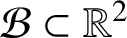
where the domain
 $\mathcal {B}\subset \mathbb {R}^2$
is the rectangle
 $[a,b] \times [c,d]$
, the kernel function
 $K(x,t,u(x,t))$
is continuous on
 $\mathcal {B} \times \mathbb {R}$
, and
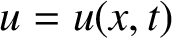
 $u(x,t)$
is an unknown function to be determined. The values of the solution
 $u = u(x, t)$
on the boundary are
 $$ \begin{align}\begin{aligned} u(x,c)&=g_1(x),\quad a\leq x\leq b, \\ u(a,t)&=g_2(t),\quad c\leq t\leq d, \end{aligned} \end{align} $$
in which the given real functions
 $g_1$
and
 $g_2$
are continuous and satisfy
 $g_1(a) = g_2(c)$
.
The Darboux problem, as a fundamental problem in mathematical physics, has been applied to simulate mathematical models in various areas such as condensed matter physics, fluid flow, nonlinear optics, radiation theory, solid and high-energy physics and quantum mechanics [Reference Chandhini, Prashanthi and Vijesh12]. The Darboux problem is known in the literature as the Goursat problem [Reference Lees28], and also can be considered as a limiting case of the Tricomi problem [Reference Chandhini, Prashanthi and Vijesh12]. Attempts to numerically solve these problems date back to 1960s. The Runge–Kutta type method [Reference Day14], the cubature method [Reference Jain and Sharma24] and the trapezoidal quadrature formula [Reference Gourlay23] were proposed for solving the Darboux problem. Later, nonlinear trapezoidal formulas based on geometric means [Reference Evans and Sanugi18] and harmonic means [Reference Wazwaz45] were also applied for the numerical solution of Goursat problems. A general class of difference schemes for this problem have been investigated by Czlapinski [Reference Czlapinski13]. The Runge–Kutta method and trapezoidal formula were used to solve these problems in a triangular domain with the mixed Dirichlet and impedance boundary conditions [Reference Gou and Sun22].
By integrating both sides of the Darboux problem (1.1), this equation can be reduced to the two-dimensional nonlinear Volterra integral equations [Reference Dobner17]. A few methods have been proposed for the approximate solution of the two-dimensional Volterra integral equations. Projection and iterated projection [Reference Atkinson6] are the commonly used approaches for the numerical solutions of two-dimensional integral equations. The collocation method [Reference Brunner and Kauthen10], the two-dimensional differential transform method [Reference Tari, Rahimi, Shahmorad and Talati43], the rationalized Haar functions [Reference Babolian, Bazm and Lima8], the geometric series theorem together with Schauder bases [Reference Berenguer and Gamez9] and the Legendre functions [Reference Nemati, Lima and Ordokhani38] were applied to obtain the numerical solution of the two-dimensional Volterra integral equations.
To apply projection methods for solving two-dimensional Volterra integral equations, the solution domain sometimes needs to be divided into nonoverlapping triangular fragments [Reference Atkinson6]. Therefore, to get rid of triangulations and mesh refinements, methods based upon the meshless scheme can be utilized which estimate a function without any mesh generation on the domain. Meshless discrete collocation schemes using radial basis functions (RBFs) were investigated for solving two-dimensional integral equations of the second kind with smooth kernels [Reference Assari, Adibi and Dehghan1] and weakly singular kernels [Reference Assari and Dehghan4]. RBFs were applied for the numerical solution of Volterra–Fredholm–Hammerstein integral equations [Reference Parand and Rad39] and singular-logarithmic boundary integral equations [Reference Assari and Dehghan5]. The meshless product integration method [Reference Assari, Adibi and Dehghan2] has been proposed to solve one-dimensional linear weakly singular integral equations. The moving least squares (MLS) collocation method was used for solving two-dimensional integral equations [Reference Mirzaei and Dehghan36]. An MLS-based Galerkin meshless method [Reference Li30, Reference Li and Li34] was utilized to solve the logarithmic boundary integral equations and an error estimate was obtained [Reference Li and Dong33].
In the past few decades, RBFs have been applied as an effective meshless technique for interpolating a function over a set of scattered points. Since the classical RBFs are global functions, the resultant coefficient matrix will be a full matrix, when many points in the domain are considered for obtaining high-order accurate results [Reference Wendland46]. Although this coefficient matrix is nonsingular, usually it is ill-conditioned, that is, a small perturbation in the initial data may produce a large perturbation in the solution [Reference Wendland46]. To overcome these difficulties, the advantages of RBFs with local supports could be utilized, which were investigated in the literature as local radial basis functions (LRBFs). To construct the approximation function with LRBFs, the only geometrical data needed are within the local influence domain. Therefore, LRBFs need much less computational work than globally supported RBFs, and eventually the interpolation matrix of LRBFs would be well-conditioned. Another additional benefit of this formulation is that we have much more freedom in choosing the shape parameter of the RBFs [Reference Sarler and Vertnik41].
A large number of papers have presented numerical schemes for solving several types of partial differential equations (PDEs) utilizing LRBFs. Such PDEs appear, for example, in diffusion-convection problems with phase change [Reference Vertnik and Sarler44], natural convection problems [Reference Kosec and Sarler26], natural convection under the influence of a static magnetic field [Reference Mramor, Vertnik and Sarler37], multi-dimensional convection-dominated problems [Reference Yun and Hon47], the system of second-order boundary value problems [Reference Dehghan and Nikpour16], polarized radiative transfer in participating media [Reference Sun, Yi and Tan42], thermoelasticity in two dimensions [Reference Mavric and Sarler35], convection-dominated fluid flow problems [Reference Yun and Hon47] and conservation laws equations [Reference Dehghan and Abbaszadeh15].
In the current investigation, we present a method for obtaining the numerical solution of the two-dimensional Darboux equation (1.1) with conditions (1.2). We first transform these types of equations into two-dimensional nonlinear Volterra integral equations of the second kind. Then, by combining the locally supported RBFs, the discrete Galerkin method is used to approximate the integral equations mentioned. In order to compute the integrals in the proposed method, we use the Gauss–Legendre integration rule [Reference Lether29] on the local influence domain. The new technique does not require any domain elements, so it is meshless. In comparison with the method based on globally supported RBFs for solving integral equations, the method presented in the current paper is well-conditioned and uses much less computer memory. Our scheme is simple, computationally attractive and more flexible. We also obtain the error bound and the convergence rate for the proposed method, and examine the convergence accuracy of the new approach in various Darboux equations.
The outline of the paper is as follows. In Section 2 we review some basic formulations and properties of the LRBF method. In Section 3 we present a computational method for solving the two-dimensional Darboux equation (1.1) by the LRBF scheme and provide the error analysis for the proposed method. We give numerical examples in Section 4. Section 5 concludes the paper.
2 Locally supported RBFs
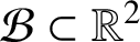
In this section locally supported RBFs are utilized to approximate a function on the domain
 $\mathcal {B}\subset \mathbb {R}^2$
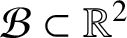
. Let
 $X=\{({x}_1,t_1),\ldots ,({x}_N,t_N)\}$
be a set of scattered points selected on the domain
 $\mathcal {B}\subset \mathbb {R}^2$
. We define the global interpolant
 $\mathcal {G}u$
of the function u at an arbitrary point
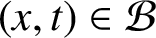 $(x,t) \in \mathcal {B}$
based on the radial function
 $$ \begin{align*}\Phi(x,t)=\phi ( \sqrt{x^2+t^2}).\end{align*} $$
Therefore, the function
 $\mathcal {G}u$
can be formulated by the linear combination [Reference Wendland46]
 $$ \begin{align} \mathcal{G}u(x,t)= \sum_{i=1}^Nc_i \Phi(x-x_i,t-t_i),\quad (x,t) \in \mathcal{B}. \end{align} $$
The function
 $\mathcal {G}u$
yields an interpolant that is translation invariant, that is, the interpolant to translated data is the same as the translated interpolant to the original data [Reference Fasshauer, Rieth and Schommers20]. To determine the values of the coefficients
 $\{c_1,\ldots ,c_{N}\}$
, one can evaluate the expansion (2.1) at all nodal points
 $(x_j,t_j)$
. Therefore, we have the interpolation conditions
 $$ \begin{align*} \mathcal{G}u(x_i,t_i) = u(x_i,t_i)=u_i,\quad i = 1,\ldots,N. \end{align*} $$
2.1 Interpolation by LRBFs
Suppose that
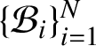 $\{\mathcal {B}_i\}_{i=1}^N$
is an open bounded cover for
 $\mathcal {B}$
, that is,
 $$ \begin{align*} \mathcal{B} \subseteq \bigcup_{i=1}^N\mathcal{B}_i, \end{align*} $$
where
 $\mathcal {B}_i$
is a subset of
 $\mathcal {B}$
centred at
 $({x}_i,t_i)$
with the radius
 $r_i$
. Let
 $I_i$
be the set of indexes corresponding to the points falling within the influence domain (or cover)
 $\mathcal {B}_i$
with cardinal number
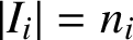 $|I_i|=n_{i}$
. The local interpolant
 $ \mathcal {L}_iu$
of the function u on the local support domain
 $\mathcal {B}_i$
based on the data sites
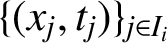 $\{({x}_j,t_j)\}_{j\in I_i} $
using a fixed RBF
 $\Phi $
can be considered as follows:
 $$ \begin{align} u({x},t)\approx \mathcal{L}_iu({x},t)=\sum_{j\in I_i} c_{j}^i \Phi(x-x_j,t-t_j),\quad (x,t) \in\mathcal{B}_i. \end{align} $$
In the expansion (2.2), the coefficients
 $\{c_j^i\}_{j \in I_i}$
are determined by enforcing the interpolation conditions
 $$ \begin{align} \mathcal{L}_iu({x}_k,t_k) = u_k,\quad k \in I_i,~i=1,\ldots,N. \end{align} $$
Therefore, we rewrite the interpolation problem (2.3) in the matrix form
 $$ \begin{align*} \mathbf{B}^i \mathbf{C}^i={\mathbf{U}}^i, \end{align*} $$
where
 $$ \begin{align*} {\mathbf{U}}^i&=[u_1,u_2,\ldots,u_{n_i}]^{T},\quad \mathbf{C}^i=[c_{1}^i,c_{2}^i,\ldots,c_{n_i}^i]^{T}, \\ \mathbf{B}^i&=[\Phi(x_k-x_j,t_k-t_j)],\quad k,j \in I_i. \end{align*} $$
Note that matrix
 $B^i$
is an
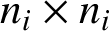 $n_i\times n_i$
real symmetric matrix and T denotes the transpose of a matrix.
Remark 2.1 [Reference Wendland46]
Note that if a radial basis function
 $\Phi $
is strictly positive definite then the associated interpolation matrix
 $\mathbf {B}^i$
is positive definite and so nonsingular. Therefore the interpolation problem (2.3) will be well-posed, that is, this problem has a unique solution.
Assume that
 $$ \begin{align*} \Lambda^i(x,t)=[\Phi(x-x_1,t-t_1), \Phi(x-x_2,t-t_2), \ldots , \Phi(x-x_{n_i},t-t_{n_i})]^{T}, \end{align*} $$
then the expansion (2.2) can be presented as
 $$ \begin{align} \mathcal{L}_iu ({x},t)=\Lambda^i({x},t)^{T}\mathbf{C}^i. \end{align} $$
Let the nodal points inside the cover
 $\mathcal {B}_{i}$
be distinct points. Then from Remark 2.1, we know that the matrix
 $\mathbf {B}^i$
is invertible, and so the column vector
 $\mathbf {C}^i$
is obtained by writing
 $$ \begin{align} \mathbf{C}^i=({\mathbf{B}^i})^{-1}{\mathbf{U}^i}. \end{align} $$
By substituting (2.5) in (2.4),
 $$ \begin{align*} \mathcal{L}_iu ({x},t)=\Lambda^i({x},t)^{T}({\mathbf{B}^i})^{-1}{\mathbf{U}^i}= \Psi^i({x},t)^{T}{\mathbf{U}^i}. \end{align*} $$
Therefore, we can represent the expansion (2.2) as [Reference Lee, Liu and Fan27]
 $$ \begin{align} \mathcal{L}_iu ({x},t)=\sum_{j \in I_i} u_j \psi^i_j({x},t), \end{align} $$
where
 $$ \begin{align*} \psi^i_j(x,t)= \sum_{k \in I_i} [({\mathbf{B}^i})^{-1}]_{kj}\Phi(x-x_k,t-t_k),\quad j \in I_i. \end{align*} $$
We explain the LRBF collocation method to approximate a function
 $u({x},t)$
at an arbitrary point
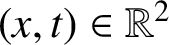 $(x,t) \in \mathbb {R}^2$
utilizing the RBF
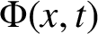 $\Phi ({x},t)$
by a linear combination as follows:
 $$ \begin{align} u(x,t)\approx \mathcal{Q}_Nu(x,t)= \sum_{i=1}^N u_i \psi^i_i({x},t),\quad (x,t) \in\mathcal{B}, \end{align} $$
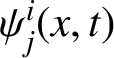
where the functions
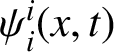 $\psi ^i_{i}(x,t)$
are called the shape functions for the LRBF interpolation.
The interpolation conditions (2.3) and the expansion (2.6) eventually result in the shape functions
 $\psi ^i_{j}({x},t)$
satisfying the Kronecker delta condition [Reference Lee, Liu and Fan27], and
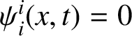 $\psi ^i_{i}(x,t)=0$
for every
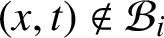 $(x,t) \notin \mathcal {B}_i$
. Therefore, many terms in the expansion (2.7) will vanish, namely,
 $$ \begin{align*} \mathcal{Q}_{N}u(x,t)=\sum_{i\in S_{(x,t)}} u_i \psi^i_i({x},t), \quad (x,t) \in \mathcal{B}, \end{align*} $$
where
 $S_{(x,t)}=\{i\mid {(x,t)}\in \mathcal {B}_i\}$
and the influence domain of the point
 $(x,t)$
is defined as
 $$ \begin{align*}\mathcal{B}_{(x,t)}=\bigcup_{i\in S_{(x,t)}}\mathcal{B}_i.\end{align*} $$
2.2 Error estimate for LRBFs
The real native Hilbert space with respect to the RBF
 $\Phi $
is defined as [Reference Wendland46]
 $$ \begin{align*} \aleph_{\Phi}(\Omega)=\left\{f \in C(\Omega) \cap L^2(\Omega) \Big|\, \frac{\hat{f}}{\sqrt{\hat{\Phi}}}\in L^2(\Omega)\right\}, \quad \Omega\subset \mathbb{R}^2 \end{align*} $$
with the inner product
 $$ \begin{align*} \langle f,g\rangle_{\aleph_{\Phi} (\Omega)}=\frac{1}{\sqrt{2\pi}}\bigg\langle\frac{\hat{f}}{\sqrt{\hat{\Phi}}},\frac{\hat{g}}{\sqrt{\hat{\Phi}}}\bigg\rangle_{L^2(\Omega)}= \frac{1}{\sqrt{2\pi}}\int_{\Omega} \frac{\hat{f}(w)\overline{\hat{g}(w)}}{\sqrt{\hat{\Phi}}}\,{d}w, \end{align*} $$
where
 $\hat {f}$
denotes the Fourier transform of f.
In the following, some definitions from [Reference Buhmann11, Reference Wendland46] are represented which are important for analysing the error of LRBF method.
Definition 2.2 [Reference Fasshauer, Rieth and Schommers20]
For a bounded domain
 $\Omega $
, the fill distance of a set of points
 $\mathcal {S} = \{(x_1,t_1), \ldots , (x_m,t_m)\}\subset \Omega \subset \mathbb {R}^2$
is defined by
 $$ \begin{align*}h_{\mathcal{S},\Omega}=\sup_{(x,t)\in \Omega} \min_{0\leq j \leq m}\sqrt{(x-x_j)^2+(t-t_j)^2}.\end{align*} $$
Definition 2.3 [Reference Fasshauer, Rieth and Schommers20]
The separation distance of
 $\mathcal {S} = \{(x_1,t_1), \ldots , (x_m,t_m)\}\subset D$
is defined by
 $$ \begin{align*}q_{\mathcal{S}}=\tfrac{1}{2}\min_{i\neq j}\sqrt{(x_i-x_j)^2+(t_i-t_j)^2}.\end{align*} $$
The set X is said to be quasi-uniform with respect to a constant
 $c> 0$
if
 $$ \begin{align*}q_{\mathcal{S}} \leq h_{\mathcal{S},\Omega} \leq cq_{\mathcal{S}}.\end{align*} $$
We are ready to give the convergence theorem for approximating a two-variable function by a strictly positive definite function [Reference Wendland46].
Theorem 2.4 [Reference Assari, Asadi-Mehregan and Dehghan3]
Suppose that
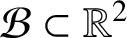 $\mathcal {B} \subset \mathbb {R}^2$
is a square domain and
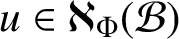 $u\in \aleph _{\Phi }(\mathcal {B})$
. If the derivatives of the strictly positive definite function
 $\Phi $
of order
 $2 \kappa $
are continuous on
 $\mathcal {B}$
, then there exist constants
 $\bar {h}_0,{C},{C}_{\Phi }> 0$
such that
 $$ \begin{align} |u(x,t)-\mathcal{Q}_{N}u(x,t)|\leq {C} C^{1/2}_{\Phi}\bar{h}_{\mathcal{B},X}^\kappa \|u\|_{\mathcal{B}}, \quad \bar{h}_{\mathcal{B},X} \leq \bar{h}_0, \end{align} $$
where
 $$ \begin{align*} \bar{h}_{\mathcal{B},X}=\max_{(x,t)\in\mathcal{B}}h_{\mathcal{B}_{(x,t)},S_{(x,t)}} \quad {and} \quad \|u\|_{\mathcal{B}} =\max_{(x,t)\in\mathcal{B}}\|u\|_{\aleph_{\phi}(\mathcal{B}_{(x,t)})}. \end{align*} $$
Remark 2.5 Theorem 2.4 for infinitely smooth functions
 $\Phi $
results in arbitrarily high algebraic convergence rates, that is, for every
 $l \in \mathbb {N}$
, we have [Reference Fasshauer, Rieth and Schommers20, Reference Wendland46]
 $$ \begin{align*} |u(x,t)-\mathcal{Q}_{N}u(x,t)|\leq {C}_{l}\bar{h}_{\mathcal{B},X}^l \|u\|_{\mathcal{B}},\quad \bar{h}_{\mathcal{B},X}\leq \bar{h}_0, \end{align*} $$
where the constant
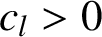 $c_l>0$
depends on l [Reference Fasshauer, Rieth and Schommers20].
For infinitely smooth strictly positive definite functions such as Gaussians and inverse multiquadrics, we present the following error bounds [Reference Wendland46].
-
(1) For Gaussians
 $\Phi (x,t) =e^{-c(x^2+t^2)},~c>0,$
we have
$$ \begin{align*} |u(x,t)-\mathcal{Q}_{N}u(x,t)| \leq e^{(-c|\ln \overline{h}_{\mathcal{B},X}|)/\bar{h}_{\mathcal{B},X}} \|u\|_{\mathcal{B}}. \end{align*} $$
-
(2) For inverse multiquadrics
$\Phi (x,t) = \sqrt {x^2+t^2 + c^2},~c> 0,$
we have
$$ \begin{align*} |u(x,t)-\mathcal{Q}_{N}u(x,t)| \leq e^{-c/\bar{h}_{\mathcal{B},X}} \|u\|_{\mathcal{B}}. \end{align*} $$




3 Solving Darboux equations
By integrating both sides of the Darboux equation (1.1) based on the use of conditions (1.2), this equation can be reduced to the following two-dimensional nonlinear Volterra integral equations:
 $$ \begin{align} u(x,t)-\int_a^x\int_c^t K(y,s,u(y,s))\,{d}y\,{d}s=g(x,t) , \quad (x,t)\in \mathcal{B}, \end{align} $$
where the nonhomogeneous term
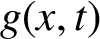 $g(x, t)$
contains the given initial values
 $$ \begin{align*} g(x,t)=g_1(x)+g_2(t)-g_1(a). \end{align*} $$
We can represent the integral equation (3.1) in operator form
 $$ \begin{align} \mathcal{H} u= u, \end{align} $$
where the Volterra integral operator
 $\mathcal {H}:L^2(\mathcal {B})\rightarrow L^2(\mathcal {B})$
is given by
 $$ \begin{align*} \mathcal{H}u = g + \mathcal{K} u=g(x,t)+\int_a^x\int_c^t K(y,s, u(y,s)) \,{d}s\, {d}y, \quad (x,t)\in \mathcal{B}, \end{align*} $$
with the integral operator
 $\mathcal {K}:L^2(\mathcal {B})\rightarrow L^2(\mathcal {B})$
defined as
 $$ \begin{align*}\mathcal{K} u(x,t)=\int_a^x\int_c^t K(y,s, u(y,s)) \,{d}s\,{d}y, \quad (x,t)\in \mathcal{B}.\end{align*} $$
Therefore, solving the integral equation (3.1) is equivalent to obtaining the fixed points of the operator
 $\mathcal {H}$
. To solve the integral equation (3.1), let
 $X=\{({x}_1,t_1),\ldots ,({x}_N,t_N)\}$
be N nodal points randomly selected on the domain
 $\mathcal {B}$
and
 $$ \begin{align*}\mathcal{B}_{i}=\{(x,t)\mid x_i-r_i \leq x \leq x_i+r_i,~~ t_i-r_i \leq t \leq t_i+r_i \}, \quad i=1,\ldots,N,\end{align*} $$
in which
 $r_i>0$
is chosen such that
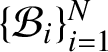 $\{\mathcal {B}_{i}\}_{i=1}^N$
is an open bounded cover for the rectangle
 $\mathcal {B}$
.
We estimate the unknown function
 $u(x,t)$
by the LRBF approximation as follows:
 $$ \begin{align} u(x,t)\approx \bar{u}_N(x,t)=\sum_{i=1}^N \bar{c}_i\psi_i^i(x,t), \quad (x,t)\in \mathcal{B}, \end{align} $$
where
 $\{\psi _1^1(x,t),\ldots ,\psi _N^N(x,t)\}$
are the shape functions of the LRBF method corresponding to the set X, and the coefficients
 $\{\bar {c}_1,\ldots ,\bar {c}_N\}$
are found by solving the system (3.4).
We assume
 $\langle \cdot ,\cdot \rangle $
is the inner product on
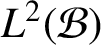 $L^2(\mathcal {B})$
, that is,
 $$ \begin{align*} \langle f,g\rangle =\int_a^b \int_c^d f(x,t)g(x,t)\,{d}x\, {d}t, \quad f,g\in L^2(\mathcal{B}). \end{align*} $$
By replacing the expansion (3.3) in the integral equation (3.1) instead of
 $u(x,t)$
, and taking the inner product
 $\langle \cdot ,\psi _j^j\rangle $
on both sides,
 $$ \begin{align*} \langle \bar{u}_N ,\psi_j^j \rangle = \langle g, \psi_j^j \rangle + \langle \mathcal{K} \bar{u}_N, \psi_j^j \rangle, \end{align*} $$
or equivalently,
 $$ \begin{align} \sum_{i=1}^N \bar{c}_i &\int_{\mathcal{B}} \psi_i^i(x,t) \psi_j^j(x,t)\, {d}x\, {d}t - \int_{\mathcal{B}} \int_a^x\int_c^t K\bigg(y,s,\sum_{i=1}^N \bar{c}_i \psi_i^i(y,s)\bigg) \psi_j^j(x,t) \,{d}y\, {d}s\, {d}x\, {d}t \nonumber\\ &= \int_{\mathcal{B}} \psi_j^j(x,t) g(x,t)\, {d}x\, {d}t. \end{align} $$
Since the support of the shape functions
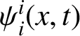 $\psi _{i}^{i}(x,t)$
is
 $$ \begin{align*}\mathcal{B}_i=[x_i-r_i,x_i+r_i]\times[t_i-r_i,t_i+r_i],\end{align*} $$
we have
 $$ \begin{align} &\sum_{i=1}^N \bar{c}_i \int_{\mathcal{B}\cap\mathcal{B}_{i}\cap\mathcal{B}_{j}} \psi_i^i(x,t) \psi_j^j(x,t)\,{d}x\, {d}t \nonumber\\ &\quad\quad -\int_{\mathcal{B}\cap\mathcal{B}_j} \int_a^x\int_c^t K\bigg(y,s,\sum_{i=1}^N \bar{c}_i \psi_i^i(y,s) \bigg)\psi_j^j(x,t) \, {d}y \,{d}s\, {d}x\, {d}t \nonumber\\ &\quad= \int_{\mathcal{B}\cap\mathcal{B}_j} \psi_j^j(x,t) g(x,t)\, {d}x \,{d}t. \end{align} $$
For a general function
 $u({x})\in L^2[a,b]$
, we define the Galerkin operator
 $\mathcal {S}_{N}$
[Reference Atkinson6] to be a solution of the minimization problem
 $$ \begin{align*} \|u- \mathcal{S}_{N}u\|=\min_{z \in V_N(\mathcal{B})}\|u-z\|, \end{align*} $$
where
 $V_N(\mathcal {B})=\mathrm {span}\{\psi _1^1,\ldots ,\psi _N^N\}$
is a subspace of the space
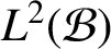 $L^2(\mathcal {B})$
. Note that since
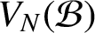 $V_N(\mathcal {B})$
is finite-dimensional, this problem has a solution; and since it is also an inner product space, the solution
 $$ \begin{align*} \mathcal{S}_{N}u(x,t)=\sum_{i=1}^N {c}_i\psi_i^i(x,t),\quad (x,t)\in \mathcal{B}, \end{align*} $$
is unique [Reference Atkinson6], where the coefficients
 $\{c_1,\ldots ,c_N\}$
are determined by solving the linear system
 $$ \begin{align*} \langle u,\psi_j^j \rangle = \sum_{i=1}^N {c}_i \langle \psi_i^i,\psi_j^j \rangle, \quad j=1,\ldots ,N. \end{align*} $$
The discrete Galerkin methods result from the numerical integration of all integrals in the system (3.5) associated with the Galerkin method. There are two types of integrals to be evaluated in this system:
-
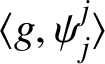
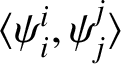
(1) the double integrals
$\langle g,\psi _j^j\rangle $
and
$\langle \psi _i^i,\psi _j^j \rangle $
; -
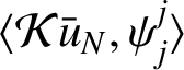
(2) the quadruple integrals
$\langle \mathcal {K}\bar {u}_N,\psi _j^j \rangle $
.
We estimate these integrals utilizing the m-point Gauss–Legendre rule [Reference Lether29] on the interval
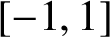 $[-1,1]$
. Suppose that
 $P_m(x)$
, is the well-known Legendre polynomial of order m with roots
 $v_k,~k=1,\ldots ,m,$
and
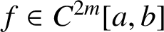 $f\in C^{2m}[a,b]$
. Then
 $$ \begin{align} \int_{a}^{b} f(x)\,{d}x \approx \frac{b-a}{2} \sum_{k=1}^{m}w_k f (\theta_{k}), \end{align} $$
where
 $$ \begin{align*} w_k=\frac{2}{(k+1)P'_{m+1}(v_k)P_m(v_k)}\quad \mathrm{and} \quad \theta_{k}=\frac{1}{2} [a+b+(b-a)v_k]. \end{align*} $$
It can be proved that [Reference Quarteroni, Sacco and Saleri40]
 $$ \begin{align*} \bigg|\int_{a}^{b} f(x) \,{d}x - \frac{b-a}{2} \sum_{k=1}^{m}w_k f (\theta_{k}) \bigg| \leq \frac{2^{2m}{(b-a)}^{2m+1}}{(2m)!}\max_{a\leq x \leq b}|\,f^{(2m)}(x)|. \end{align*} $$
Using the m-point Gauss–Legendre quadrature rule relative to the coefficients
 $\{v_{k}\}$
and weights
 $\{w_{k}\}$
in the interval
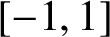 $[-1,1]$
, we define a discrete semidefinite inner product
 $$ \begin{align*} \langle f,g \rangle \approx \langle f,g \rangle_N=\frac{(b-a)(d-c)}{4} \sum_{k=1}^{m}w_k \sum_{q=1}^m f(\theta_k,\eta_{q}) g(\theta_k,\eta_{q}),\quad f,g\in L^2(\mathcal{B}), \end{align*} $$
where
 $\theta _k=[a+b+(b-a)v_k]/2$
and
 $\eta _{q}=[c+d+(d-c)v_q]/2$
.
We now define the discrete Galerkin operator
 $\mathcal {G}_{N}:L^2(\mathcal {B})\rightarrow L^2(\mathcal {B})$
:
 $$ \begin{align*} \mathcal{G}_{N}u(x,t)=\sum_{k=1}^Nc_k\psi_k^k(x,t),\quad (x,t)\in \mathcal{B}, \end{align*} $$
with coefficients
 $\{c_1,\ldots ,c_N\}$
determined by solving the linear system
 $$ \begin{align*} \langle u,\psi_j^j \rangle_{N}=\sum_{k=1}^Nc_k \langle \psi_k^k,\psi_j^j \rangle_{N},\quad j=1,\ldots ,N. \end{align*} $$
Let the family
 $\{\mathcal {G}_N \mid N \geq 1\}$
be uniformly bounded on
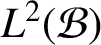 $L^2(\mathcal {B})$
, say,
 $$ \begin{align} \|\mathcal{G}_N\|\leq m. \end{align} $$
Then we have [Reference Atkinson6]
 $$ \begin{align*} \|\mathcal{G}_Nu-u\| \leq (1+m) \|\mathcal{S}_Nu-u\|. \end{align*} $$
Remark 3.1 The proof of uniform boundedness for the operators
 $\{\mathcal {Q}_N\}$
was investigated at some length by Atkinson and Bogomolny [Reference Atkinson and Bogomolny7].
In order to apply the quadrature formula (3.6) for computing the double integrals
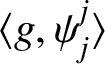 $\langle g,\psi _j^j\rangle $
, we first consider
 $$ \begin{align} \langle g,\psi_j^j\rangle = \int_{\mathcal{B}\cap\mathcal{B}_j} \psi_j^j(x,t) g(x,t) \,{d}x \, {d}t = \int_{\alpha_j}^{\beta_j}\bigg( \int_{\gamma_j}^{\delta_j} \psi_j^j(x,t) g(x,t) \,{d}t \bigg)\,{d}x, \end{align} $$
where
 $$ \begin{align*} \alpha_j&=\max\{a,x_j-r_j\},\quad \beta_j=\min\{b,x_j+r_j\},\\ \gamma_j&=\max\{c,t_j-r_j\},\quad \delta_j=\min\{d,t_j+r_j\}. \end{align*} $$
Since the weight functions used in the current work are several times continuously differentiable on
 $\mathcal {B}$
, the shape functions
 $\psi _j^j$
and g are in
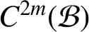 $C^{2m}(\mathcal {B})$
for every
 $m\in \mathbb {N}$
. Therefore, we can estimate the external integral on the right-hand side of (3.8) by
 $$ \begin{align*} \langle g,\psi_j^j\rangle \approx \frac{\beta_{j}-\alpha_{j}}{2} \sum_{k=1}^{m}w_k \bigg( \int_{\gamma_{j}}^{\delta_{j}} \psi_i^i(\theta_{k,j},t) \psi_j^j(\theta_{k,j},t) \, {d}t \bigg), \end{align*} $$
where
 $\theta _{k,j}=[\alpha _j+\beta _j+(\beta _j-\alpha _j)v_k]/2$
. Again by replicating this scheme for internal integrals, we have
 $$ \begin{align} \langle g,\psi_j^j\rangle \approx \frac{(\delta_{j}-\gamma_{j})(\beta_{j}-\alpha_{j})}{4} \sum_{k=1}^{m }w_k \sum_{q=1}^mw_q g(\theta_{k,j},\eta_{q,j}) \psi_j^j(\theta_{k,j},\eta_{q,j}), \end{align} $$
where
 $\eta _{q,j}=[\gamma _j+\delta _j+(\delta _j-\gamma _j)v_q]/2$
.
Similarly, based on the use of the quadrature rule (3.6), we estimate the double integral
 $$ \begin{align*} \langle \psi_i^i,\psi_j^j\rangle = \int_{\mathcal{B}\cap\mathcal{B}_{i}\cap\mathcal{B}_{j}} \psi_i^i(x,t) \psi_j^j(x,t) \,{d}x \,{d}t=\int_{\alpha_{ij}}^{\beta_{ij}}\int_{\gamma_{ij}}^{\delta_{ij}} \psi_i^i(x,t) \psi_j^j(x,t) \,{d}x \,{d}t, \end{align*} $$
where
 $$ \begin{align*} \alpha_{ij}&=\max\{\alpha_i,\alpha_j\},\quad \beta_{ij}=\min\{\beta_i,\beta_j\},\\ \gamma_{ij}&=\max\{\gamma_i,\gamma_j\},\quad \delta_{ij}=\min\{\delta_i,\delta_j\}. \end{align*} $$
Therefore,
 $$ \begin{align} \langle \psi_i^i,\psi_j^j\rangle \approx \frac{(\delta_{ij}-\gamma_{ij})(\beta_{ij}-\alpha_{ij})}{4} \sum_{k=1}^{m}w_k \sum_{q=1}^m w_q\psi_i^i(\theta_{k,ij},\eta_{q,ij}) \psi_j^j(\theta_{k,ij},\eta_{q,ij}), \end{align} $$
where
 $\theta _{k,ij}=[\alpha _{ij}+\beta _{ij}+(\beta _{ij}-\alpha _{ij})v_k]/2$
and
 $\eta _{q,ij}=[\gamma _{ij}+\delta _{ij}+(\delta _{ij}-\gamma _{ij})v_q]/2$
.
We compute the quadruple integral as
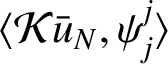 $\langle \mathcal {K}\bar {u}_N,\psi _j^j\rangle $
:
 $$ \begin{align*} \langle \mathcal{K}\bar{u}_N,\psi_j^j \rangle = \int_{\alpha_j}^{\beta_j}\int_{\gamma_j}^{\delta_{j}} \bigg[\int_a^x\int_c^t K\bigg(y,s,\sum_{i=1}^N \bar{c}_i \psi_i^i(y,s)\bigg) \psi_j^j(x,t) \, {d}s \,{d}y \bigg]\,{d}x\, {d}t. \end{align*} $$
Now utilizing a process similar to the quadrature rule (3.6) for approximating the double integral on
 $\mathcal {B}$
, it is concluded that
 $$ \begin{align*} \langle \mathcal{K}\bar{u}_N,\psi_j^j \rangle \approx\frac{(\delta_{j}-\gamma_{j})(\beta_{j}-\alpha_{j})}{4} \sum_{k=1}^{m}w_k \sum_{q=1}^mw_q G[j,\theta_{k,j},\eta_{q,j},\bar{c}_1,\ldots.\bar{c}_N], \end{align*} $$
where
 $$ \begin{align} G[j,\theta_{k,j},\eta_{q,j},\bar{c}_1,\ldots ,\bar{c}_N]=\int_a^{\theta_{k,j}}\int_c^{\eta_{q,j}} K\bigg(y,s,\sum_{i=1}^N \bar{c}_i \psi_i^i(y,s) \bigg)\psi_j^j(\theta_{k,j},\eta_{q,j}) \, {d}s\, {d}y. \end{align} $$
In the following, we apply the quadrature rule (3.6) for computing the external integral of (3.11) as
 $$ \begin{align*} &G[j,\theta_{k,j},\eta_{q,j},\bar{c}_1,\ldots ,\bar{c}_N] \nonumber \\ &\quad\approx\frac{\theta_{k,j}-a}{2} \sum_{r=1}^{m}w_r \int_c^{\eta_{q,j}} K\bigg(\tau_{r,j}(\theta_{k,j}),s,\sum_{i=1}^N \bar{c}_i \psi_i^i(\tau_{r,j}(\theta_{k,j}),s)\bigg) \psi_j^j(\theta_{k,j},\eta_{q,j}) \, {d}s, \end{align*} $$
where
 $\tau _{r,j}(\theta _{k,j})=[a+\theta _{k,j}+(\theta _{k,j}-a)v_r]/2$
.
To complete the integration scheme for approximating the integral
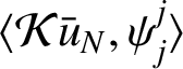 $\langle \mathcal {K}\bar {u}_N,\psi _j^j\rangle $
, we use the quadrature rule (3.6) for the internal integral of (3.11). This yields
 $$ \begin{align} \langle \mathcal{K}\bar{u}_N,\psi_j^j\rangle \approx \frac{(\delta_{j}-\gamma_{j})(\beta_{j}-\alpha_{j})}{4} \sum_{k=1}^{m}w_k \sum_{q=1}^mw_q \mathcal{I}[j,\tau_{r,j}(\theta_{k,j}),\rho_{p,j}(\eta_{q,j}),\bar{c}_1,\ldots ,\bar{c}_N], \end{align} $$
where
 $$ \begin{align*} &\mathcal{I}[j,\tau_{r,j}(\theta_{k,j}),\rho_{p,j}(\eta_{q,j}),\bar{c}_1,\ldots \bar{c}_N] =\frac{(\eta_{q,j}-c)(\theta_{k,j}-a)}{4}\nonumber\\ &\quad \times \sum_{r=1}^{m}w_r \sum_{p=1}^m w_{p} K\bigg(\tau_{r,j}(\theta_{k,j}),\rho_{p,j}(\eta_{q,j}),\sum_{i=1}^N \bar{c}_i \psi_i^i(\tau_{r,j}(\theta_{k,j}),\rho_{p,j}(\eta_{q,j}))\bigg) \psi_j^j(\theta_{k,j},\eta_{q,j}), \end{align*} $$
with
 $\rho _{p,j}(\eta _{q,j})=[c+\eta _{q,j}+(\eta _{q,j}-c)v_p]/2$
.
Utilizing the numerical integration schemes (3.9), (3.10) and (3.12) in the system (3.4) yields the linear system of algebraic equations
 $$ \begin{align} &\sum_{i=1}^N \hat{c}_i \frac{(\delta_{ij}-\gamma_{ij})(\beta_{ij}-\alpha_{ij})}{4} \sum_{k=1}^{m}w_k \sum_{q=1}^m w_q\psi_i^i(\theta_{k,ij},\eta_{q,ij}) \psi_j^j(\theta_{k,ij},\eta_{q,ij}). \nonumber\\ &\quad\quad -\frac{(\delta_{j}-\gamma_{j})(\beta_{j}-\alpha_{j})}{4} \sum_{k=1}^{m}w_k \sum_{q=1}^m w_q \mathcal{I}[j,\tau_{r,j}(\theta_{k,j}),\rho_{p,j}(\eta_{q,j}),\hat{c}_1,\ldots ,\hat{c}_N] \nonumber\\ &\quad =\frac{(\delta_{j}-\gamma_{j})(\beta_{j}-\alpha_{j})}{4} \sum_{k=1}^{m }w_k \sum_{q=1}^mw_q g(\theta_{k,j},\eta_{q,j}) \psi_j^j(\theta_{k,j},\eta_{q,j}). \end{align} $$
Based on the m-point Gauss–Legendre quadrature rule relative to the coefficients
 $\{v_{k}\}$
and weights
 $\{w_{k}\}$
in the interval
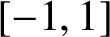 $[-1,1]$
, a sequence of numerical integral operators
 $\mathcal {H}_{N}$
on
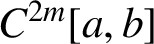 $C^{2m}[a,b]$
is defined by
 $$ \begin{align*} \mathcal{H}_Nu(x,t)=g(x,t)+ \lambda\frac{(x-a)(t-c)}{4} \sum_{r=1}^{m}w_r \sum_{p=1}^{m}w_p K(\tau_r(x),\rho_{p}(t),u(\tau_r(x),\rho_{p}(t))), \end{align*} $$
where
 $\tau _r(x)=[a+x+(x-a)v_r]/2$
and
 $\rho _{p}(t)=[c+t+(t-c)v_p]/2.$
Note that
 $\{\mathcal {H}_N\}$
is a collectively compact set and converges pointwise [Reference Fang, Wang and Xu19, Reference Kaneko and Xu25]. Moreover, for every
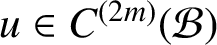 $u \in C^{(2m)}(\mathcal {B})$
and
 $K \in C^{(2m)}(\mathcal {B} \times \mathcal {B})$
, we have [Reference Fang, Wang and Xu19]
 $$ \begin{align} \|\mathcal{H}u-\mathcal{H}_Nu\|\leq \mathcal{C}_{m} \frac{\gamma_{\mathcal{B}}^{2m+1}}{2(2m)!}, \end{align} $$
where
 $\gamma _{\mathcal {B}}=(x-a)(t-c)$
.
We can represent the final system (3.13) in the abstract form
 $$ \begin{align} \mathcal{G}_N\mathcal{H}_N \hat{u}_N= \hat{u}_N, \end{align} $$
where the solution
 $\hat {u}_N$
is obtained by the proposed scheme in the current paper. The solution of this system for the unknowns
 $\{\hat {c}_1, \ldots , \hat {c}_N \}$
eventually leads to the following numerical solution which can approximate
 $u(x,t)$
as
 $$ \begin{align*} \hat{u}_N(x,t)=\sum_{i=1}^N \hat{c}_i\psi_i^i(x,t),\quad (x,t)\in \mathcal{B}. \end{align*} $$
Remark 3.2 The proposed meshless method in the current paper is applied to the two-dimensional Darboux problem. We note that applications of other meshless methods such as the finite-point method [Reference Li and Zhu31], the point interpolation method [Reference Li and Zhu32] and the element-free Galerkin method [Reference Zhang and Li49, Reference Zhang, Lin and Rao50] can be considered to extend of the proposed method to higher dimensions in the future.
The mean-value theorem for the kernel function
 $k(y,s,u(y,s))$
implies that there exists a function
 $\xi (x,t)$
, whose value
 $\xi (x,t)$
is between
 $u(x,t)$
and
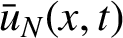 $\bar {u}_N(x,t)$
, such that
 $$ \begin{align} K(y,s,u(y,s))-K(y,s,\hat{u}_N(y,s))=K_u(y,s,\xi(y,s))\hat{e}_N(y,s), \end{align} $$
where
 $\hat {e}_N=u-\hat {u}_N$
. We define the operators
 $\mathcal {H}'$
and
 $\mathcal {H}''$
from
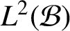 $L^2(\mathcal {B})$
to
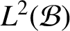 $L^2(\mathcal {B})$
as follows:
 $$ \begin{align} \mathcal{H}'\phi(x,t)=\frac{(b-a)(d-c)}{4} \sum_{k=1}^{m}w_k \sum_{q=1}^m K_u(\theta_k,\eta_{q},u(\theta_k,\eta_{q}))\phi(\theta_k,\eta_{q}) \end{align} $$
and
 $$ \begin{align} \mathcal{H}''\phi(x,t)=\frac{(b-a)(d-c)}{4} \sum_{k=1}^{m}w_k \sum_{q=1}^m K_u(\theta_k,\eta_{q},\xi(\theta_k,\eta_{q}))\phi(\theta_k,\eta_{q}), \end{align} $$
where
 $\theta _k=[a+b+(b-a)v_k]/2$
and
 $\eta _{q}=[c+d+(d-c)v_q]/2$
.
Throughout this paper, we resort to the standard hypothesis, such that
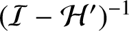 $(\mathcal {I}-\mathcal {H}')^{-1}$
always exists and is bounded [Reference Zhang and Li48]. Based on the above assumptions, as
 $N\rightarrow \infty $
, we have [Reference Zhang and Li48]
 $$ \begin{align} \|\mathcal{H}' - \mathcal{H}''\|\rightarrow 0\quad\mathrm{and}\quad \|(\mathcal{I}-\mathcal{G}_N)\mathcal{H}'\|\rightarrow 0. \end{align} $$
From (3.2), we obtain
 $$ \begin{align*} \mathcal{G}_Nu=\mathcal{G}_N\mathcal{H}u. \end{align*} $$
Now using (3.15) leads to
 $$ \begin{align*} \mathcal{G}_Nu-\hat{u}_N =\mathcal{G}_N [\{\mathcal{H}u-\mathcal{H}_Nu\}+\{\mathcal{H}_Nu-\mathcal{H}_N\hat{u}_N\}]. \end{align*} $$
Based on the use of (3.16), we have
 $$ \begin{align*} \mathcal{H}_Nu-\mathcal{H}_N\hat{u}_N= \mathcal{H}'' \hat{e}_N =\mathcal{H}'' (u-\hat{u}_N). \end{align*} $$
Therefore, we conclude that
 $$ \begin{align*} (\mathcal{I}-\mathcal{G}_N\mathcal{H}'')\hat{e}_N=\mathcal{G}_N(\mathcal{H}u-\mathcal{H}_Nu)+(\mathcal{G}_Nu-u). \end{align*} $$
To show the existence of the inverse operator
 $(\mathcal {I}-\mathcal {G}_N\mathcal {H}'')^{-1}$
, similar to [Reference Zhang and Li48], we consider
 $$ \begin{align*} \mathcal{I}-\mathcal{G}_N\mathcal{H}''&=(\mathcal{I}-\mathcal{G}_N\mathcal{H}')+\mathcal{G}_N(\mathcal{H}'-\mathcal{H}'')\nonumber\\ &=(\mathcal{I}-\mathcal{H}')+(\mathcal{I}-\mathcal{G}_N)\mathcal{H}'+\mathcal{G}_N(\mathcal{H}'-\mathcal{H}'')\nonumber\\ &= (\mathcal{I}-\mathcal{H}') [\mathcal{I}+(\mathcal{I}-\mathcal{H}')^{-1} \{(\mathcal{I}-\mathcal{G}_N)\mathcal{H}'+\mathcal{G}_N(\mathcal{H}' -\mathcal{H}'') \} ]. \end{align*} $$
The existence and uniform boundedness of
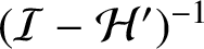 $(\mathcal {I}-\mathcal {H}')^{-1}$
and the use of (3.19) imply that the operator
 $(\mathcal {I}-\mathcal {G}_N\mathcal {H}'')^{-1}$
exists and is uniformly bounded for sufficiently large N, that is,
 $$ \begin{align*}\|(\mathcal{I}-\mathcal{G}_N\mathcal{H}'')^{-1}\|\leq \eta,\end{align*} $$
where
 $\eta $
is a positive constant. Therefore,
 $$ \begin{align*} \|\hat{e}_N\| \leq \|(\mathcal{I}-\mathcal{Q}_N\mathcal{H}'')^{-1}\|\,\|\mathcal{Q}_N\|[\,\|\mathcal{H}u-\mathcal{H}_Nu\|+\|\mathcal{Q}_Nu-u\|\,]. \end{align*} $$
Finally, from error bounds (2.8) and (3.14) and the uniform boundedness of the family
 $\{\mathcal {Q}_N\}$
in (3.7) we have
 $$ \begin{align} \|u-\hat{u}_N\| \leq \eta m\bigg[ \mathcal{C}_{m} \frac{\gamma_{\mathcal{B}}^{2m+1}}{2(2m)!}+{C} {C}^{1/2}_{\Phi}\bar{h}_{\mathcal{B},X}^\kappa \|u\|_{\mathcal{B}} \bigg]. \end{align} $$
Remark 3.3 The error bound (3.20) shows that the error of the scheme presented in the current paper is mainly based upon the LRBF interpolation error and the error caused by applying the m-point Gauss–Legendre quadrature rule. We conclude that for sufficiently large m, the LRBF interpolation error is dominated over by the integration error. In this situation, increasing the number of nodes in numerical integration has no significant effect on the error, and the approximation order of the proposed method will be
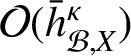 $\mathcal {O}(\bar {h}_{\mathcal {B},X}^\kappa )$
.
4 Numerical examples
In order to demonstrate the efficiency and accuracy of the proposed method, we solve some Darboux problems. For the tests, we used local Gaussian (LGAs) and local inverse multiquadrics (LIMQs) in the scheme. Since LRBFs have much more freedom in choosing the shape parameters, we select
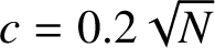 $c=0.2\sqrt {N}$
for LGAs and
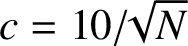 $c=10/\kern-3pt\sqrt {N}$
[Reference Fasshauer and Zhang21]. The cover size
 $r_i$
of the node
 $(x_i,t_i)$
is determined as follows [Reference Lee, Liu and Fan27].
-
(1) Consider the four nearest the nodes
$(x_j,t_j),~j=1,2,3,4$
to
$({x}_i,t_i)$
. -
(2) Define
$$ \begin{align*}d_i=\max_{j=1,2,3,4}\sqrt{({x}_i-{x}_j)^2-(t_i-t_j)^2}.\end{align*} $$
-
(3) Determine the cover size
$r_i$
of
$({x}_i,t_i)$
such that
$r_i=2 d_i.$



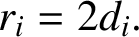
As a result of this selection of the cover size there are not too many nodes falling within a nodal cover in the densely populated zone, or too few falling within a nodal cover in the sparsely populated zone [Reference Lee, Liu and Fan27]. Based on the discussion in Remark 3.3, we compute the integrals appearing in the scheme, using Gauss–Legendre quadrature rule with
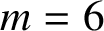 $m=6$
. Since the Gaussian and inverse multiquadrics applied in the illustrative examples are infinitely smooth strictly positive definite functions, the proposed method will yield arbitrarily high algebraic convergence orders.
We have measured the accuracy of our technique by the maximum error
 $\|e_N\|_{\infty }$
and the mean error
 $\|e_N\|_2$
which are defined as
 $$ \begin{align*}\|e_N\|_{\infty}=\max_{(x,t) \in \mathcal{B}}\{|u_{\mathrm{ex}}({x},t)-\hat{u}_{N}({x},t)|\}, \quad \|e_N\|_2=\bigg(\int_{\mathcal{B}} |u_{\mathrm{ex}}({x},t)-\hat{u}_{N}({x},t)|^2 \,{d}x \, {d}t \bigg)^{1/2},\end{align*} $$
where the exact solution
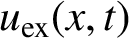 $u_{\mathrm {ex}}(x,t)$
is estimated by the numerical solution
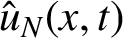 $\hat {u}_{N}(x,t)$
obtained in the current paper. The convergence rate of the scheme presented is also reported as
 $$ \begin{align*}\text{Ratio} =\frac{\ln(\|e_{N}\|_{\infty})-\ln(\|e_{N'}\|_{\infty})}{\ln(\bar{h}^{'}_X)-\ln(\bar{h}^{}_X)}.\end{align*} $$
We have written all routines in MAPLE software with the 20 “Digits” option (the Digits environment variable controls the number of digits in MAPLE) and a laptop with 2.10 GHz Intel® CoreTM 2 CPU and 4 GB of RAM has been used to run these. To solve the final nonlinear system of algebraic equations the Fsolve command has been employed based on the use of floating-point arithmetic.
Example 4.1 Consider the two-dimensional Darboux equation
 $$ \begin{align} u_{xt}=\tfrac{3}{4}(3t+2x)(3t^2+3x)u^5(x,t)-2u^3(x,t), \quad (x,t)\in [0,\pi/2] \times [0,2], \end{align} $$
with conditions
 $$ \begin{align*} \begin{array}{ll} u(x,0)=\dfrac{1}{\sqrt{x^2+6}},&\quad 0\leq x\leq \pi/2,\\[9pt] u(0,t)=\dfrac{1}{\sqrt{t^3+6}},&\quad 0\leq t\leq 2, \end{array} \end{align*} $$
and exact solution
 $u_{\mathrm {ex}}=1/\sqrt {x^2+t^3+xt+6}.$
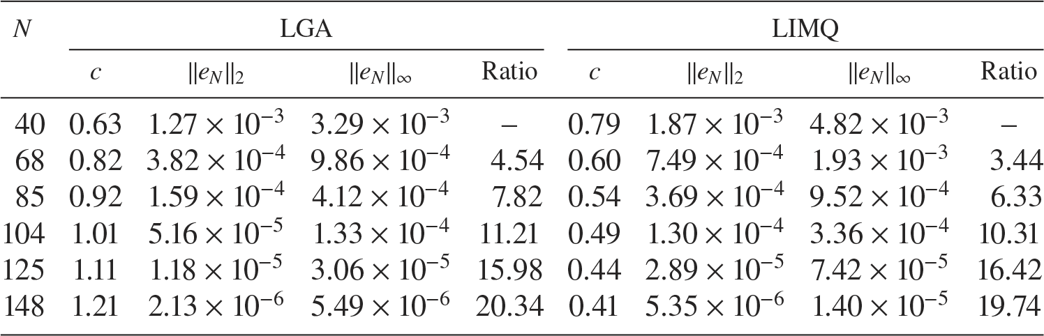
Table 1 reports
 $\|e\|_{\infty }$
,
 $\|e\|_2$
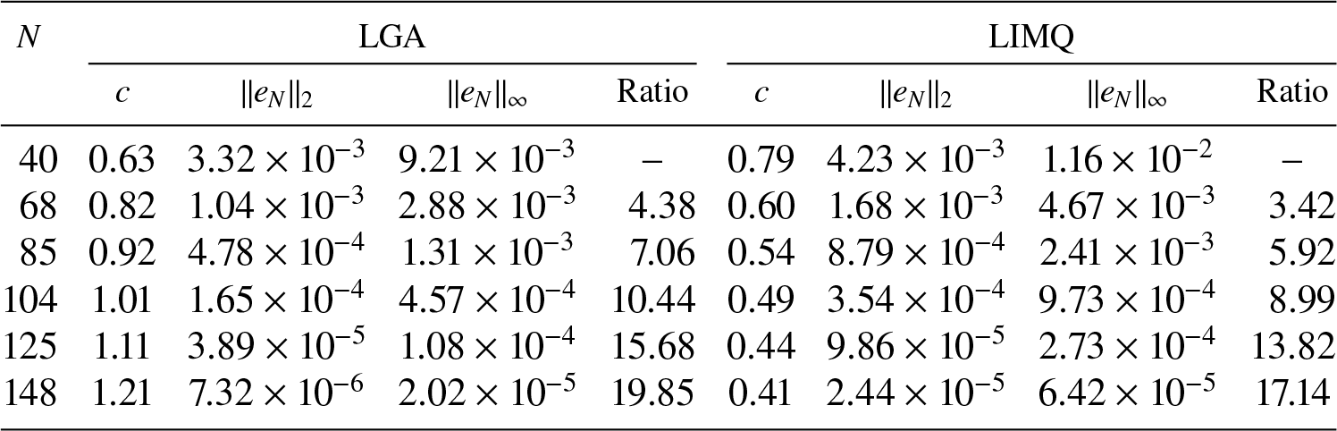
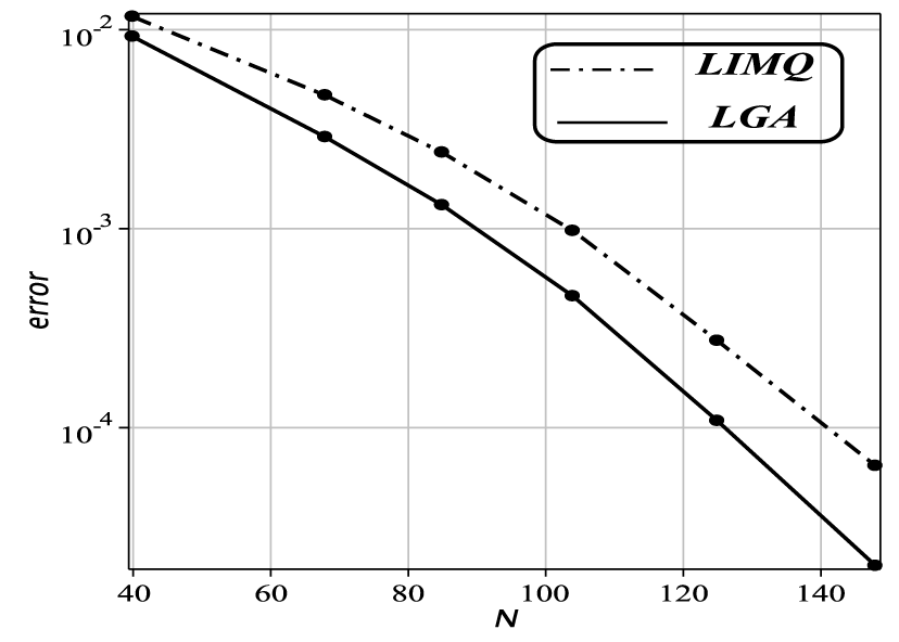
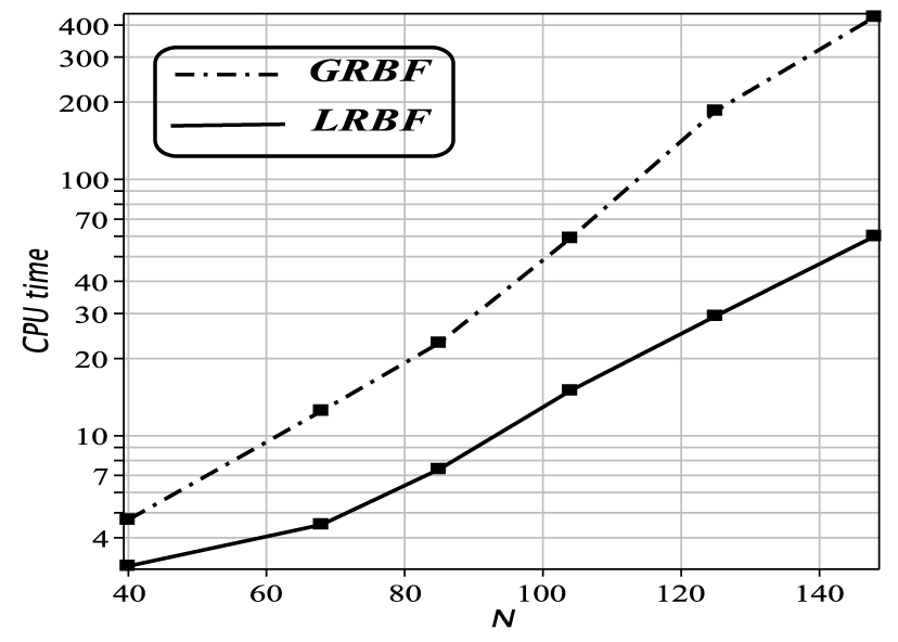
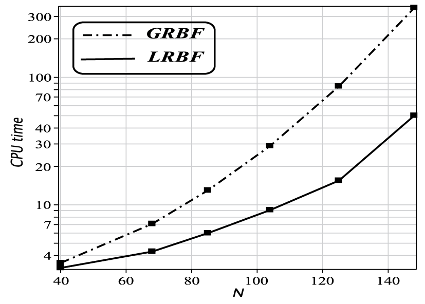
and the values of the ratio at different numbers of N. The errors obtained for different values of N are drawn on a logarithmic scale in Figure 1. We have also compared the CPU times for solving the Darboux equation (4.1) using global and local RBF for different N in Figure 2. It is worth pointing out that the CPU times of the proposed method are much lower than the global RBFs, which confirms that the new approach is very fast. From the error bound (3.20), we know that the results gradually converge to the exact values as the number of nodes increases with arbitrarily high order, because these LRBFs are several times continuously differentiable.
Some numerical results for Example 4.1 using the proposed method.

Distribution of absolute error for Example 4.1.

CPU times for Example 4.1.

Example 4.2 Consider the two-dimensional Darboux equation
 $$ \begin{align*} u_{xt}=\sqrt{u^2(x,t)+1}+x(1+t)u(x,t),\quad (x,t)\in [2,\pi] \times [1,e], \end{align*} $$
with conditions
 $$ \begin{align*} \begin{array}{ll} u(x,1)=\sinh(2x+1),&2\leq x\leq \pi,\\ u(2,t)=\sinh(2t+3),&1\leq t\leq e, \end{array} \end{align*} $$
and exact solution
 $u_{\mathrm {ex}}=\sinh (x+xt+1).$
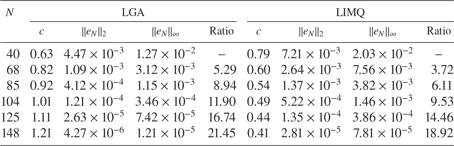
Some numerical results for Example 4.2 using the proposed method.
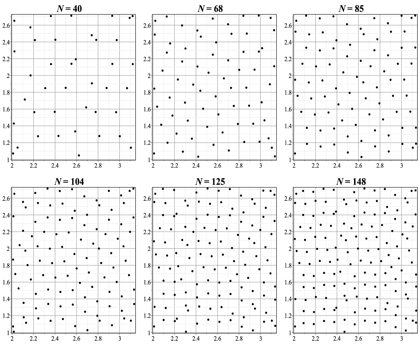
Node distribution for Example 4.2.

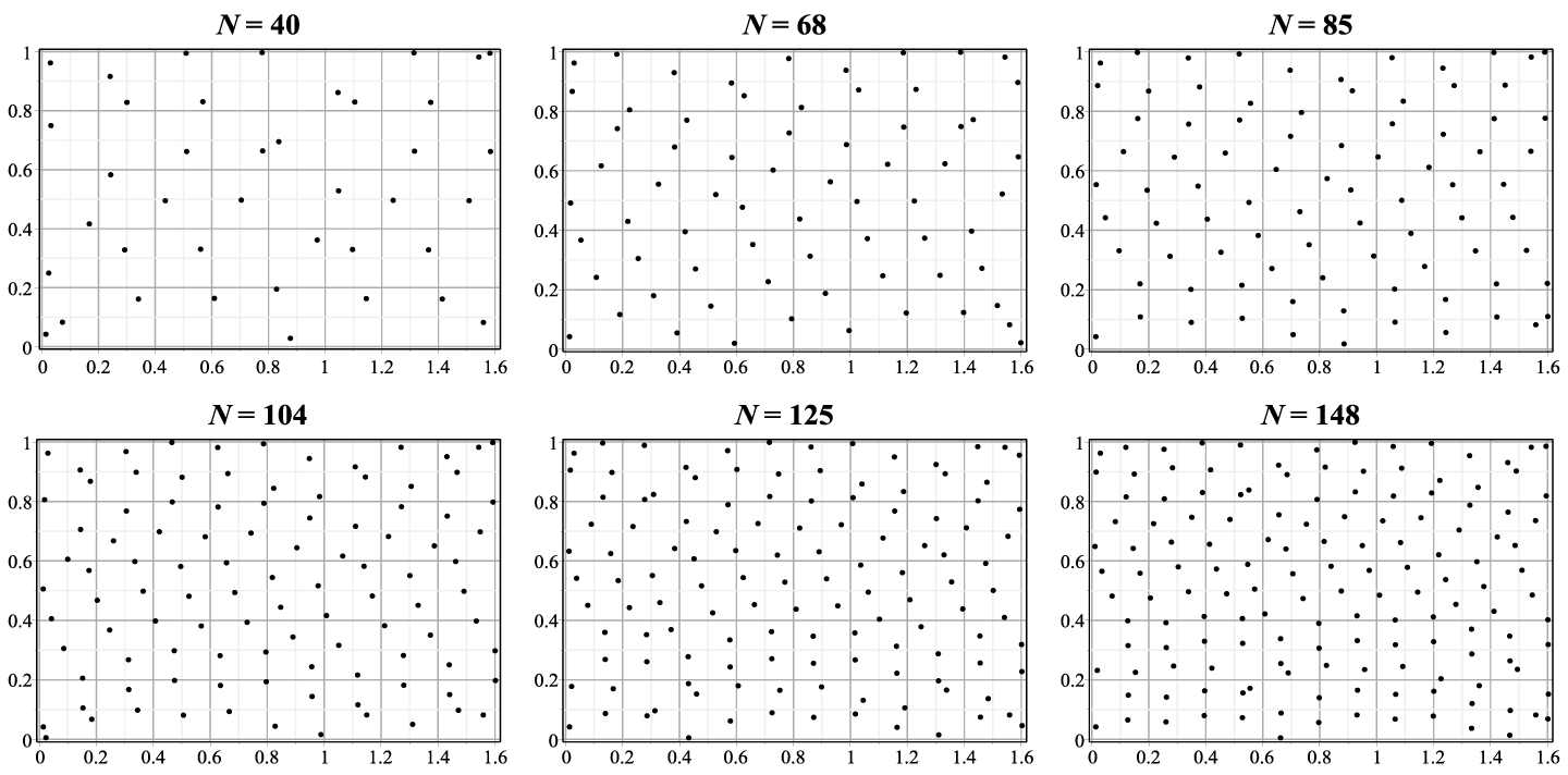
Previous numerical methods have difficulties in solving these types of integral equations, but we can easily compute the approximate solution for this problem utilizing the meshless method presented in this work based on some random nodes selected on
 $[2,\pi ] \times [1,e]$
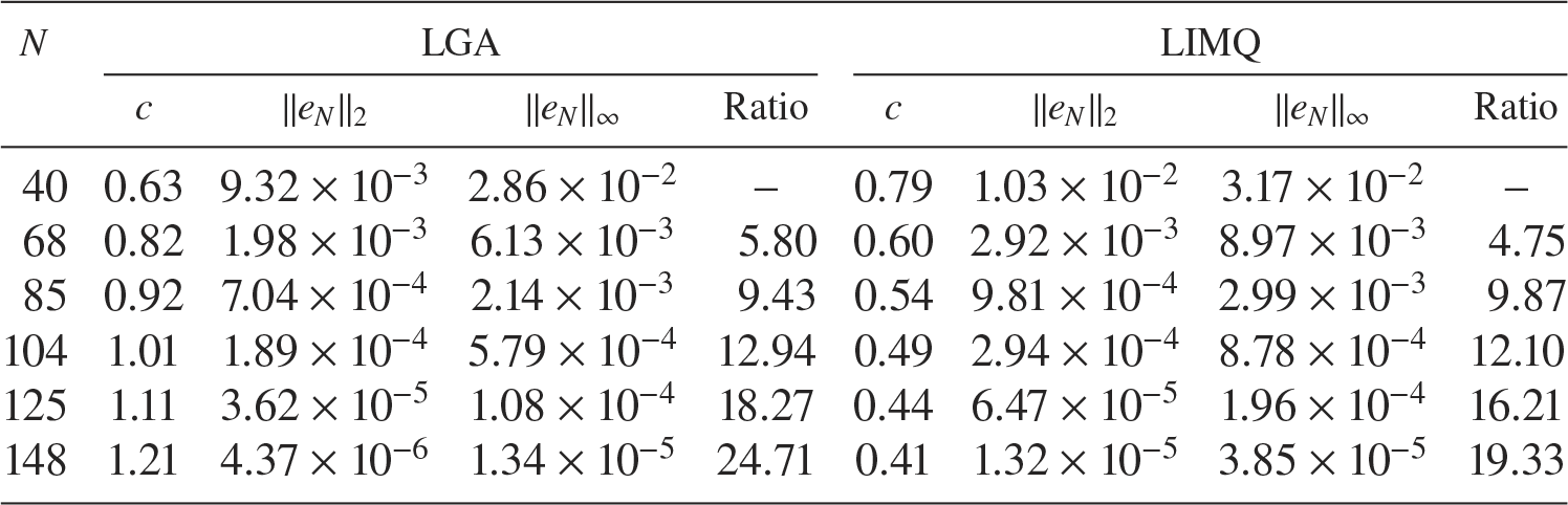
which are drawn in Figure 3. Table 2 records
 $\|e\|_{\infty }$
,
 $\|e\|_2$
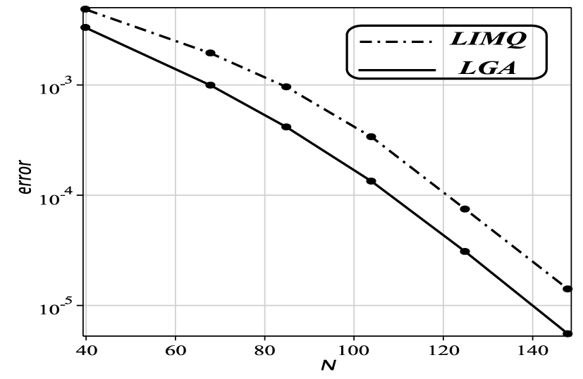
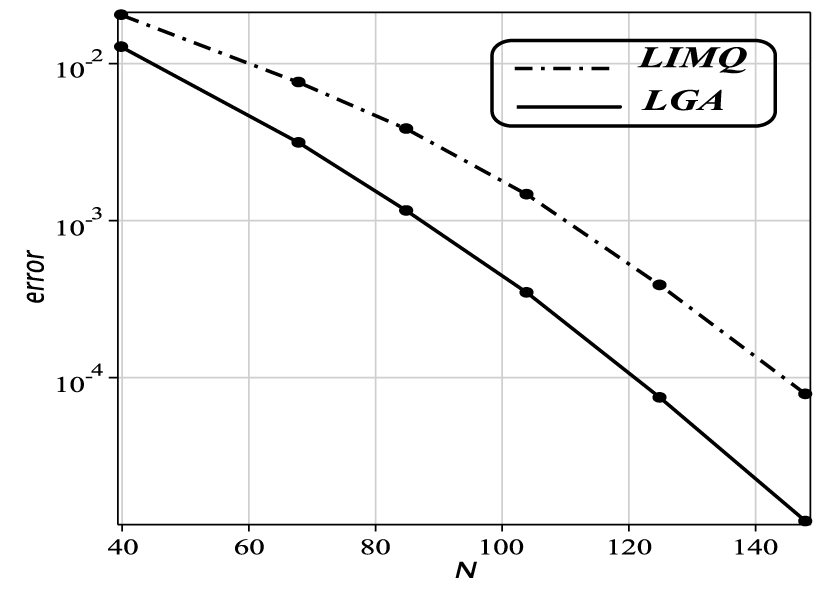
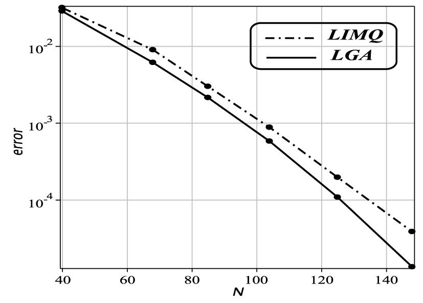
and the values of the ratio at different values of N. The errors obtained for different N are drawn on a logarithmic scale in Figure 4. The error bound (3.20) yields that for sufficiently large integration nodes the error of the LRBFs is dominated by the error of the integration rule and so increasing
 $m_N$
has no significant effect on the global error and the approximation order of the proposed method is of higher order.
Distribution of absolute error for Example 4.2.

Example 4.3 Consider the two-dimensional Darboux equation
 $$ \begin{align*} u_{xt}=2\cos^2(x+t+10)u^3(x,t)+u(x,t),\quad (x,t)\in [0,5/3] \times [2,11/3], \end{align*} $$
with conditions
 $$ \begin{align*} \begin{array}{ll} u(x,2)=\sec(x+12),&0\leq x\leq 5/3,\\ u(0,t)=\sec(t+10),&2\leq t\leq 11/3, \end{array} \end{align*} $$
and exact solution
 $u_{\mathrm {ex}}=\sec (x+t+10).$
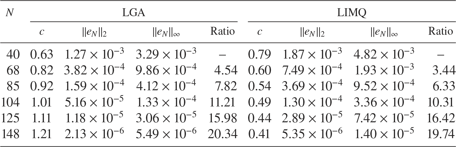
Table 3 reports
 $\|e\|_{\infty }$
,
 $\|e\|_2$
and the values of the ratio at different values of N. The errors obtained for different N are drawn on a logarithmic scale in Figure 5. We have also compared the CPU times for solving the Darboux equation (4.1) using global and local RBF for different N in Figure 6. These results show that the method presented in the current paper, in comparison with the method based on the globally supported RBFs for solving Darboux equations, requires much less computer memory and time.
Some numerical results for Example 4.3 using the proposed method.

Distribution of absolute error for Example 4.3.

CPU times for Example 4.3.

Node distribution for Example 4.4.

Distribution of absolute error for Example 4.4.

Example 4.4 Consider the two-dimensional Darboux equation
 $$ \begin{align*} u_{xt}= - \frac{1}{(x+t+\pi)^3}e^{u(x,t)},\quad (x,t)\in [0,\ln5] \times [0,1], \end{align*} $$
with conditions
 $$ \begin{align*} \begin{array}{ll} u(x,0)=\ln(x+\pi),&0\leq x\leq \ln 5,\\ u(0,t)=\ln(t+\pi),&0\leq t\leq 1, \end{array} \end{align*} $$
and exact solution
 $$ \begin{align*}u_{\mathrm{ex}}=\ln(x+t+\pi).\end{align*} $$
Table 4 reports
 $\|e\|_{\infty }$
,
 $\|e\|_2$
and the values of the ratio at different numbers of N. The distribution of nodes, selected randomly on the interval
 $[0,\ln 5] \times [0,1]$
, is depicted for some values of N in Figure 7. The errors obtained for different N are drawn on a logarithmic scale in Figure 8. It should be noted that from the error bound (3.20), the results gradually converge to the exact values as the number of nodes increases. Therefore, the numerical results confirm the theoretical error estimates.
Some numerical results for Example 4.4 using the proposed method.

5 Conclusion
In this paper, we have proposed an efficient and computationally attractive scheme based on locally supported RBFs as a basis in the Galerkin method to solve nonlinear two-dimensional Darboux equations. The integrals arising in this approach have been computed utilizing the Gauss–Legendre integration rule. This method converts the solution of the Darboux equation into the solution of a system of algebraic equations. In comparison with globally supported RBFs for solving integral equations, the proposed method is stable and uses much less computer memory. Since the scheme does not need any cell structure, it can be identified as a meshless method. We also have obtained the error bound and the convergence rate of the method. As demonstrated by the numerical results, the proposed technique is able to produce highly accurate solutions with less CPU time for various types of Darboux equations. In the following, we list some limitations of the proposed method which can be improved in future research.
-
• The proposed method can be developed for integral equations over nonrectangular domains.
-
• The investigation of optimal values for shape parameters in general is not straightforward.
-
• A suitable integration rule can be used to expand the method on singular integral equations.
-
• Theoretical analysis is only developed for the Darboux problems with solutions in real native Hilbert spaces.
-
• The error of the method is obtained based on a quasi-uniform set and not on an arbitrary set.
Acknowledgements
The authors are most grateful to the reviewers for their valuable comments and suggestions which improved the paper.