2.1 Controlling the family wise error rate

We now assume that the researcher is interested in maximizing power while controlling the Family Wise Error Rate (FWER).

The most basic way of controlling the FWER is to make Bonferroni adjustments: instead of rejecting $H_{0}$ if the $p$ value is smaller than $\unicode[STIX]{x1D6FC}$ , reject if it is smaller than $\unicode[STIX]{x1D6FC}/m$ .Footnote ¹⁰ The main issue is that the method is only valid if the researcher can keep track of all tests she performed. If for example, the researcher ran $m^{\prime }$ tests and attempt to control the FWER as if only $m$ tests had been carried out (with $m<m^{\prime }$ ), the reported FWER will underestimate the actual FWER. As a result, we rule out that the researcher can implement the Bonferroni adjustments without a PAP.

2.1.1 Procedure 1: Preanalysis plan with Bonferroni corrections

Before having access to the data, the researcher can prepare and register a PAP (Humphreys, Sanchez de la Sierra, and van der Windt Reference Humphreys, Sanchez de la Sierra and van der Windt2013; Olken Reference Olken2015; Dunning Reference Dunning2016). Such a plan lists the hypotheses to be tested and describes how they will be tested, including which variables to include, how they will be included, and how researchers intend to deal with the multiple comparison problems.

The main drawback of PAPs is that they do not allow researchers to learn from the data, and this can slow down the pace of new discoveries. PAPs can only cover hypotheses that the researcher could think of before carrying out their experiment. There often are other testable hypotheses that the researcher did not think of beforehand. A number of social scientists have recently argued that some of their most important findings were the direct result of time spent with the data (Laitin Reference Laitin2013; Gelman Reference Gelman2014). For example, Simonsohn (cited by Laitin (Reference Laitin2013)) argues that: “I also think of science as a process of discovery ... Every paper I have [written] has some really interesting robustness, extensions, follow-ups that I would have never thought about at the beginning.” Similarly, Gelman (Reference Gelman2014) states that “Many of my most important applied results were interactions that my colleagues and I noticed only after spending a lot of time with our data.”

To capture those constraints, we assume that the researcher picks a subset $m^{\prime }$ of the $m$ variables that might be affected by the treatment. This includes $m_{0}^{\prime }$ true null hypotheses and ( $m^{\prime }-m_{0}^{\prime }$ ) nontrue null hypotheses. Those $m^{\prime }$ variables are included in the PAP. A crucial parameter in this context is $\unicode[STIX]{x1D713}$ : the likelihood that variables for which the null hypotheses is nontrue are included in the PAP. To put it differently, $\unicode[STIX]{x1D713}$ captures the degree of uncertainty surrounding the effects of $T$ ; or the degree of prior information available.

Rejecting a given hypothesis in this setup requires that the hypothesis is included in the subset $m^{\prime }$ and that it is rejected on the full sample. Let $\unicode[STIX]{x1D6FC}$ be the significance level used to test $H_{0}^{k}$ and let $\unicode[STIX]{x1D6FF}_{k}$ be the standardized effect size for the $m-m_{0}$ nontrue null hypotheses. Under our assumptions, power is given by:

(2) $$\begin{eqnarray}1-\unicode[STIX]{x1D6FD}_{k}^{PAP/Bonf}=\unicode[STIX]{x1D713}\ast \unicode[STIX]{x1D6F7}\left(\unicode[STIX]{x1D6FF}_{k}\sqrt{\frac{N}{4}}-Z_{1-(\unicode[STIX]{x1D6FC}/2m^{\prime })}\right)\end{eqnarray}$$

where $\unicode[STIX]{x1D6F7}$ is the cumulative distribution function for the standard normal distribution. More details on the calculations are provided in the technical appendix. As the researcher implements $m^{\prime }$ tests at level $\unicode[STIX]{x1D6FC}/m^{\prime }$ she controls the FWER at level $\unicode[STIX]{x1D6FC}$ .

2.1.2 Procedure 2: Sample split with Bonferroni adjustments

We now outline the main characteristics of the split sample approach. More practical guidelines on how to implement the procedures are provided in Section 4.

• ∙ Step 1: Guided by theory and existing evidence, researcher $A$ puts together a sample $S$ including a number of variables that broadly captures the general set of hypotheses that she wants to test. The researcher also includes variables used to test for potential heterogeneous effects. This step is likely to include extensive data cleaning.

• ∙ Step 2: A third party $B$ randomly generates two nonoverlapping subsets. If the researcher is interested in studying particular subgroups the sample should be stratified accordingly. The first subsample (training sample) is sent back to $A$ . The third party keeps the second one (testing sample). All relevant IDs are scrambled during the process so that $A$ is unable to “reverse engineer” the randomization.

• ∙ Step 3: $A$ runs regressions, presents the results at seminars and conferences, and refines the methodology based on feedback received.

• ∙ Step 4: The paper is submitted to a journal, referees make their comments and $A$ amends her analysis in response, possibly several times.

  The discovery process described by steps 3 and 4 identifies a final subset $J$ of the $m$ outcome variables. We call this the final methodology for analysis. One option is to select outcome variables for which we can reject the null of no effect at the $\unicode[STIX]{x1D6FC}$ level in the training set, conditional on a choice of estimator, control variables, and standard error correction.

• ∙ Step 5: Once the editor is satisfied that the estimation strategy is reliable, she accepts the paper conditional on the agreed upon final methodology for analysis. $A$ then secures the testing sample from $B$ and applies the agreed upon methodology to it. The published version of the paper includes the results obtained from the testing sample with adequate $p$ -values adjustments to deal with multiple testing. In essence, this final step allows researchers to perform a direct replication of their findings. We nonetheless recommend that the results from the training sample be made available as an appendix to the paper, e.g., for an interested (Bayesian) reader or for possible inclusion in a meta-analysis.

Throughout we assume that the researcher starts with $m$ possible null hypotheses. Of these, a subset $J$ are found to be significant at the $\unicode[STIX]{x1D6FC}$ level in the training set and interesting. This subset determines the list of tests estimated on the testing set. To illustrate, let $m=20$ and imagine that, in the training sample, treatment is significant at the $\unicode[STIX]{x1D6FC}=5\%$ level for seven of these $20$ outcome variables. Then we only regress treatment on these seven outcome variables in the testing sample.

For an hypothesis to be rejected, it is necessary that it be rejected first on the training sample, and then again on the testing sample. We assume that researchers allocate a share $s$ of their data to the training sample and that they use significance level $\unicode[STIX]{x1D6FC}_{tr}$ on the training sample and $\unicode[STIX]{x1D6FC}$ on the testing sample. As the training and testing samples are independent, power becomes:

(3) $$\begin{eqnarray}1-\unicode[STIX]{x1D6FD}_{k}^{Split/Bonf}=\unicode[STIX]{x1D6F7}\left(\unicode[STIX]{x1D6FF}_{k}\sqrt{\frac{sN}{4}}-Z_{1-\unicode[STIX]{x1D6FC}_{tr}/2}\right)\unicode[STIX]{x1D6F7}\left(\unicode[STIX]{x1D6FF}_{k}\sqrt{\frac{(1-s)N}{4}}-Z_{1-\unicode[STIX]{x1D6FC}/2B}\right)\end{eqnarray}$$

where $B$ is the number of tests carried out on the testing sample. $B$ corresponds to the number of rejections in the training sample, aggregating across both true positives and false positives. It is the sum of two binomial-distributed random variables. The fist has distribution $B(m_{0},\unicode[STIX]{x1D6FC}_{tr})$ ; the second has distribution $B\left(m-m_{0},\unicode[STIX]{x1D6F7}\left(\unicode[STIX]{x1D6FF}_{k}\sqrt{\frac{sN}{4}}-Z_{1-\unicode[STIX]{x1D6FC}_{tr}/2}\right)\right)$ . Their sum is distributed according to:

(4) $$\begin{eqnarray}B\sim B(m_{0},\unicode[STIX]{x1D6FC}_{tr})+B\left(m-m_{0},\unicode[STIX]{x1D6F7}\left(\unicode[STIX]{x1D6FF}_{k}\sqrt{\frac{sN}{4}}-Z_{1-\unicode[STIX]{x1D6FC}_{tr}/2}\right)\right).\end{eqnarray}$$

As above the researcher implements $B$ tests at level $\unicode[STIX]{x1D6FC}/B$ and so she controls the FWER at level  $\unicode[STIX]{x1D6FC}$ .

Setting a critical value for the training sample ( $\unicode[STIX]{x1D6FC}_{tr}$ ) involves trading off a larger number of rejections on the training sample for a lower probability of rejection on the testing sample due to multiple testing adjustment. The above formulas show that the optimal value of ( $\unicode[STIX]{x1D6FC}_{tr}$ ) is a function of the number of hypotheses, the number of true null hypotheses, the sample size, and the distribution of effect sizes across all hypotheses. Should a researcher be willing to assume the number of true null hypotheses and the distribution of effect sizes across all hypotheses in their data, the formulas can be used to numerically derive the optimal critical value for a particular sample size and number of tested hypotheses.

2.2 Controlling the false discovery rate

We now assume that researchers are interested in maximizing power while controlling the False Discovery Rate (FDR). The concept, introduced Benjamini and Hochberg (Reference Benjamini and Hochberg1995), captures the idea that, in a number of relevant cases, it is acceptable to reject true null hypotheses as long as such rejections constitute a small share of total rejections. The intuition is that the decision maker would reach the same conclusion regardless of whether or not those true null hypotheses are rejected.

Benjamini and Hochberg (Reference Benjamini and Hochberg1995) proposed a method to control the FDR. The BH method proceeds as follows:

1. (1) Carry out the m tests and get the associated $p$ values $p_{1},\ldots ,p_{m}$

2. (2) Rank the $p$ values from smallest to largest $p_{(1)},\ldots ,p_{(m)}$

3. (3) Get $k=Max\{i|p_{(i)}\leqslant \frac{i}{m}q\}$ . $q$ is the level at which the researcher would like to control the FDR.

4. (4) Reject all $H_{(i)}$ for $i\leqslant k$

Benjamini and Yekutieli (Reference Benjamini and Yekutieli2001) show that the method is conservative as it controls the FDR at level $\frac{m_{0}}{m}q$ . The proof relies on the fact that while for true null hypotheses the $p$ values are uniformly distributed over $[0,1]$ , they tend to be bunched toward 0 for nontrue null hypotheses. As a result, when observing two $p$ values the hypothesis associated with the smallest one is more likely to be nontrue. Simulations presented in Benjamini and Hochberg (Reference Benjamini and Hochberg1995) indicate that power is significantly larger than for methods that control the FWER. Benjamini, Krieger, and Yekutieli (Reference Benjamini, Krieger and Yekutieli2006) extend the method to a two-stage procedure where the first stage is used to get an estimate of $m_{0}$ . The sharpened $q$ values are obtained as follows:

1. (1) Apply the BH procedure at level $q^{\prime }=q/(1+q)$ . Let $c$ be the number of hypotheses rejected. If $c=0$ , stop; otherwise, continue to step 2.

2. (2) Let $\hat{m}_{0}=M-c$

3. (3) Apply the BH procedure at level $q^{\ast }=q^{\prime }m/\hat{m}_{0}$

In the simulations we compare a PAP with our sample-split approach with sharpened $q$ values. The trade-offs are similar as before but both methods are expected to deliver higher power than when researchers wanted to control FWER.

3.1 Main results

We illustrate the method for the canonical setup described above. We compute power and FWER under the full sample approach with a PAP and the split sample approach.Footnote ¹¹ In both cases, we present results with Bonferroni adjustments. We show the sensitivity of power and FWER to variation in the following parameters: prior information ( $\unicode[STIX]{x1D713}$ ); the sample size ( $N$ ); the standardized effect size ( $\unicode[STIX]{x1D6FF}$ ); the number of tested hypotheses ( $m$ ); the number of tested null hypotheses that are true ( $m_{0}$ ); and the share of the total sample that is allocated to the training set ( $s$ ).

We present results from applying the above formulas and simulation methods to various parameter values. To capture the idea that there are many more true null hypotheses than false ones (Ioannidis Reference Ioannidis2005), we organize the simulations around the assumption that, out of $100$ possible null hypotheses, only one is nontrue, i.e., should be rejected. Hence, unless stated otherwise, the results presented below are based on $m=100$ and $m_{0}=99$ .

Given these parameter values, the majority of the results found significant are spurious. For instance, if $\unicode[STIX]{x1D6FC}=5\%$ , there will on average be five false rejections and, provided that power is high enough, one true rejection in the training sample. For now we use a 50–50 split between the training and testing samples, i.e., we set $s=0.5$ .

We organize our simulations around two stylized testing scenarios: (1) testing 10 null hypotheses on the full sample with Bonferroni corrections (with $\unicode[STIX]{x1D713}=0.25,0.50,0.50$ or $1$ ); (2) testing all 100 null hypotheses on the training sample, and only testing (with Bonferroni corrections) on the testing sample those null hypotheses that were significant in the training sample. We assume that we only test 10 hypotheses on the full sample to capture the idea the researcher writes a PAP.

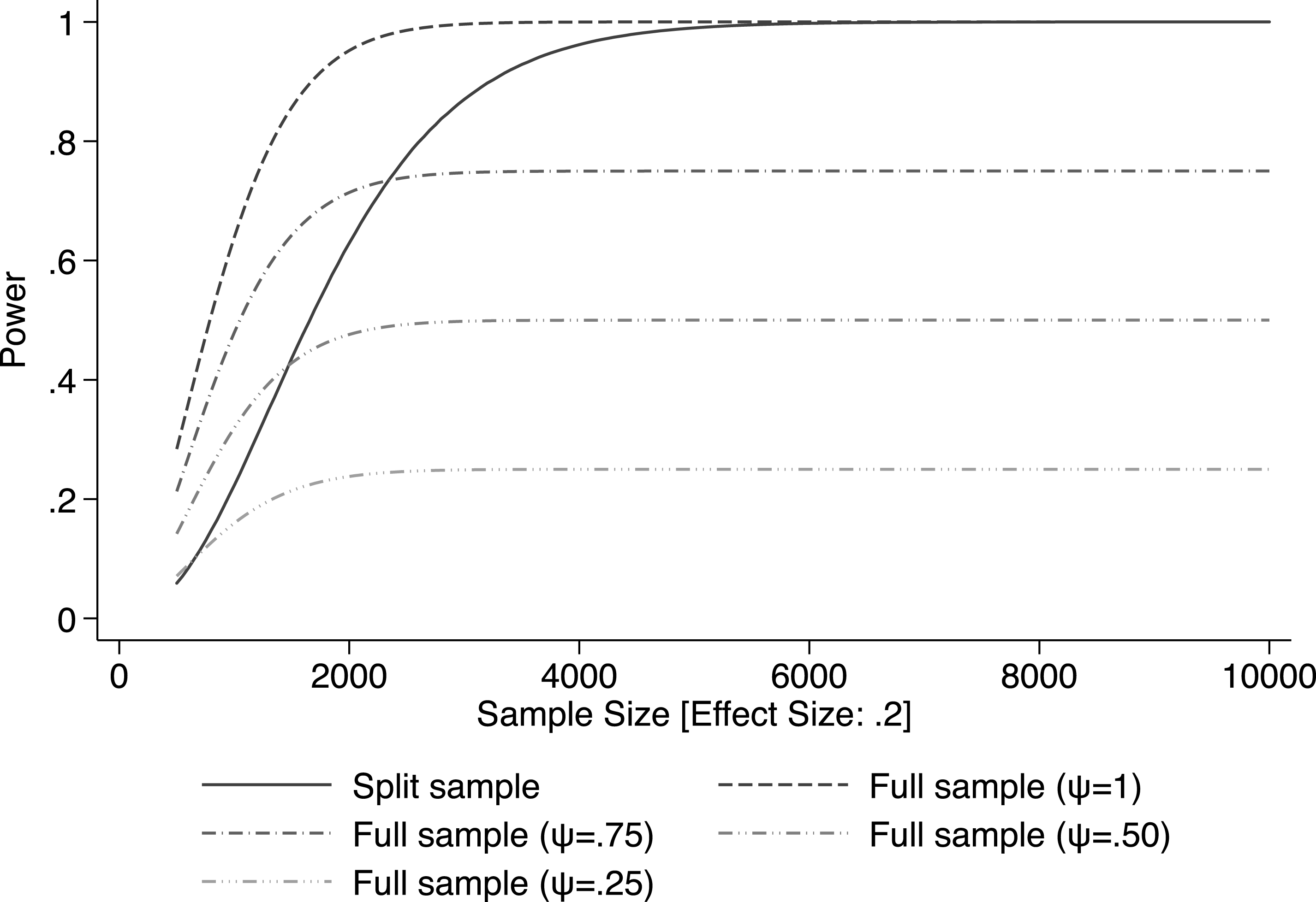
Role of  $N$ and  $\unicode[STIX]{x1D713}$ . We start by investigating the effect of sample size on the power to detect a true effect of size 0.2. In other words, we compute the likelihood of rejecting the null hypothesis when this hypothesis is false and the true effect is 0.2. Figure 1 plots power under the scenarios for sample sizes varying between 500 to 10,000. Power under the split sample approach is well above 0.8 for the kind of sample sizes of 3,000 or more that are commonly encountered in empirical work. Importantly, the PAP strictly dominates the split sample approach only when the amount of prior information is very high. In situations where $\unicode[STIX]{x1D713}$ is lower, the split sample approach actually delivers more power than a PAP. If $\unicode[STIX]{x1D713}=.75$ the split sample dominates the PAP as soon as $N$ is larger than 2,300. The split sample delivers more power than a PAP as soon as $N$ is larger than 700 (respectively 1,500) when $\unicode[STIX]{x1D713}$ is equal to 0.25 (respectively 0.50).

Figure 1.

Comparing power: full sample vs. split sample [effect size $=$ 0.2].

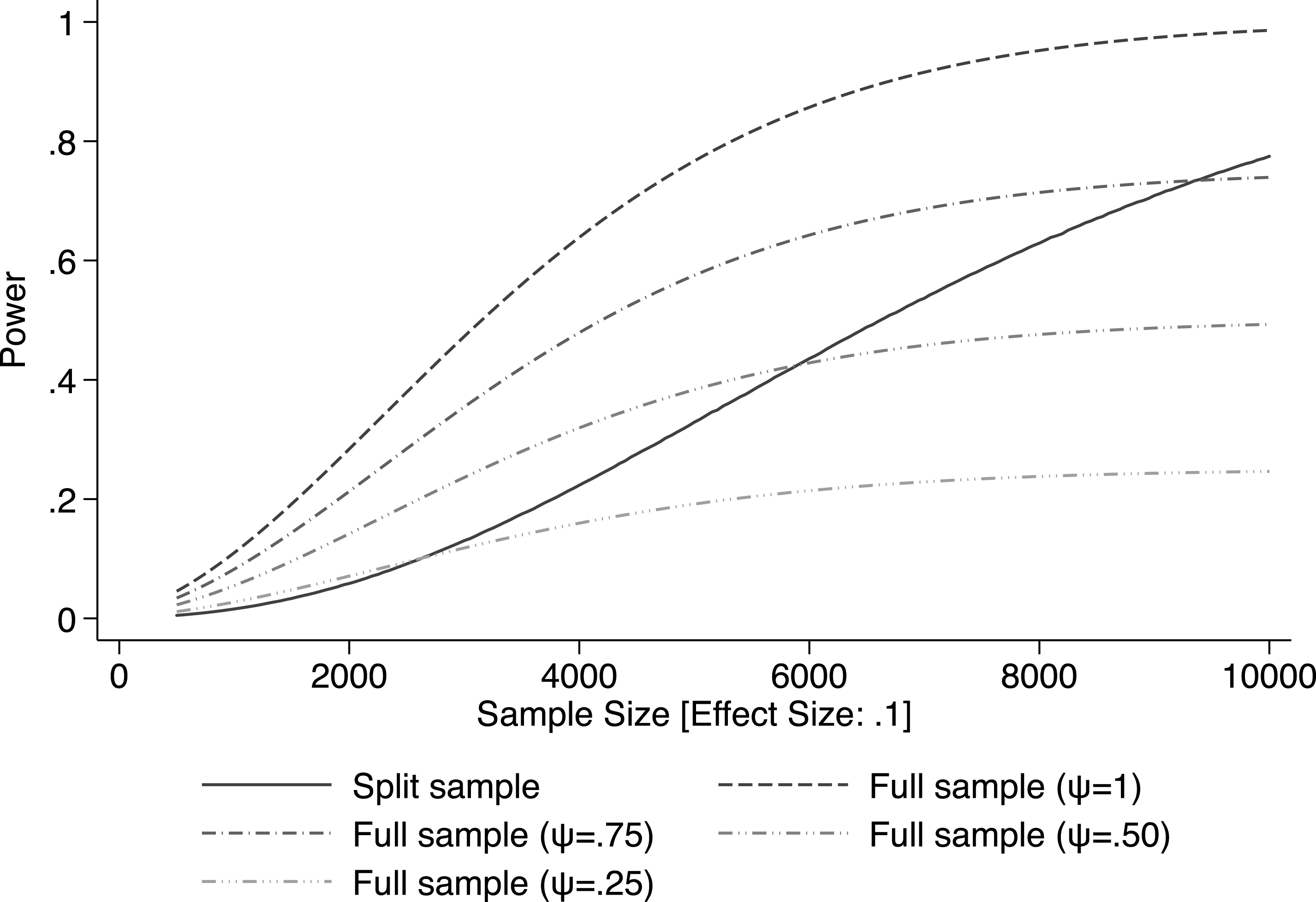
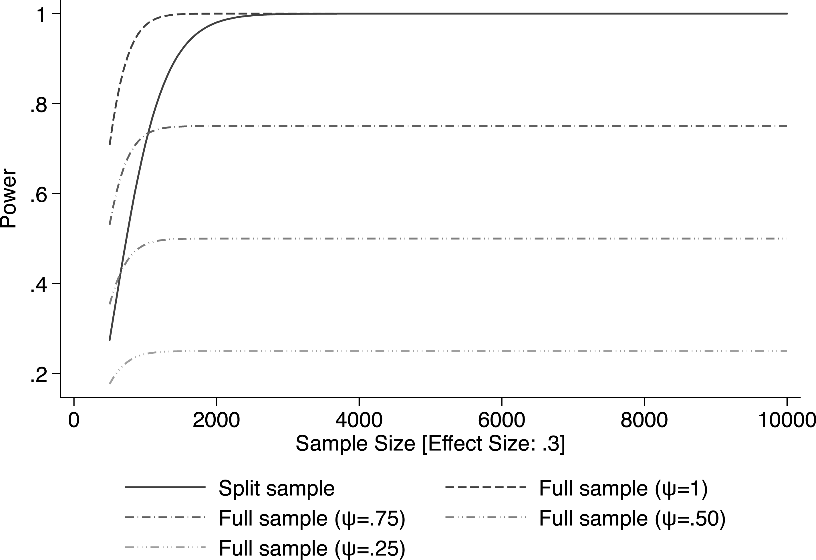
Figures 2 and 3 plot similar results for different effect sizes of 0.1 and 0.3. Larger, but still relatively common, sample sizes are required to have power above 0.8 with smaller expected effect sizes (Figure 2). For example, with a small expected effect size of 0.1, raising power above 0.8 under the split sample approach requires sample sizes of 10,000 or more. As above, the split sample dominates a PAP for low values of $\unicode[STIX]{x1D713}$ and medium sample sizes.

Figure 2.

Comparing power: full sample vs. split sample [effect size $=$ 0.1].

Figure 3.

Comparing power: full sample vs. split sample [effect size $=$ 0.3].

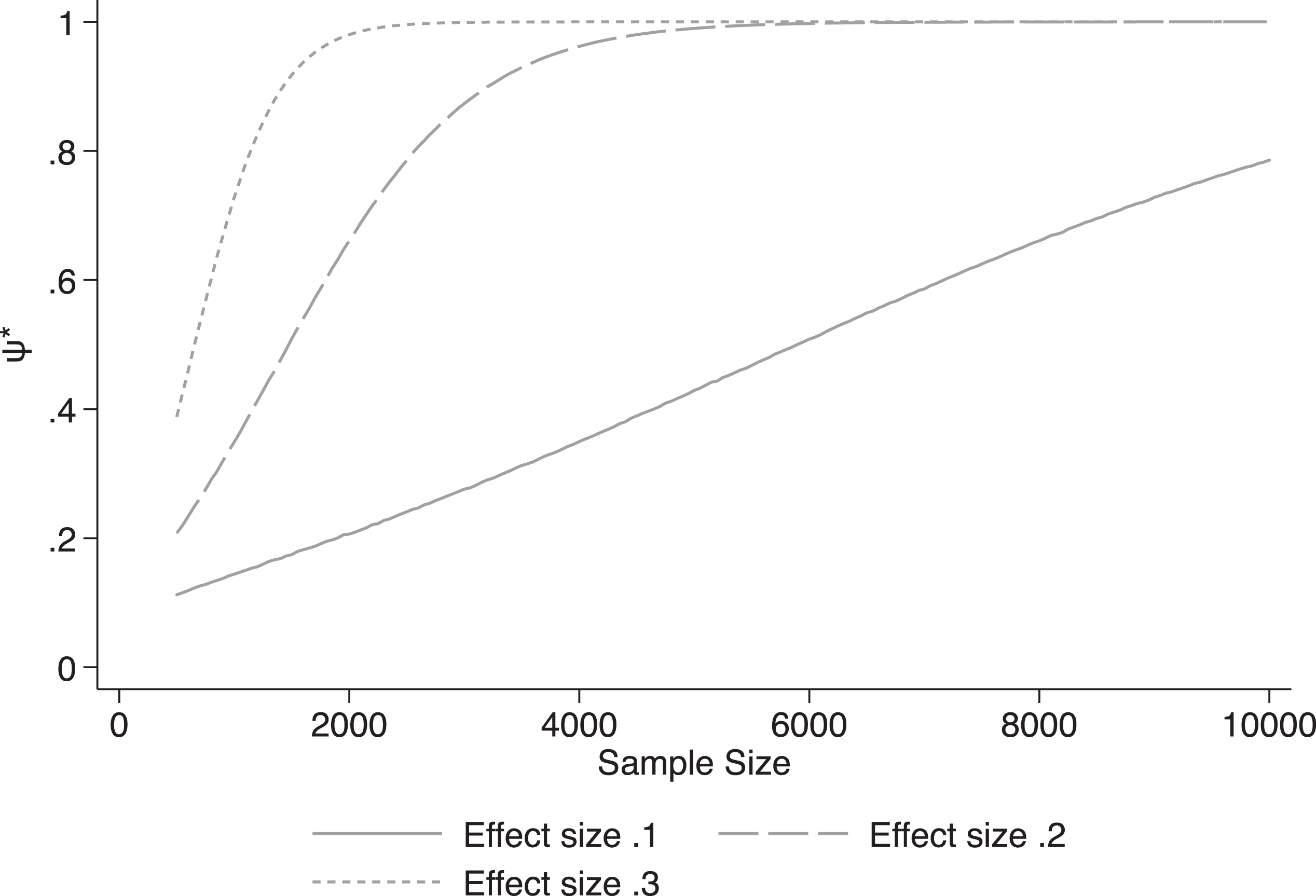
Researchers’ ability to learn. As argued above, the split sample approach has an important benefit: it allows the researcher to test a large number of hypotheses with little loss in power. Using formulas for power discussed in Section 2.1, we can compute the value $\unicode[STIX]{x1D713}^{\ast }$ at which the two methods yield similar power. In Figure 4, we plot the value of $\unicode[STIX]{x1D713}^{\ast }$ for various effect sizes (0.1, 0.2 and 0.3). For all values of $\unicode[STIX]{x1D713}$ below the curve, the split sample approach delivers more power. In a large number of cases, $\unicode[STIX]{x1D713}$ needs to be close to one for the full sample approach with a PAP to be superior (or equivalent) to the split sample approach. For example, for effect sizes of 0.3 as soon as sample size is above 2,000, $\unicode[STIX]{x1D713}$ needs to be one for the two approaches to yield similar results. Even with an effect size of 0.1 and a sample size of 7,000, $\unicode[STIX]{x1D713}$ needs to be above 0.6 for the full sample approach with a PAP to dominate. This set of results thus confirms that the split sample approach increases researchers’ ability to learn from the data.

Figure 4.

Value of $\unicode[STIX]{x1D713}$ at which the full sample approach with a PAP and the split sample approach yields the same power. Note:  $\unicode[STIX]{x1D713}$ is the likelihood that the nontrue hypothesis is in the set of tests included in the PAP.

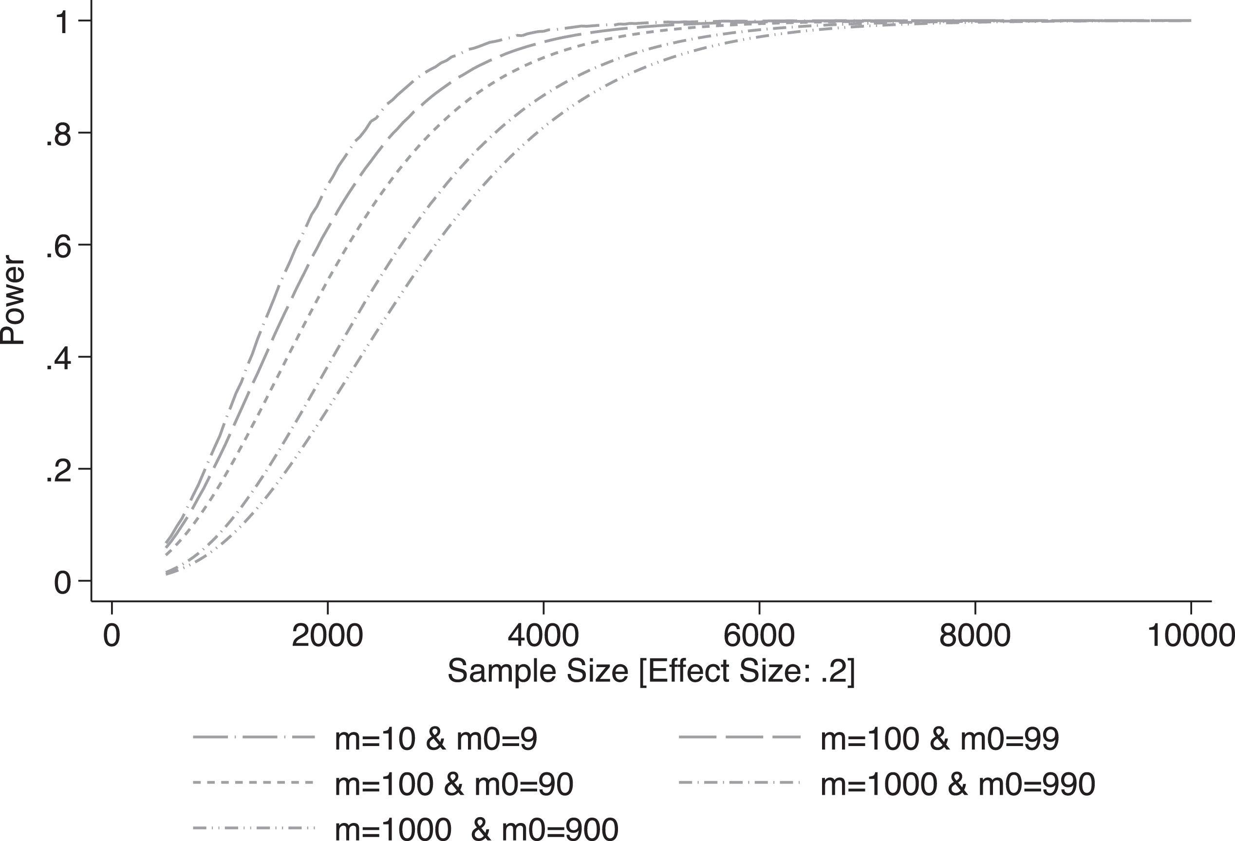
Role of the number of variables ( $m$ ). So far we have set $m=100$ and $m_{0}=99$ . Next, we simulate what happens to power when we vary the total number of hypotheses that are being tested ( $m$ ) and the number of nontrue hypotheses ( $m_{0}$ ). The effect size that we are trying to detect is 0.2, as in Figure 1. Figure 5 shows our simulation results for scenario (2)—the split sample approach with Bonferroni correction applied to the testing sample results. Results show that power is a decreasing function of $m$ and $m_{0}$ . This is because the Bonferroni correction becomes more stringent as $m$ or $m_{0}$ increase.

Figure 5.

Power under the sample-split approach with Bonferroni corrections: number of variables.

Role of the share of the total sample that is allocated to the training set ( $s$ ). We also investigate whether it is optimal to split the sample 50–50 between training and testing sets. We continue to focus on scenario (2)—sample split with Bonferroni corrections—and we simulate power under alternative sample splitting rules, i.e., $30/70$ and $70/30$ . The results, displayed in Figure A.1, indicate that, across all considered sample sizes, a $50/50$ split delivers the best power.

Role of the decision rule on the training sample. Next, we investigate whether power in the split sample approach with Bonferroni correction depends on the threshold level of significance used to select hypotheses in the training sample. So far we have assumed that this threshold is the same in the training and testing samples, i.e., $\unicode[STIX]{x1D6FC}=0.05$ . We now compare this situation to using a threshold of $0.1$ when selecting hypotheses on the training sample. Three effect sizes are considered: $0.1,0.2$ and $0.3$ . We find that, for all three effect sizes, power appears to be marginally larger with a 0.05 threshold than a 0.1 threshold (Figure A.2). This is because applying a less restrictive threshold to the training sample increases the number of true null hypotheses that are rejected, and thus the number of hypotheses that are tested on the testing sample. A larger number of hypotheses means that a stronger Bonferroni correction is required on the testing sample, and this results in a loss of power. It is important to note that this finding is somewhat driven by our stated assumptions that $m=100$ and $m_{0}=99$ . These assumptions are intended to capture the fact that there are many more true hypotheses than false ones Ioannidis (Reference Ioannidis2005). However, in the extreme case $m=m_{0}=1$ , a higher threshold in the training sample will deliver higher power.

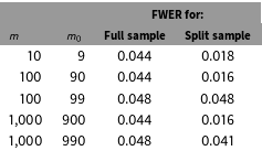
FWER. Having compared the two statistical procedures—the PAP and the split sample approach—in terms of power, we now compare in terms of their ability to minimize the risk of false rejection. In Table 1 we compare the FWER under our two scenarios. Recall that the FWER is the probability of rejecting at least one true null hypothesis. As expected given that we use Bonferroni corrections, the FWER is below 5% under both methods.

Figure 6.

Comparing power with sharpened $q$ values: full sample vs. split sample [effect size $=$  0.2].

Table 1.

Comparing the Family Wise Error Rate with the 2 methods.

Notes: authors’ calculations.

3.2 Extensions

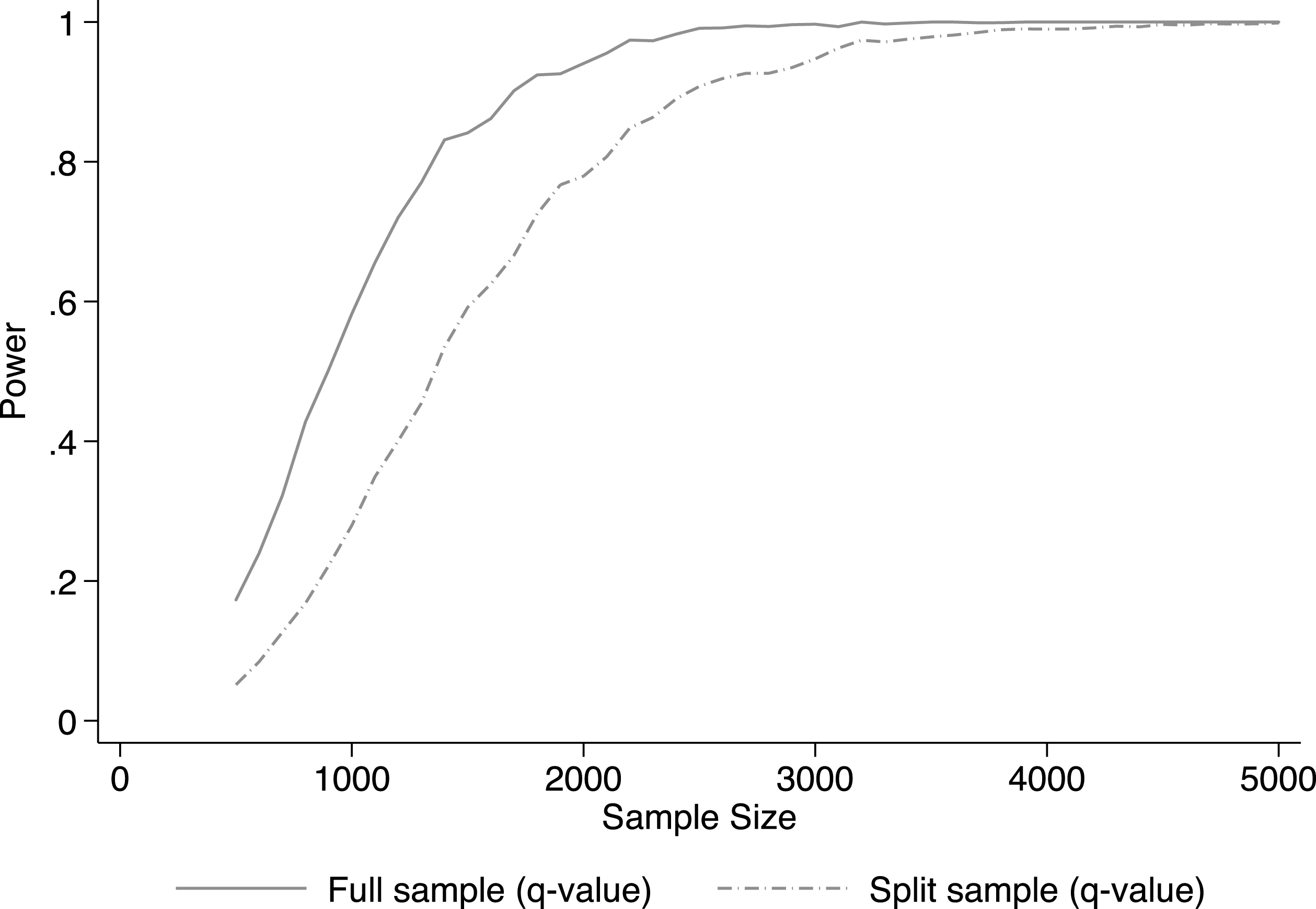
Controlling the FDR. We now compare the two procedures if the researcher is interested in controlling the FDR rather than the FWER. We run simulations computing $q$ values for $m=100$ , $m_{0}=90$ , $\unicode[STIX]{x1D6FF}=0.2$ and sample sizes varying from 500 to 5,000 in 100 increments using the method described in Section 2.2. We assume that half of the observations are allocated to the training set. For both the full sample and the split sample approach we compute power as the share of the 1,000 iterations for which the $q$ value is below 0.05. Results are available in Figure 6. As expected under both the full sample and the split sample approaches, power is higher when using sharpened $q$ values than when using Bonferroni corrections. In addition, power under the split sample approach is now above 0.8 as soon as sample sizes are larger than 2,000 observations. Importantly those results assume that $\unicode[STIX]{x1D713}=1$ . Given the narrow gap between power with a PAP and power with the split sample approach, the split sample approach will dominate the PAP if $\unicode[STIX]{x1D713}$ is below 0.5 for sample sizes of about 1,000 and if $\unicode[STIX]{x1D713}$ is below 0.8 for sample sizes of about 2,000.

Clustered samples. Up to now we have assumed that researchers have access to an unclustered sample (or that intercluster correlation is sufficiently low to be ignored). In a number of settings this assumption is likely to be violated and we now report results from simulations with clustered samples. In a sample with $c$ clusters and an intracluster correlation coefficient of $\unicode[STIX]{x1D70C}$ power is given by:

(5) $$\begin{eqnarray}1-\unicode[STIX]{x1D6FD}_{k}^{\mathit{Clustered}}=\unicode[STIX]{x1D6F7}\left(\unicode[STIX]{x1D6FF}_{k}\sqrt{\frac{N}{4\ast (1+(c-1)\unicode[STIX]{x1D70C})}}-Z_{1-\unicode[STIX]{x1D6FC}/2}\right).\end{eqnarray}$$

We can easily adjust the formula to obtain power both for the full sample approach and the split sample approach with Bonferroni corrections. As before, we run 10,000 simulations. We compute power for sample sizes varying from 500 to 10,000 with 20 observations per clusters. We assume that $\unicode[STIX]{x1D70C}$ is either $0.05$ or $0.1$ . To ensure that the two samples are independent we sample full clusters rather than individuals within clusters. The sample split therefore leads to the loss of half of the clusters rather than to the loss of half of the observations per cluster. Results are available in Figure A.3. As expected power is lower than what it is with an unclustered sample. For example, with $\unicode[STIX]{x1D70C}=0.05$ power is above 0.8 with the split sample approach for samples of 5,000 observations and more. If $\unicode[STIX]{x1D70C}=.1$ , sample sizes of about 8,000 are required for power to be above 0.8.

Subgroup analysis. The approach proposed here should apply equally well to subgroup analysis—analyses of a subsample/subset of the target population. To see this, one can simply think of a treatment effect regression on a subgroup as a separate regression with its own outcome variable (i.e., the outcome in the subgroup). It is immediately apparent that the smaller the subgroup is, the less informative the data will be, and the more results can be expected to vary between training and testing sample. In other words, subgroup analysis is where power issues are most stringent, and thus where our method can prove particularly useful—provided that the subgroup samples do not become too small relative to the effect size of interest. The simulations reported here can be used a guide for deciding when subgroup analysis will not be helped by a sample-split approach.

Correlated outcomes. So far we have assumed that all outcomes are uncorrelated. In many situations it is likely that some outcomes will be correlated, e.g., because different outcome variables together capture a general concept or behavior. In those situations, researchers can aggregate the outcomes into adequately defined indices (Anderson Reference Anderson2008). The split sample approach outlined here can be applied to these indices as well, although the gain in terms of power is likely to be smaller: (i) aggregating outcome variables into indices reduces the number of tested outcomes, mechanically reducing the loss of power due to corrections for multiple hypotheses testing corrections; and (ii) if constructed indices are less likely to be left out of the core analysis, this raises our parameter $\unicode[STIX]{x1D713}$ , which also reduces the gain from the split sample approach.

If the researcher is unwilling to postulate the existence of relevant indices, it is possible to conduct the analysis on the training sample as outlined here, but then apply to the testing sample a multiple hypotheses adjustment that accounts for correlation in outcome variables. The split sample approach applies to those cases as well and delivers similar benefits. The main difference is that, when outcomes are correlated, test results on the training sample are likely to be correlated as well, leading to groups of outcome variables being either dropped together, or kept in the training sample together—at which point a multiple hypotheses adjustment can be applied to account for the correlation in outcomes. For instance, Sankoh, Huque and Dubey (Reference Sankoh, Huque and Dubey1997) propose a method to control the FWER without being too conservative, while Benjamini and Yekutieli (Reference Benjamini and Yekutieli2001) offer a method that controls the FRD even when the tests have positive regression dependency.

Controlling referee degrees of freedom. In political science, referees and editors take a very active role in defining the paper’s methodology. They often suggest alternative estimation strategies, alternative outcome variables, and alternative subgroup analyses. In particular they are often interested in seeing evidence of mechanisms (e.g., does the variable of interest affect a related concept?). By design, those additional analyses cannot be incorporated in a PAP and so they are subject to the potential criticism of data mining, due to what Pepinsky (Reference Pepinsky2013) refers to as referee degree of freedom.

In the split sample approach, once researchers have been invited to revise and resubmit a paper, they will attempt to find a variable $Y$ that can be considered to proxy for the related concept introduced by the referees and for which they can reject the null. The issue is whether the additional hypothesis that the referee wants the researchers to explore is true (in the sense that it should not be rejected). Let us call $\unicode[STIX]{x1D719}$ that likelihood and $\unicode[STIX]{x1D6FE}$ the likelihood that the researchers find a $Y$ for which they can reject the null. Under the full sample approach, the probability that an error is made is then $\unicode[STIX]{x1D719}\ast \unicode[STIX]{x1D6FE}$ . Under the split sample approach, the probability that an error is made is $0.05\ast \unicode[STIX]{x1D6FE}$ . So as long as $\unicode[STIX]{x1D719}$ is larger than $0.05$ , the split sample approach yields fewer type I errors than a PAP once the editorial process has been taken into account.

4.1 Credible implementation

To ensure maximum credibility, we argue that the third party needs to be involved early on in the process. In particular, we recommend that a professional association—such as APSA—sets up a website where the data collection team can upload the data before the research team gets access to it. The researcher would then get access to a version of the dataset without the treatment dummy for a round of data cleaning. Once the data are cleaned, the random sample split is carried out and the research team is able to download the training sample.

The method is most useful for situations where researchers can credibly commit not to have seen the data before sending to a third party. This is consistent with the challenges faced by researchers writing PAPs. We expect this to be possible in a broad and diverse set of research areas.

First, there are cases in which researchers are involved in setting up data collection but rely on an intermediary to collect the data. In such a situation, researchers would ask the data collection intermediary to deposit it with the above mentioned website. This potentially applies to a large number of field experiments implemented in developing countries as well as to research projects involving data collected online (e.g., experiments carried out through MTurks).

Second, the method can also be applied by researchers using either proprietary data or nonpublicly available administrative data. The solution here is to arrange for the owner of the data to only send a random sample of it. Researchers would only have access to the remainder of the data in Step 5 discussed in Section 2.1.2.

Third, the method is also applicable in some situations where new survey data is collected, e.g., data collected in relation to the Election Research Preacceptance Competition that the Centre for Open Science organized with the 2016 American National Election Studies (ANES) data.Footnote ¹²

There nonetheless remain a number of research situations for which our method is not, at this point, implementable in a fully credible manner. For example, the approach is not currently applicable to research using publicly available data such as the Current Population Survey (CPS) collected by the US Census Bureau, The Demographic and Health Surveys (DHS) or data from the Living Standards Measurement Study (LSMS) available through the World Bank. If the split sample approach were to be become standard, however, access to new rounds of data could be organized to facilitate split sampling, as for proprietary data. The approach is also not readily suitable for researchers running their own lab experiments. Yet experimental laboratories could easily embargo the data collected in their facilities to facilitate subsequent split sample analysis. One area in which split sample analysis is not, by construction, applicable is the reanalysis of data that have been released after publication. Data reanalysis, however, typically serves a objective different from split sampling, namely, that of verifying the reliability and robustness of the published results.

4.2 Cost implications

Researchers might be concerned about the cost implications of the method. However, as the analysis in the paper makes clear, once we take into account the risk that important hypotheses are left untested. In a number of cases, power will actually be higher than under a PAP. In addition, as discussed above, the method can be combined with a PAP. For example, if the researcher has strong prior that the treatment has an effect on a subset of the variables she could submit a code to estimate those equations on the full sample—with the appropriate $p$ -value adjustments. If those results are important to guide future research the team could get access to those results when they receive the training sample.

4.3 Implications for the publication process

First, some might worry that the publication process will be bit longer as researchers have to implement the final methodology on the testing sample once the paper has been accepted for publication. We do not think that those delays will be significant however. Indeed, all the code would have been written and so running it on the testing sample should be relatively fast. In addition, allowing referees and editors to have a significant input in the finalization of the methodology might reduce the number of robustness checks that are carried out as the results will be less likely to be type I errors. This could actually speed up the publication process.

Relatedly, researchers might be worried that others will try to scoop them. As long as the potential delays discussed above are kept in check we do not think that the risk of scooping are greater than when researchers prepare a PAP. Indeed, results and draft papers will be available and presented at the same time as they would be if the researchers were to prepare a PAP.

Second, as indicated above, we expect that researchers, editors and referees will play an active role in selecting hypotheses to test on the testing sample. Some of the rejected hypotheses on the training sample might neither be interesting or relevant and thus will not be tested on the testing sample. Conversely, some important hypotheses might fail to be rejected in the training sample but might still be tested on the testing sample.

Third, editors should be less reluctant to accept a paper based on results from the training set than from a PAP design. Indeed, the split sample approach provides more information about the findings and, in the case of a RCT, about the quality of implementation. The strength of the main results and associated robustness checks on the training sample provide some information as to whether they will hold on the testing sample. In addition, one can make a case that, for well thought through hypotheses, precisely estimated zeroes should be published (as opposed to underpowered studies) and results from the training set provide useful information on the study’s statistical power.

Fourth, even in cases where the editor requires to see the results on the testing sample before accepting the paper, the authors can register a PAP containing all relevant details before running the regressions on the testing sample. If the editor declines to publish the paper after seeing the results, this would allow authors to have a record of a preregistered design when they submit the paper to another journal. That PAP would likely be superior to the one that researchers would have prepared on their own.