


1. Introduction
Consumption taxes constitute a critical fiscal policy tool for many countries, accounting for up to 50% of total tax revenue in some cases (OECD, 2020).Footnote 1 In the United States, consumption taxes are the third-largest source of total tax revenue.Footnote 2 However, compared to other OECD countries, the U.S. has the lowest share of consumption taxes in total revenue.Footnote 3 The statutory consumption tax rates on goods and services vary significantly worldwide, ranging from an average of 4.32% in the United States (2020) to as high as 27% in Hungary (2020) (OECD, 2022). This disparity raises important questions about the potential economic effects of increasing the U.S. consumption tax rate. This paper therefore investigates those effects and explores the feasibility of shifting to a progressive consumption tax system.
We conduct a series of consumption tax experiments in the context of two comparable overlapping generations (OLG) models with heterogeneous agents and uninsurable productivity risk.Footnote 4 Two models differ in their treatment of human capital: one assumes an exogenous age-productivity profile, while the other incorporates a “learning-by-doing” mechanism to model endogenous human capital accumulation (Peterman, Reference Peterman2016).Footnote 5 In both frameworks, households make consumption-savings and labor supply decisions. However, in the learning-by-doing model, accumulated work experience directly enhances future earnings capacity. To accurately assess tax policy effects, the models endogenously generate empirically plausible levels of income and wealth inequality. Following Kindermann and Krueger (Reference Kindermann and Krueger2022), we introduce high-productivity shocks to achieve realistic inequality outcomes. Each model, both the learning-by-doing version and the one with an exogenous age-efficiency profile, is calibrated to the US economy and successfully matches the targeted empirical moments. Footnote 6
We begin by analyzing the effects of a rising proportional consumption tax rate. Specifically, we increase the tax rate from 5% to 95% in 10-percentage-point increments. The simulations reveal an upward trend in aggregate capital stock, wages, labor supply, and output, while wealth inequality shows a downward trend as the consumption tax rate increases. These results indicate that shifting the tax burden from income to consumption enhances aggregate economic efficiency and, notably, reduces wealth inequality. However, several macroeconomic indicators, including aggregate consumption, government transfers, the capital–output ratio, the transfer–output ratio, the capital–labor ratio, and social welfare, exhibit hump-shaped relationships with the tax rate, suggesting diminishing welfare beyond moderate levels of taxation. Although the results of the two models exhibit similar trends, the human capital model is quantitatively more sensitive to changes in the consumption tax rate, especially at higher rates, because endogenous human capital amplifies the responses of labor productivity and capital accumulation to the tax reform. In both frameworks, social welfare is maximized when the consumption tax rate remains below 55%.
Next, we introduce an exemption level into the proportional consumption tax. Under this new structure, consumption below the exemption is untaxed, while a benchmark rate of 5% applies to consumption above it. To analyze the effects of greater progressivity, we raise this exemption level from 0.3 to 0.7. Our results indicate that the introduction of an exemption dampens the aggregate efficiency gains of the proportional tax. Specifically, raising the exemption level leads to a decline in total output, capital stock, and bequests, while stimulating labor supply. Moreover, it exacerbates wealth inequality. The overall effect of these reforms is a reduction in social welfare.
Finally, building on the system with a single exemption threshold, we implement a three-bracket piecewise linear consumption tax. The brackets are defined as follows: consumption below a lower threshold is untaxed (0%); consumption within a middle bracket is taxed at 3%, 4%, or 5%; and consumption above an upper threshold faces a higher rate of 5%, 10%, or 15%. This structure establishes a progressive system where the tax rate increases with consumption. Compared to the results from the proportional tax with a single exemption level, we find that raising the tax rate in the highest bracket yields superior economic outcomes: higher production, capital stock, lower consumption inequality, and much higher social welfare. Furthermore, widening the gap between the middle and upper tax brackets generates an efficiency–equity trade-off, reducing both consumption and wealth inequality with minimal efficiency loss, and thereby enhancing overall welfare.
Related literature. The macroeconomics and public finance literature has long advocated replacing income taxes with consumption taxes (see Auerbach et al. (Reference Auerbach, Kotlikoff and Skinner1983); Gravelle (Reference Gravelle1991); Aaron and Gale (Reference Aaron and Gale1996)). Ventura (Reference Ventura1999) quantitatively assesses a flat consumption-based tax reform in an OLG economy with idiosyncratic income shocks and incomplete markets, finding that while such reform enhances allocative efficiency, it also increases income and wealth concentration. Kitao (Reference Kitao2011) analyzes a revenue-neutral tax reform that raises the linear consumption tax rate while reducing the income tax rate, reaching similar conclusions: efficiency improvements accompanied by higher inequality. However, Correia (Reference Correia2010) challenges the conventional view that consumption taxes are regressive, arguing that replacing a linear income tax with a linear consumption tax can, under certain conditions, reduce inequality and improve welfare for the poor, particularly in economies with high wealth concentration.Footnote 7
Beyond redistribution, taxation also serves as a form of insurance when private insurance markets are incomplete. Studies by Floden (Reference Floden2001), Floden and Lindé (Reference Floden and Lindé2001), and Alonso-Ortiz and Rogerson (Reference Alonso-Ortiz and Rogerson2010) examine the role of tax and transfer programs in providing such insurance. More recently, Nakajima and Takahashi (Reference Nakajima and Takahashi2020) employs an infinite-horizon heterogeneous-agent model to evaluate the effectiveness of a consumption tax and transfer program as insurance against idiosyncratic risks, finding that their insurance effects are weak, particularly when labor supply is indivisible.
Mankiw (Reference Mankiw2015) advocates a progressive consumption tax as a response to rising inequality. Conesa et al. (Reference Conesa, Li and Li2020) quantifies the welfare impact of transitioning to a progressive consumption tax that subsidizes basic goods while taxing others, finding lower welfare compared with progressive income taxation. Costa and Santos (Reference da Costa and Santos2023) examines replacing the current U.S. tax system with one featuring linear labor income taxes and progressive consumption taxes and concludes that steady-state welfare gains can be achieved.
The paper’s incremental contribution relative to the existing heterogeneous-agent taxation literature rests on three dimensions. First, to our knowledge, this is the first paper to study consumption tax reform in a large-scale stochastic OLG model with endogenous human capital accumulation. Peterman (Reference Peterman2016) shows that learning-by-doing human capital makes labor supply less elastic early in life, substantially altering optimal income tax design. Extending this insight to consumption taxation, we find that the HCA model is quantitatively more sensitive to changes in the consumption tax rate than the non-HCA model, particularly at higher rates, because endogenous human capital amplifies the responses of labor productivity and capital accumulation. The direct comparison between the two models isolates this mechanism and quantifies its importance for consumption tax policy. Second, unlike Ventura (Reference Ventura1999) and Kitao (Reference Kitao2011), who restrict attention to flat consumption tax reforms, and unlike Nakajima and Takahashi (Reference Nakajima and Takahashi2020) and Correia (Reference Correia2010), who work with simpler frameworks, we analyze progressive consumption tax systems with exemption thresholds and multi-bracket structures. We show that a well-designed progressive consumption tax yields additional welfare gains relative to the flat-rate alternative while reducing consumption inequality with only modest efficiency costs. Third, relative to Nakajima and Takahashi (Reference Nakajima and Takahashi2020) and Correia (Reference Correia2010), our model is substantially richer: the OLG life-cycle structure, endogenous human capital, and high-productivity shocks following Kindermann and Krueger (Reference Kindermann and Krueger2022) allow us to match empirical Gini coefficients for wealth, income, and consumption simultaneously, providing a more reliable basis for welfare and distributional evaluation. Our findings also contrast with Conesa et al. (Reference Conesa, Li and Li2020), who find welfare losses from fully replacing income taxes with consumption taxes in an infinite-horizon model without life-cycle dynamics or human capital, and who achieve progressivity through goods-based tax differentiation rather than expenditure-level brackets; we show that revenue-neutral reforms at moderate rates generate welfare gains that are further amplified under a progressive structure.
Our paper also relates to the fiscal devaluation literature (Farhi et al. Reference Farhi, Gopinath and Itskhoki2014; Attinasi et al. Reference Attinasi, Prammer, Stähler, Tasso and van2019), which studies how shifting the tax burden from labor to consumption can substitute for a nominal exchange rate devaluation in monetary unions. A key finding of Attinasi et al. (Reference Attinasi, Prammer, Stähler, Tasso and van2019) is that financing a labor tax cut through higher consumption taxes yields the most favorable output effects, consistent with our result that substituting consumption for income taxes promotes capital accumulation and output. While that literature uses open-economy representative agent models and focuses on competitiveness and short-run stabilization, our paper studies the same tax substitution in a closed-economy heterogeneous-agent OLG framework, emphasizing steady-state welfare and distributional effects across agents differing in age, wealth, and productivity.
The remainder of the paper proceeds as follows. Section 2 describes the model economy. Section 3 details the calibration. Section 4 presents the benchmark results and counterfactual experiments. Section 5 concludes. The appendix provides additional material, including an analytical two-period model illustrating the role of human capital in consumption tax reform (Section B).
2. The model
We use a large-scale OLG model with uninsurable labor productivity risk, following the framework of Peterman (Reference Peterman2016).
2.1 Individuals
Demographics. Time is modeled in discrete annual intervals. Individuals start to work at age 20, live a finite
 $J$
years, and retire at age
 $j_r\lt J$
. They have probability
 $\psi _j\lt 1$
at age
 $j$
to live to age
 $j+1$
where
 $j \in \mathbb{J}=\{20, 21, \ldots , J+20\}$
. Once they die, their bequests
 $beq_t$
are automatically and equally redistributed among all surviving individuals.
Preferences. In each period, each individual
 $i$
of age
 $j$
is endowed with one unit of time, holds no initial assets, and allocates that time between labor (
 $h_{i,j}$
) and leisure (
 $1-h_{i,j}$
). The labor market wage income is
 $w\omega _{i, j}h_{i,j}$
, where
 $\omega _{i, j}$
denotes idiosyncratic labor productivity. Following Kaplan (Reference Kaplan2012), idiosyncratic productivity
 $\omega _{i, j}$
is expressed as:
 \begin{equation} \begin{split} \log \omega ^e_{i,j} &= \varepsilon ^e_j + \zeta _i + \upsilon _t + \eta _t,\\[3pt] \log \omega ^l_{i,j} &= \varepsilon ^l_{i,j} + \zeta _i + \upsilon _t + \eta _t, \end{split} \end{equation}
where
 $\omega ^e_{i,j}$
and
 $\omega ^l_{i,j}$
represent the idiosyncratic labor productivity in the non-HCA and HCA models, respectively.
 $\zeta _i$
captures individual fixed effects (“ability”), while
 $\varepsilon ^e_j$
and
 $\varepsilon ^l_{i,j}$
denote age-specific human capital. In the non-HCA model,
 $\varepsilon ^e_j$
is exogenously specified, whereas in the HCA model,
 $\varepsilon ^l_{i,j}$
evolves endogenously based on its lag, human capital, and leisure choices. Specifically, following Hansen and Imrohoroglu (Reference Hansen and Imrohoroglu2009), we set:
 \begin{equation} \varepsilon ^l_{i,j}=\Theta _{j-1}(\varepsilon ^l_{i,j-1})^{\Phi _1}(h_{i,j-1})^{\Phi _2}, \end{equation}
where
 $\Theta _{j}$
,
 $\Phi _1$
, and
 $\Phi _2$
are the parameters governing the sequence of
 $\varepsilon ^l_{i,j}$
such that the age-specific productivity profile in the HCA model matches that of
 $\varepsilon ^e_j$
in the non-HCA model. Greater labor effort thus leads to faster human capital accumulation. Human capital is always positive since individuals supply a positive amount of labor in equilibrium. The persistent shock
 $\upsilon _t$
follows an AR(1) process:
 \begin{equation} \upsilon _t = \rho \upsilon _{t-1} + \varepsilon _t \end{equation}
where
 $\varepsilon _t \sim NID(0,\sigma _\upsilon ^2)$
and
 $\upsilon _0=0$
. The transitory productivity shock
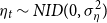 $\eta _t \sim NID(0, \sigma _\eta ^2)$
. Moreover, individuals are classified into two skill groups corresponding to educational attainment, denoted by
 $\iota \in \{h, l\}$
for high- and low-skilled individuals, respectively. All individuals maximize expected lifetime utility by choosing labor supply (
 $h_{i,j}$
), savings
 $(a_{i,j})$
, and consumption
 $(c_{i,j})$
:
 \begin{equation} u(c_{i,j}, h_{i,j})+\sum _{s=1}^{J-j+1} \beta ^s \prod _{q=1}^s (\psi _q)u(c_{i,s+1}, h_{i,s+1}), \end{equation}
where
 $\beta$
is the time discount factor and
 $\psi _q$
denotes the probability of survival to age
 $j+1$
conditional on being alive at age
 $j$
.
2.2 Technology
Aggregate production follows a constant-returns-to-scale Cobb–Douglas technology:
 \begin{equation} F(K_t, N_t)=A_tK_t^\alpha N_t^{1-\alpha }, \end{equation}
where
 $\alpha$
is the capital share of the output;
 $K_t$
is the aggregate capital shock;
 $N_t$
is the aggregate labor. The firm maximizes its profit in every period:
 \begin{equation*}\Pi _t(K_t, N_t)=Y_t-w_tN_t-(r_t+\delta )K_t.\end{equation*}
The first-order conditions yield the standard factor pricing equations, equating factor prices to marginal products:
 \begin{equation} \begin{split} w_t&=A_t(1-\alpha )k_t^\alpha ,\\[3pt] r_t&=A_t\alpha k_t^{\alpha -1}-\delta , \end{split} \end{equation}
where
 $k_t$
is the capital-labor ratio at time
 $t$
, and
 $\delta \lt 1$
is the depreciation rate of physical capital. The aggregate resource constraint is:
 \begin{equation} C_t+K_{t+1}-(1-\delta )K_t+G_t \leq A_t K_t^\alpha N_t^{1-\alpha }, \end{equation}
where
 $C_t$
denotes aggregate consumption and
 $G_t$
government expenditure.
2.3 Government policy
The government levies taxes on labor income, capital income, and consumption to fund its expenditure
 $G_t$
. Following Conesa et al. (Reference Conesa, Kitao and Krueger2009), the individual taxable labor income is defined as
 \begin{equation*}y^l_{i,j}\equiv w_t\omega _{i,j}h_{i,j}-0.5 \tau _{ss}\min \{w_t\omega _{i,j}h_{i,j}, \bar {y}\},\end{equation*}
where
 $\bar {y}$
denotes the maximum taxable labor income and
 $\tau _{ss}$
is the payroll tax rate.Footnote
8
Capital income is given by
 $y^k \equiv r_t(a+beq_t)$
. Total taxes consist of four components: a nonlinear tax schedule
 $T(\! \cdot \!)$
on labor income
 $y^l_{i,j}$
, a flat tax rate
 $\tau _k$
on capital income
 $y^k_{i,j}$
, a flat tax rate
 $\tau _c$
on consumption
 $c_{i,j}$
, and an endogenous flat tax rate
 $\tau _I$
on total taxable income
 $I_{i,j}\equiv y^l_{i,j}+y^k_{i,j}$
.Footnote
9
The total tax liability at age
 $j$
is:
 \begin{equation} T_j=T\big(y^l_{i,j} \big)+\tau _k \big(y^k_{i,j}\big)+\tau _c (c_{i,j})+\tau _I (I_{i,j}). \end{equation}
To make the fiscal closure explicit: the following instruments are held fixed at their benchmark calibrated values throughout all experiments: government expenditure
 $G$
, social security benefits
 $SS$
, the payroll tax rate
 $\tau _{ss}$
, the capital income tax rate
 $\tau _k$
, and the progressive labor income tax schedule
 $T(\! \cdot \!)$
. The flat income tax rate
 $\tau _I$
is the sole endogenous fiscal instrument, adjusting to clear the government budget constraint (11) as
 $\tau _c$
varies. This design isolates the substitution of the consumption tax for the income tax, which is the central question of the paper, and follows the approach of Kitao (Reference Kitao2011) and Ventura (Reference Ventura1999).
In addition, the government operates a pay-as-you-go social security system, collecting payroll taxes and redistributing benefits
 $SS_t$
to retirees. The payroll tax paid by each individual is
 $\tau _{ss}\min \{w_t\omega _{i,j}h_{i,j},\bar {y}\}$
.
2.4 Equilibrium definition
In this section, we formally define the competitive equilibrium of this model. The state variables are individual assets
 $a$
, idiosyncratic productivity
 $\omega$
, and age
 $j$
, which are jointly represented as
 $\Omega _t=(j, a_t, \omega _t)$
, denoting the aggregate state of the economy at time
 $t$
.
Definition 1.
Given a sequence of human capital accumulation parameters
 $\{\Theta _j\}_{j=20}^{j_r-1}$
,Footnote
10
payroll tax rate
 $\{\tau _{ss}\}_{t=1}^\infty$
, capital income tax rate
 $\{\tau _k\}_{t=1}^\infty$
, consumption tax rate
 $\{\tau _{c}\}_{t=1}^\infty$
, government expenditure
 $\{G_t\}_{t=1}^\infty$
, social security benefits
 $\{SS_t\}_{t=1}^\infty$
, and demographic parameters
 $\{n, \psi _j\}$
; a tax function
 $T \, : \, \mathbb{R}_+ \rightarrow \mathbb{R}_+$
; a maximum taxable income for social security
 $\bar {y}$
; a production plan for the firm
 $(N, K)$
; an age-specific human capital accumulation function
 $S \, : \, \mathbb{R}_+ \times \mathbb{R}_+ \times \mathbb{R}_+ \rightarrow \mathbb{R}_+$
; and a utility function
 $U \, : \, \mathbb{R}_+ \times \mathbb{R}_+ \rightarrow \mathbb{R}_+$
: a stationary competitive equilibrium consists of individual decision rules
 $\{c, h\}$
for each state
 $\kappa$
, factor prices
 $\{w, r\}$
, accidental bequests
 $beq$
, and a stationary distribution of individuals
 $\{\mu (\kappa )\}$
such that the following conditions hold:
-
1. Each individual maximizes Equation (4) given prices
 $\{w, r\}$
, policy
$\{T\}$
, accidental bequests
$\{beq\}$
, benefits
$\{SS\}$
, and idiosyncratic productivity
$\{\omega \}$
subject to
(9)for
\begin{equation} \begin{split} c+a'=&w\omega h-\tau _{ss}w\omega h+(1+r)(a+beq)\\[3pt] &-T[w\omega h-0.5\tau _{ss}\min \{w\omega h, \bar {y}\}]-\tau _kr(a+beq)-\tau _c c \\[3pt] &-\tau _I [w\omega h-\tau _{ss}w\omega h+r(a+beq)], \end{split} \end{equation}
$j\leq j_r$
, and
(10)for
\begin{equation} \begin{split} c+a'=&SS+(1+r)(a+beq)\\[3pt] &-\tau _kr(a+beq)-\tau _c c -\tau _I [r(a+beq)] , \end{split} \end{equation}
$j \gt j_r.$
Individuals face the standard non-negativity and time constraints:
\begin{equation*}c \geq 0, 0 \leq h \leq 1, a\geq 0, a_1=0.\end{equation*}
-
2. The firm maximizes its profit according to 4 where prices
$w,r$
satisfying
and
\begin{equation*}r=\alpha A \left(\frac {K}{N} \right)^{\alpha -1}-\delta \end{equation*}
\begin{equation*}w=(1-\alpha )A \left(\frac {K}{N}\right)^\alpha .\end{equation*}
-
3. The social security system satisfies
\begin{equation*}\tau _{ss}=\frac {\sum _{j \gt j_r} SS \mu (\kappa )}{\sum _{j\leq j_r} \min \{w\omega h, \bar {y}\} \mu (\kappa )}.\end{equation*}
-
4. Accidental bequests are determined by
\begin{equation*}beq=\sum (1-\psi )a'\mu (\kappa ).\end{equation*}
-
5. Government budget balance requires
(11)
\begin{equation} \begin{split} G=&\sum \tau _k[r(a+beq)]\mu (\kappa )+\sum _{j\leq j_r}T[w\omega h-0.5\tau _{ss} \min \{w\omega h, \bar {y}\})]\mu (\kappa )+\tau _c \sum c \mu (\kappa )\\[3pt] &+\tau _I \Bigg \{\sum _{j \leq j_r}[w\omega h-0.5\tau _{ss}\min \{w\omega h, \bar {y}\})]\mu (\kappa )+\sum [r(a+beq)]\mu (\kappa )]\Bigg \}. \end{split} \end{equation}
-
6. The markets for capital and labor clear:
and the aggregate resource constraint holds:
\begin{align*} \begin{split} K &=\sum a \mu (\kappa ) \\[3pt] N &=\sum \omega h \mu (\kappa ), \end{split} \end{align*}
\begin{equation*}\sum c \mu (\kappa )+\sum a' \mu (\kappa )+G=AK^\alpha N^{1-\alpha }+(1-\alpha )K.\end{equation*}
-
7. The distribution
$\mu (\kappa )$
is stationary, satisfying the law of motion
$\mu (\kappa )=Q_\mu \mu (\kappa )$
, where
$Q_\mu$
is a one-period recursive operator on the distribution.




3. Calibration
We calibrate the model to replicate key features of the U.S. economy. A subset of parameters is directly drawn from established empirical studies and previous literature, while the remaining parameters are internally calibrated to match the baseline steady-state equilibrium to U.S. data moments. Table 1 reports externally assigned parameters and Table 2 summarizes the internally calibrated parameters.
External parameters

Table 1. Long description
A table with six rows and four columns detailing external parameters used for model calibration. The columns are labeled Parameter, Value, Source, and include grouped rows under headings like Demographics, Firm parameters, Productivity parameters, Government parameters, and Human capital parameters. Row 1: Demographics, Retire age, 66, By assumption. Row 2: Demographics, Max age, 100, By assumption. Row 3: Demographics, Sur. prob, Bell and Miller (2005). Row 4: Demographics, Pop. growth, 1.1 percent, Peterman (2016). Row 5: Firm parameters, Capital share, 0.36, Peterman (2016). Row 6: Firm parameters, Depreciation rate, 8.33 percent, Peterman (2016). Row 7: Firm parameters, Technology, 1, Normalization. Row 8: Productivity parameters, Persistence shock, 0.017, Kaplan (2012). Row 9: Productivity parameters, Persistence, 0.958, Kaplan (2012). Row 10: Productivity parameters, Permanent shock, 0.065, Kaplan (2012). Row 11: Productivity parameters, Transitory shock, 0.081, Kaplan (2012). Row 12: Government parameters, Payroll tax, 0.124, Conesa et al. (2009). Row 13: Government parameters, Avg. tax rate, 0.911, Guner et al. (2016). Row 14: Government parameters, Tax progressivity, 0.053, Guner et al. (2016). Row 15: Human capital parameters, 0.407, Chang et al. (2002). Row 16: Human capital parameters, 0.326, Chang et al. (2002).
Calibration parameters
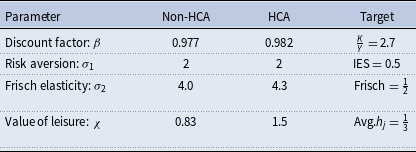
Table 2. Long description
A table comparing calibration parameters for Non-HCA and HCA models. The table has 5 rows and 4 columns. Column headers are Parameter, Non-HCA, HCA, and Target. Row 1: Discount factor: β, 0.977, 0.982, κ/η = 2.7. Row 2: Risk aversion: σ1, 2, 2, IES = 0.5. Row 3: Frisch elasticity: σ2, 4.0, 4.3, Frisch = 1/2. Row 4: Value of leisure: χ, 0.83, 1.5, Avg.hj = 1/3.
3.1 Demographics
We assume individuals enter the labor force at age 20, retire at age 66, and may live up to age 100. The conditional survival probabilities
 $\psi _j$
follow the estimates of Bell and Miller (Reference Bell and Miller2005), and the population growth rate is set at 1.1% in line with Peterman (Reference Peterman2016).
3.2 Preferences and endowments
The instantaneous utility function is specified as
 \begin{equation*}u(c_t, 1-h_t)=\frac {c_t^{1-\sigma _1}}{1-\sigma _1}+\chi \frac {(1-h_t)^{1-\sigma _2}}{1-\sigma _2}, \end{equation*}
where
 $\chi$
is a preference weight on leisure, calibrated to match the average working hours target,
 $\sigma _1$
is the coefficient of relative risk aversion for consumption, and
 $\sigma _2$
governs the curvature of the leisure component and determines the Frisch elasticity of labor supply.
The discount factor
 $\beta$
is calibrated to match the target capital-output ratio of 2.7, and the risk aversion parameter
 $\sigma _1$
is set to 2 following Conesa et al. (Reference Conesa, Kitao and Krueger2009). We set
 $\sigma _2=4$
in the non-HCA model and
 $\sigma _2=4.3$
in the HCA model so that the average Frisch elasticity of labor supply equals
 $\frac {1}{2}$
, consistent with Peterman (Reference Peterman2016).Footnote
11
The parameter
 $\chi$
is calibrated such that agents on average spend one-third time endowment working.
3.3 Idiosyncratic labor productivity
Each individual is endowed with one unit of productive time that can be allocated between labor supply (
 $h_{i,j}$
) and leisure (
 $1-h_{i,j}$
). The idiosyncratic labor productivity
 $\omega _{i,j}$
depends on the age
 $j$
, age-specific human capital
 $\varepsilon$
, innate ability
 $\zeta$
, skill level
 $\iota$
, and an idiosyncratic shock
 $\eta$
. The idiosyncratic shock
 $\eta$
takes seven discrete values for each skill level, where the first five shocks,
 $\eta _{\iota ,1}, \eta _{\iota ,2}, \ldots , \eta _{\iota ,5}$
are “normal” productivity shocks generated by a standard AR(1) process. The last two shocks,
 $\eta _{\iota ,6}, \eta _{\iota ,7}$
represent rare high-productivity states (“lucky states”) not captured in the PSID data (Kindermann and Krueger (Reference Kindermann and Krueger2022)). To better replicate the observed U.S. wealth Gini, we extend the original
 $5 \times 5$
Markov transition matrix to a
 $7 \times 7$
matrix by incorporating these two extreme states following Kindermann and Krueger (Reference Kindermann and Krueger2022):
 \begin{equation*} \pi _\iota = \begin{bmatrix} \pi _{11,\iota }(1-\pi _{6,\iota }) &\quad\ldots &\quad\pi _{13,\iota }(1-\pi _{6,\iota }) &\quad\ldots &\quad\pi _{15,\iota }(1-\pi _{6,\iota }) &\quad \pi _{6,\iota }&\quad 0\\[3pt] \vdots &\quad\vdots &\quad\vdots &\quad\vdots &\quad\vdots &\quad\vdots &\quad\vdots \\[3pt] \pi _{51,\iota }(1-\pi _{6,\iota })&\quad\ldots &\quad\pi _{53,\iota }(1-\pi _{6,\iota }) &\quad\ldots &\quad\pi _{55,\iota }(1-\pi _{6,\iota }) &\quad\pi _{6,\iota } &\quad 0 \\[3pt] 0&\quad\ldots &\quad1-\pi _{66,\iota }-\pi _{67,\iota } &\quad\ldots &\quad0 &\quad\pi _{66,\iota } &\quad\pi _{67,\iota } \\[3pt] 0&\quad\ldots &\quad0 &\quad\ldots &\quad0 &\quad1-\pi _{77,\iota } &\quad\pi _{77,\iota } \end{bmatrix} \end{equation*}
For each normal state
 $\{\eta _{\iota ,1}, \eta _{\iota ,2}, \ldots , \eta _{\iota ,5}\}$
, there exists a small probability of transitioning to
 $\eta _{\iota ,6}$
. Transitioning to the highest shock
 $\eta _{\iota ,7}$
requires first reaching
 $\eta _{\iota ,6}$
. These “lucky states” are temporary: upon receiving a negative shock, the agent reverts to
 $\eta _{\iota ,3}$
.
The persistent, permanent, and transitory components of idiosyncratic labor productivity are calibrated following Kaplan (Reference Kaplan2012). These shocks are normally distributed with zero mean, with variances
 $\sigma _\zeta ^2=0.065, \sigma _\upsilon ^2=0.017$
, and
 $\sigma _\eta ^2=0.081$
, respectively, and the persistent parameter is
 $\rho =0.958$
.
3.4 Technology
Following Peterman (Reference Peterman2016), the capital share,
 $\alpha$
, is set to 0.36. Level of technology
 $A$
is normalized to one. The depreciation rate,
 $\delta$
, is set to 8.33% to target the observed investment output ratio of 25.5%.
3.5 Government policy
We adopt the income tax function of Benabou (Reference Benabou2002) to capture the progressive structure of the U.S. income tax system:
 \begin{equation} T_t(y_t)=y_t-\lambda _0 (y_t)^{1-\lambda _1}. \end{equation}
Here,
 $\lambda _0$
determines the average tax rate, and
 $\lambda _1$
governs the curvature of the tax function, i.e. the progressivity of the system, with
 $1-\lambda _1$
representing the elasticity of post-tax to pre-tax income (Heathcote et al. (Reference Heathcote, Storesletten and Violante2017)). Following the estimates of Guner et al. (Reference Guner, Lopez-Daneri and Ventura2016), we set
 $\lambda _0=0.911$
and
 $\lambda _1=0.053$
based on U.S. data.
4. Results
4.1 Benchmark results
In this section, we present the benchmark results for both the HCA and the non-HCA models. These two benchmark models are calibrated separately to match the target moments described in Section 3 (see Table 2). Table 3 presents the aggregate economic variables for both models. Although slight differences exist between the two models, the benchmark results are quantitatively close. Both models serve as baseline frameworks for the subsequent experiments. In addition, both models generate Gini coefficients that are broadly consistent with U.S. data (see Table 4). Specifically, the labor income, consumption, and disposable income Gini coefficients are closely aligned with empirical estimates. However, generating realistic wealth Gini coefficients remains challenging. To improve the credibility of the wealth Gini estimates, we adopt the calibration approach of Kindermann and Krueger (Reference Kindermann and Krueger2022). The resulting wealth Gini coefficients are 0.70 for the HCA model and 0.77 for the non-HCA model. Both are considerably closer to the empirical estimate of 0.80 than the values of 0.63 reported in Guner et al. (Reference Guner, Lopez-Daneri and Ventura2016) and 0.60 reported in Ventura (Reference Ventura1999).
Aggregate economic variables

Table 3. Long description
A table comparing aggregate economic variables between Non-HCA and HCA models. The table has 12 rows and 3 columns. Column headers are Non-HCA and HCA. Row labels are Aggregate, Y, K, N, Avg. hours, w, r, beq, Average tax rate, Labor, Capital, Ratio, Marginal tax rate, Labor, Capital, Ratio. Row 1: Non-HCA, 1.19; HCA, 1.17. Row 2: Non-HCA, 3.17; HCA, 3.24. Row 3: Non-HCA, 0.68; HCA, 0.68. Row 4: Non-HCA, 0.33; HCA, 0.30. Row 5: Non-HCA, 0.93; HCA, 0.91. Row 6: Non-HCA, 0.052; HCA, 0.046. Row 7: Non-HCA, 0.040; HCA, 0.039. Row 8: Non-HCA, 0.1259; HCA, 0.1232. Row 9: Non-HCA, 0.0976; HCA, 0.0848. Row 10: Non-HCA, 1.2897; HCA, 1.4539. Row 11: Non-HCA, 0.1723; HCA, 0.1697. Row 12: Non-HCA, 0.1455; HCA, 0.1333. Row 13: Non-HCA, 1.1841; HCA, 1.2734.
Gini coefficients

Table 4. Long description
A table comparing Gini coefficients for different economic variables across data, non-HCA model, and HCA model. The table has four rows and four columns. Column headers are Data, Non-HCA model, and HCA model. Row labels are Labor income, Consumption, Disposable income, and Wealth. Row 1: Data, 0.55; Non-HCA model, 0.53; HCA model, 0.52. Row 2: Data, 0.34; Non-HCA model, 0.33; HCA model, 0.31. Row 3: Data, 0.40; Non-HCA model, 0.39; HCA model, 0.36. Row 4: Data, 0.80; Non-HCA model, 0.77; HCA model, 0.70.
Note: The U.S. data is based on the data for 1999–2013 taken from Fisher et al. (Reference Fisher, Johnson, Latner, Smeeding and Thompson2016).
Next, we compare the benchmark results of both models against the actual data by plotting the life-cycle profiles. Figure 1 shows the average time devoted to work, average consumption, median savings, and average labor income for both models compared to the actual data. The red, blue, and dashed lines represent the trends in the HCA model, the non-HCA model, and the actual data, respectively.Footnote 12
Labor supply exhibits a hump-shaped pattern in the data whereas the models produce a monotonically decreasing profile with a higher initial level. This occurs because young individuals enter the model economy without assets and must work to consume and accumulate precautionary savings. As individuals accumulate experience and wealth, they gradually reduce working hours. In reality, individuals receive parental support or inheritances and can borrow for consumption, which leads to a lower initial labor supply. Conversely, middle-aged workers often face childcare and eldercare responsibilities, explaining the higher observed labor supply between ages 30 and 60. Noticeably, upon reaching retirement age, HCA working hours decline more than non-HCA working hours, as diminishing returns to human capital raise the Frisch elasticity.
Actual, non-HCA and HCA life-cycle profiles.

The consumption profiles in both models and the data display hump-shaped patterns. Model-generated consumption levels are generally higher than those observed in the PSID data, as the latter only records food expenditures, whereas the models include all consumption categories. Consumption in the data peaks around age 45 while it peaks near retirement (age 66) in the model. This difference reflects that the data exclude non-durable and luxury goods. Consequently, the data show a decline in food consumption after age 45, whereas the model captures total consumption that remains high until retirement. After age 66, consumption drops sharply as individuals retire in the model. Additionally, the working-age consumption profile in the HCA is slightly steeper than in the non-HCA. The consumption profiles are consistent with those in Conesa et al. (Reference Conesa, Kitao and Krueger2009).
Savings exhibit similar hump-shaped profiles across models and data, peaking around age 66. In both models, savings increase during working years and decline after retirement. Actual savings in the data exceed model predictions between ages 50 and 60, likely due to intergenerational transfers or inheritances. In the data, savings after age 70 remain stable or slightly increase, reflecting altruistic motives, then decline after age 85 which is the same trend in the model.
Labor income profiles in both models and the data align closely before age 55. The data generally display a hump-shaped pattern, whereas both models predict an increasing trend in labor income before retirement. This discrepancy arises because all modeled individuals are required to work until age 66 (unless they die earlier), while in reality, individuals near age 60 often reduce their working hours or transition to part-time work. The Non-HCA earnings profile exhibits a relatively flat or moderately hump-shaped pattern, peaking around middle age before gradually declining. In contrast, the HCA profile shows a steeper increase during early working years, reaching a higher peak, and often maintaining elevated earnings until closer to retirement, reflecting the returns on human capital investment. The divergence between the HCA and non-HCA profiles after age 40–50 highlights the role of human capital in sustaining earnings growth and delaying peak earnings.
Overall, the baseline results in both models reasonably replicate the empirical life-cycle patterns of labor supply, income, consumption, and savings. The shapes of the labor supply and savings profiles are similar to those in Peterman (Reference Peterman2016), but our models provide a better fit for savings and young-age labor income. The most significant departure from Peterman (Reference Peterman2016) lies in the consumption profile: our baseline models more accurately capture the sudden decline in consumption upon retirement.
4.2 Proportional consumption tax experiments
In this section, we explore the implications of replacing the income tax with a proportional consumption tax on aggregate macroeconomic outcomes, social welfare, and inequality. Specifically, we quantitatively analyze the effects of increasing the consumption tax rate from 5% to 95% in 10-percentage-point increments in both models, while keeping all other parameters and government expenditure fixed at their benchmark levels. To maintain fiscal neutrality, the income tax rate is correspondingly reduced, and may become negative to offset the additional consumption tax revenue.
4.2.1 Macroeconomic effects
Figures 2 and 3 show how savings, consumption, the interest rate, labor supply, the wage, and output change as the consumption tax rate increases in the HCA model (red line) and the non-HCA (blue line) model.
Capital, consumption, transfer, and interest rate.

labor supply, working hours, wage rate, and output.

Both models exhibit an increase in the capital stock. For consumption tax rates below 55%, the changes in the capital stock are virtually identical across the two models. However, once the tax rate exceeds 55%, the capital stock in the HCA model rises substantially faster and reaches a significantly higher level than that in the non-HCA model. Similarly, aggregate transfers (comprising accidental bequests and social security transfers) begin to diverge once the consumption tax rate surpasses 55%. Both models show increasing transfers for tax rate below 65%, but beyond this threshold, transfers start to decline. In the HCA model, the decline is more gradual, and transfers remain higher than those in the non-HCA model.
Aggregate consumption in both models follows a hump-shaped pattern. The differences between the two models are relatively modest: at lower consumption tax rates, aggregate consumption in the HCA model is slightly lower than in the non-HCA model, whereas at higher rates, the opposite holds. In both models, the interest rate first decreases and then increases, following a similar trajectory. The turning point again occurs at a consumption tax rate of approximately 55%.Footnote 13
Aggregate labor supply (shown in the upper-left panel of Figure 3), total working hours, average income, and output all increase with the consumption tax rate. The figure shows that working hours remain relatively stable at tax rates below 50% but rise sharply once the rate exceeds 55%. Intuitively, individuals work longer to offset the heavier consumption tax burden. Moreover, individuals in the HCA model work fewer hours than those in the non-HCA model, even though the slopes of the working-hours curves are similar. This suggests that endogenous human capital accumulation reduces total labor hours but does not alter the responsiveness of hours to consumption tax changes. Nevertheless, the aggregate labor supply responses differ across the two models at tax rates below 55%, which is consistent with the observed differences in average income.
In Figure 4, the capital–output ratio, transfer–output ratio, and capital–labor ratio all exhibit hump-shaped patterns, peaking at a consumption tax rate of about 55%. These ratios are highly similar across the HCA and non-HCA models. Once the tax rate exceeds 55%, all three ratios begin to decline. Consequently, the interest rate in Figure 2 displays a U-shaped pattern, reaching its minimum at approximately 55% in both models. Although the capital stock, labor supply, and output all increase when the consumption tax rate exceeds 55%, the declines in the capital–output and capital–labor ratios indicate that output and labor supply grow faster than the capital stock. The reduction in the transfer–output ratio reflects the combined effect of lower aggregate transfers and higher output. Moreover, these ratios are slightly higher in the HCA model when the tax rate exceeds 55%. Intuitively, endogenous human capital accumulation allows individuals to enhance their labor productivity more rapidly, accelerating the growth of production, labor supply, average income, and capital accumulation.
Capital output ratio, capital labor ratio, and capital labor ratio.

In brief, as the consumption tax rate increases, individuals face stronger incentives to work, save, and invest. Consequently, labor supply, aggregate savings, and output all rise. Consumption first increases and then declines, while the interest rate initially falls and later rises, with a turning point for both at around 55%. These results are consistent with Kitao (Reference Kitao2011) and Ventura (Reference Ventura1999). Specifically, Kitao (Reference Kitao2011) finds that when the consumption tax rate rises from 5% to 45%, the capital stock, labor supply, consumption, and wages all increase, whereas the interest rate declines. Similarly, Ventura (Reference Ventura1999) reports that replacing an income tax system with a flat consumption tax leads to increases in the capital stock, labor supply, and savings.Footnote 14
Our results diverge from those of Nakajima and Takahashi (Reference Nakajima and Takahashi2020), who employs an infinite-horizon model with both divisible and indivisible labor. Focusing on the divisible labor case, that study finds that higher consumption taxes reduce labor supply, output, and the capital–output ratio. In contrast, our model predicts increases in these aggregates, driven by differences in tax structure and the finite life cycles. Our findings also depart from those of Correia (Reference Correia2010), who reports that raising a flat consumption tax improves labor efficiency,Footnote 15 whereas we observe the opposite effect for tax rates below 30%. Importantly, in Correia (Reference Correia2010), labor and capital income tax rates are simultaneously reduced until they are fully replaced by the consumption tax.
Unlike Ventura (Reference Ventura1999), Correia (Reference Correia2010), Kitao (Reference Kitao2011), and Nakajima and Takahashi (Reference Nakajima and Takahashi2020), our framework incorporates endogenous human capital accumulation. In the HCA model, human capital evolves each period endogenously, shaping labor productivity, average income, output, and transfers. These dynamics, in turn, affect individuals’ decisions regarding hours worked, savings, and consumption. Consequently, economic aggregates in the HCA model are more sensitive to changes in the consumption tax rate, particularly at higher tax levels. As a result, we observe steeper responses in the HCA model relative to the non-HCA model when the tax rate exceeds 55%.
Three mechanisms drive the differential response of the HCA model. First, the Frisch elasticity of labor supply increases much more sharply with age in the HCA model than in the non-HCA model, where it remains relatively flat: young workers internalize that current labor effort raises future wages, making them less elastic to tax changes early in life. Second, unlike an income tax, a consumption tax does not reduce the after-tax payoff to building human capital. Replacing income taxation with consumption taxation therefore removes an additional distortion in the HCA model that is entirely absent in the non-HCA model, producing a stronger aggregate efficiency gain. Third, because endogenous human capital amplifies the responses of wages and productivity, the HCA model exhibits steeper aggregate responses at higher consumption tax rates. We provide a formal analytical illustration of these mechanisms in Section B.
Our results also contrast with Conesa et al. (Reference Conesa, Li and Li2020), who find welfare losses from switching fully from income to consumption taxation. Their model is an infinite-horizon economy with no life-cycle structure and no human capital; progressivity is achieved through differentiated rates on basic versus non-basic goods rather than through expenditure-level brackets. The contrasting findings reflect both the different research question (full income tax replacement versus revenue-neutral rate changes) and the absence of human capital and life-cycle dynamics in their framework. We view our results as complementary: at moderate, revenue-neutral rates, consumption tax reform generates welfare gains that become further amplified under a well-designed progressive structure.
4.2.2 Inequalities and welfare effects
Figure 5 plots the inequality measures for both the HCA (red line) and non-HCA (blue line) models as the consumption tax rate increases. The wealth Gini generally declines, the consumption Gini rises, the labor income (earnings) Gini follows a U-shaped pattern (first decreasing and then increasing), and the disposable income Gini first increases and then falls. These patterns contrast with those in Nakajima and Takahashi (Reference Nakajima and Takahashi2020), where the wealth and labor income Ginis increase, while the consumption and disposable income Ginis decline.
In both models, low-income individuals respond to higher consumption taxes by increasing precautionary savings, working more, and consuming less. In contrast, high-income individuals, who are less liquidity constrained, reduce their consumption only slightly. Consequently, wealth inequality declines (a lower wealth Gini), while consumption inequality rises (a higher consumption Gini).
Gini coefficients of wealth, consumption, labor income, and disposable income.

As the consumption tax rate continues to rise, both income groups increase their labor supply. But the pattern of adjustment differs below and above the 55% threshold. Below that threshold, low-income households expand working hours substantially, whereas high-income households adjust little.Footnote 16 Consequently, the labor income Gini declines, indicating narrower earnings inequality. Accounting for progressive labor income taxation and transfer mechanisms, the disposable income of low-income individuals grows more slowly than their labor income,Footnote 17 while that of high-income individuals remains relatively stable. This widens the disposable income gap and pushes up the disposable income Gini for tax rate below 55%. Beyond that threshold, both groups increase working hours significantly, but the higher labor productivity of rich households amplifies earnings inequality. Meanwhile, progressive taxation helps compress disposable income disparities, causing the disposable income Gini to fall.
Overall, the earnings and disposable income Ginis move in opposite directions, consistent with Nakajima and Takahashi (Reference Nakajima and Takahashi2020). The lower Gini levels in the HCA model (red line) reflect lower benchmark inequality. We therefore focus on relative changes (that is, the slopes of the Gini coefficients) when comparing the two models. Inequality responses are more pronounced in the HCA model, as indicated by steeper slopes. Endogenous human capital accumulation enables individuals to raise their productivity through work, which boosts labor income and shapes savings and consumption decisions. Consequently, incorporating human capital accumulation amplifies the responsiveness of both economic aggregates and inequality measures to consumption tax reforms.
Social welfare as measured by % change in CEV.

We evaluate welfare using the consumption equivalent variation (CEV), defined as the constant percentage change in consumption that equates discounted lifetime utilities between the baseline and reformed economies:
 \begin{equation*}CEV=\left (\frac {V_e}{V_b}\right )^\frac {1}{1-\sigma _1}-1\end{equation*}
where
 $V_e$
and
 $V_b$
denote the value functions of the experiment and the baseline, respectively.
Increasing the consumption tax rate generates a hump-shaped pattern in CEVs. As shown in Figure 6, both models indicate welfare gains when the tax rate is below 45%, consistent with Kitao (Reference Kitao2011). However, once the rate exceeds 55%, welfare declines sharply. This hump-shaped welfare response parallels the hump-shaped path of aggregate consumption (Figure 2). The welfare decline beyond 55% is partly driven by the increasing disutility of additional work hours.
When comparing the two models, the HCA model consistently yields higher CEVs, implying smaller welfare losses at higher consumption tax rates. Endogenous human capital accumulation allows individuals to achieve greater productivity with fewer working hours, thereby enabling more leisure and higher utility relative to the non-HCA model.
In brief, raising the consumption tax rate enhances welfare when the rate remains below 55%, but leads to welfare losses once this threshold is surpassed. Although higher consumption tax rates mitigate wealth inequality, they simultaneously intensify consumption inequality. The HCA model exhibits greater sensitivity to changes in the consumption tax rate, as reflected in the steeper responses of inequality measures, driven by the inclusion of human capital accumulation.
4.3 Progressive consumption tax experiments
This section quantitatively examines the effects of transforming the proportional consumption tax into a progressive system. We first introduce an exemption threshold, creating a structure analogous to the Hall–Rabushka flat tax (Hall and Rabushka, Reference Hall and Rabushka1995). We then extend the framework to a three-bracket, piecewise linear consumption tax to explore the economic implications of varying degrees of progressivity.
4.3.1 A consumption tax with an exemption
We specify an exemption threshold,
 $c_m$
, which represents the subsistence level of consumption. Consumption below this threshold is tax-exempt, ensuring that essential needs remain untaxed. A flat tax rate applies to the portion of consumption exceeding the exemption level. The consumption tax function is given by
 \begin{equation} T(c) = max\left \{\tau _{c}(c-c_m), 0\right \} \end{equation}
where
 $T(c)$
denotes the consumption tax function, and
 $\tau _c$
is the marginal tax rate applied to consumption above the threshold. We fix
 $\tau _c$
at its benchmark value of 5% and consider three alternative exemption thresholds,
 $c_m \in \{0.3, 0.5, 0.7\}$
. An increase in
 $c_m$
implies a greater degree of tax progressivity.
Tables 5 and 6 show that raising the exemption threshold reduces total output, the capital stock, and bequests, while increasing aggregate labor supply. This simultaneous decline in capital and rise in labor lowers the capital–labor ratio, leading to a lower wage rate and a higher interest rate. Overall, the reforms narrow consumption inequality but widen wealth inequality.
A consumption tax with an exemption

Table 5. Long description
A table comparing economic indicators under different consumption tax exemption thresholds. The table has 18 rows and 10 columns. Column headers are HCA, Baseline, c_m = 0.3, % change, c_m = 0.5, % change, c_m = 0.7, % change. Row labels include Aggregate, Y, K, N, Avg. hours, w, r, beq, CEV, Gini, Consumption, Wealth, Average tax rate, Labor, Capital, Ratio, Marginal tax rate, Labor, Capital, Ratio. Row 1: HCA, Baseline, c_m = 0.3, % change, c_m = 0.5, % change, c_m = 0.7, % change. Row 2: Aggregate, 1.17, 1.17, 0.2, 1.16, 1.2, 1.15, 1.6. Row 3: Y, 3.14, 3.13, 0.3, 3.03, 3.5, 2.95, 6.1. Row 4: K, 0.67, 0.67, 0.1, 0.67, 0.2, 0.68, 1.1. Row 5: Avg. hours, 0.30, 0.30, 0.5, 0.30, 0.6, 0.30, 0.1. Row 6: w, 0.91, 0.91, 0.3, 0.90, 1.2, 0.90, 1.6. Row 7: r, 0.051, 0.051, 0.4, 0.054, 6.9, 0.057, 12.7. Row 8: beq, 0.037, 0.037, 0.2, 0.036, 5.2, 0.034, 8.3. Row 9: CEV, 0.37%, 1.02%, 2.07%. Row 10: Gini, Consumption, 0.31, 0.31, 0.3, 0.30, 1.3, 0.30, 2.4. Row 11: Wealth, 0.69, 0.68, 0.1, 0.70, 1.9, 0.69, 0.2. Row 12: Average tax rate, Labor, 0.1245, 0.1246, 0.1252, 0.1258. Row 13: Capital, 0.0861, 0.0862, 0.0877, 0.0874. Row 14: Ratio, 1.4450, 1.4457, 1.4278, 1.4392. Row 15: Marginal tax rate, Labor, 0.1709, 0.1710, 0.1716, 0.1721. Row 16: Capital, 0.1346, 0.1346, 0.1361, 0.1358. Row 17: Ratio, 1.2697, 1.2702, 1.2611, 1.2678.
A consumption tax with an exemption (cont.)

Table 6. Long description
A table comparing economic indicators under different consumption tax exemption scenarios. The table has 18 rows and 10 columns. Column headers are Baseline, c_m = 0.3, % change, c_m = 0.5, % change, c_m = 0.7, % change, and row labels are Aggregate Y, K, N, Avg. hours, w, r, beq, CEV, Gini Consumption, Wealth, Average tax rate Labor, Capital, Ratio, Marginal tax rate Labor, Capital, Ratio. Row 1: Aggregate Y, 1.18, 1.18, 0.2, 1.17, 1.3, 1.17, 1.7. Row 2: K, 3.17, 3.15, 0.4, 3.04, 4.1, 2.96, 6.6. Row 3: N, 0.68, 0.68, 0.1, 0.69, 0.3, 0.69, 1.1. Row 4: Avg. hours, 0.33, 0.33, 0.8, 0.33, 0.5, 0.34, 0.2. Row 5: w, 0.93, 0.92, 0.2, 0.91, 1.3, 0.91, 1.7. Row 6: r, 0.052, 0.052, 0.5, 0.056, 7.6, 0.059, 13.5. Row 7: beq, 0.040, 0.040, 0.4, 0.038, 5.0, 0.037, 6.9. Row 8: CEV, 0.07%, 0.82%, 2.01%. Row 9: Gini Consumption, 0.34, 0.34, 0.3, 0.33, 1.4, 0.33, 2.2. Row 10: Wealth, 0.76, 0.76, 0.05, 0.77, 1.8, 0.76, 0.7. Row 11: Average tax rate Labor, 0.1259, 0.1261, 0.1264, 0.1265. Row 12: Capital, 0.0976, 0.0977, 0.0999, 0.0999. Row 13: Ratio, 1.2897, 1.2916, 1.2652, 1.2670. Row 14: Marginal tax rate Labor, 0.1723, 0.1724, 0.1727, 0.1728. Row 15: Capital, 0.1455, 0.1455, 0.1476, 0.1476. Row 16: Ratio, 1.1841, 1.1853, 1.1699, 1.1711.
These outcomes stem from the structural features of the reform. Greater progressivity (achieved through a higher exemption level) shifts the tax burden onto high-consuming, typically wealthier households. As a result, the share of consumption tax revenue in total fiscal receipts falls. To maintain budget balance, the proportional income tax rate must rise, increasing the income tax’s contribution to total revenue.
This fiscal reallocation triggers offsetting behavioral responses. The higher effective tax on capital discourages saving, leading to lower aggregate capital accumulation and smaller bequests. At the same time, the labor tax wedge narrows for households below the exemption threshold but widens for those above it. Consequently, average hours worked and total labor supply initially fall, but subsequently recover and exceed their benchmark levels as the exemption threshold rises further.
Crucially, the strong disincentive to save and invest outweighs the modest positive labor supply response. The net effect is a contraction in aggregate output and a decline in overall welfare. Thus, while the policy effectively reduces consumption inequality, it inadvertently amplifies wealth inequality.
In brief, transforming the proportional consumption tax into a progressive system by introducing an exemption threshold not only erodes the aggregate efficiency gains achieved under the benchmark scenario, but also exacerbates wealth inequality, ultimately leading to lower social welfare.
4.3.2 A three-bracket piecewise linear consumption taxes
To further enhance the progressivity of the consumption tax, we introduce an additional upper threshold,
 $c_h$
, as defined in Equation 13. This yields two thresholds,
 $c_m$
and
 $c_h$
, that divide consumption into three tax brackets: the lower bracket
 $[0, c_m)$
, the middle bracket
 $[c_m, c_h)$
, and the upper bracket
 $[c_h, \infty )$
. Each bracket is subject to a distinct linear tax rate: the lowest bracket is exempted (zero rate), the middle bracket is taxed at the lower rate,
 $\tau _{c_1}$
, and the upper bracket is taxed at the higher rate,
 $\tau _{c_2}$
, creating a more progressive structure. The resulting three-bracket piecewise linear consumption tax function is given byFootnote
18
 \begin{equation} T(c) = \begin{cases} 0 & \text{ if }\,\,\,\,\,\,\,\,\,c \lt c_m \\[3pt] \tau _{c_1}(c-c_m) & \text{ if } \,\,c_m \leq c \lt c_h \\[3pt] \tau _{c_2}(c-c_h) + \tau _{c_1}(c_h-c_m) & \text{ if }\,\,\,\,\,\,\,\,\,c \geq c_h, \end{cases} \end{equation}
where
 $\tau _{c_1} \leq \tau _{c_2}$
.
Progressive consumption taxes of this form can be implemented through several mechanisms discussed in the public finance literature. The most direct is the personal expenditure tax (Kaldor, Reference Kaldor1955): households compute taxable consumption as income minus net saving on their annual tax return, and progressive rates are applied to this figure. Since income data are already collected by tax authorities, the main additional requirement is the reporting of net saving through financial account disclosures. Costa and Santos (Reference da Costa and Santos2023) show that income averaging (using information already gathered by the social security system) can deliver approximately half the welfare gains of a full progressive consumption tax reform without comprehensive household expenditure tracking. A second approach is the X-Tax (Viard and Carroll, Reference Viard and Carroll2012), which applies a progressive household wage tax alongside a flat business cash-flow tax, achieving progressivity using wage records that payroll systems already collect. A third approach, already practiced in many countries, applies reduced or zero VAT rates to basic consumption goods such as food and medicine. Our three-bracket structure is designed to be administratively simple: a small number of brackets with flat rates within each bracket closely approximates a smooth progressive schedule while remaining tractable for tax authorities to administer.
In this analysis, we keep both thresholds fixed at
 $c_m=0.3$
and
 $c_h=0.9$
and examine how increasing consumption tax progressivity, by varying the tax rates across brackets, affects the economy. Specifically, we set the middle-bracket rate
 $\tau _{c_1}$
to 3%, 4%, or 5%, and the upper-bracket rate
 $\tau _{c_2}$
to 5%, 10%, or 15%. This yields nine counterfactual scenarios, corresponding to all combinations of the two rates.
We present the results for three experiments with
 $\tau _{c_1}=5\%$
and
 $\tau _{c_2} \in \{5\%, 10\%, 15\%\}$
. The results in the first two columns of Tables 7 and 8 are consistent with those reported in the analogous columns of Tables 5 and 6.Footnote
19
Holding
 $\tau _{c_1}$
fixed at 5% and increasing
 $\tau _{c_2}$
allows us to examine the effects of greater progressivity within the consumption tax framework.Footnote
20
A three-bracket piecewise linear consumption taxes

Table 7. Long description
A table comparing economic indicators under different tax scenarios. The table has 12 rows and 9 columns. Column headers are HCA, Baseline, 5 percent comma 5 percent, percent change, 5 percent comma 10 percent, percent change, 5 percent comma 15 percent, and percent change. Row labels include Aggregate, Y, K, N, Avg. hours, w, r, beq, CEV, Gini, Consumption, Wealth, Average tax rate, Labor, Capital, Ratio, Marginal tax rate, Labor, Capital, and Ratio. Row 1: Aggregate, Y, 1.17, 1.17, -0.2, 1.17, -0.2, 1.17, -0.1. Row 2: Aggregate, K, 3.14, 3.13, -0.3, 3.17, +1.0, 3.21, +2.0. Row 3: Aggregate, N, 0.67, 0.67, -0.1, 0.67, -0.8, 0.66, -1.3. Row 4: Avg. hours, 0.30, 0.30, -0.5, 0.30, -1.0, 0.30, -1.5. Row 5: w, 0.91, 0.91, -0.3, 0.91, -0.2, 0.91, -0.1. Row 6: r, 0.051, 0.051, +0.4, 0.049, -2.9, 0.048, -5.4. Row 7: beq, 0.037, 0.037, -0.2, 0.038, +0.1, 0.038, +0.7. Row 8: CEV, -, -0.37 percent, -, 1.64 percent, -, 3.31 percent. Row 9: Gini, Consumption, 0.31, 0.31, +0.3, 0.31, -2.0, 0.31, -4.2. Row 10: Gini, Wealth, 0.69, 0.68, -0.1 percent, 0.69, +0.4, 0.69, +0.5. Row 11: Average tax rate, Labor, 0.1245, 0.1246, -, 0.1248, -, 0.1252, -. Row 12: Average tax rate, Capital, 0.0861, 0.0862, -, 0.0859, -, 0.0858, -. Row 13: Average tax rate, Ratio, 1.4450, 1.4457, -, 1.4525, -, 1.4598, -. Row 14: Marginal tax rate, Labor, 0.1709, 0.1710, -, 0.1712, -, 0.1716, -. Row 15: Marginal tax rate, Capital, 0.1346, 0.1346, -, 0.1344, -, 0.1342, -. Row 16: Marginal tax rate, Ratio, 1.2697, 1.2702, -, 1.2740, -, 1.2783, -.
Note:
 $\tau _c=5\%$
in baseline; the experiment heading pair are
 $\tau _{c_1}$
and
 $\tau _{c_2}$
, respectively.
A three-bracket piecewise linear consumption taxes (cont.)

Table 8. Long description
A table comparing economic indicators under different tax scenarios. The table has 23 rows and 9 columns. Column headers are Baseline, 5 percent comma 5 percent, percent change, 5 percent comma 10 percent, percent change, 5 percent comma 15 percent, and percent change. Row labels include Aggregate, Y, K, N, Avg. hours, w, r, beq, CEV, Gini, Consumption, Wealth, Average tax rate, Labor, Capital, Ratio, Marginal tax rate, Labor, Capital, and Ratio. Row 1: Aggregate, Y, 1.18, 1.18, -0.2, 1.19, +0.1, 1.19, +0.5. Row 2: K, 3.17, 3.15, -0.4, 3.23, +2.0, 3.29, +3.9. Row 3: N, 0.68, 0.68, -0.1, 0.68, -0.9, 0.67, -1.4. Row 4: Avg. hours, 0.33, 0.33, -0.8, 0.33, -1.7, 0.33, -2.5. Row 5: w, 0.93, 0.92, -0.2, 0.93, +0.1, 0.93, +0.5. Row 6: r, 0.052, 0.052, +0.5, 0.049, -4.7, 0.047, -8.6. Row 7: beq, 0.040, 0.040, -0.4, 0.041, +0.7, 0.041, +1.9. Row 8: CEV, -, -0.07 percent, -, 2.68 percent, -, 5.12 percent, -. Row 9: Gini, Consumption, 0.34, 0.34, +0.3, 0.33, -2.4, 0.32, -4.9. Row 10: Wealth, 0.76, 0.76, -0.05, 0.76, +0.1, 0.76, +0.2. Row 11: Average tax rate, Labor, 0.1259, 0.1261, -, 0.1263, -, 0.1266, -. Row 12: Capital, 0.0976, 0.0977, -, 0.0970, -, 0.0966, -. Row 13: Ratio, 1.2897, 1.2916, -, 1.3015, -, 1.3097, -. Row 14: Marginal tax rate, Labor, 0.1723, 0.1724, -, 0.1726, -, 0.1729, -. Row 15: Capital, 0.1455, 0.1455, -, 0.1449, -, 0.1445, -. Row 16: Ratio, 1.1841, 1.1853, -, 1.1912, -, 1.1961, -.
Note:
 $\tau _c=5\%$
in baseline; the experiment heading pair are
 $\tau _{c_1}$
and
 $\tau _{c_2}$
, respectively.
As
 $\tau _{c_2}$
rises, total output, the capital stock, the wage rate, and bequests all increase, while average hours worked, total labor supply, and the interest rate decline. The simultaneous increase in capital and contraction in labor supply raise the capital–labor ratio, which is consistent with the observed rise in the wage and fall in the interest rate. Overall, these reforms lead to higher social welfare. Moreover, the qualitative patterns are similar in both the model with endogenous human capital accumulation and the model with an exogenous age-efficiency profile (see Tables 7 and 8).
Increasing
 $\tau _{c_2}$
shifts a larger share of the tax burden onto high-consumption households, who tend to be more productive and earn higher incomes. Unlike policies that raise the exemption threshold, thereby shrinking the consumption tax base, raising
 $\tau _{c_2}$
does not necessarily reduce consumption tax revenues. Indeed, under sufficiently progressive consumption taxation, the proportional income tax rate can fall below its baseline level.
These changes give rise to two opposing forces. On the one hand, the lower income tax rate on capital encourages saving, promotes capital accumulation, and stimulates output growth. On the other hand, a more progressive consumption tax, layered on top of an already progressive income tax, can weaken labor supply incentives, leading to a fewer average hours worked. Despite these countervailing effects, our results show that welfare gains are substantial, while the net impact on aggregate output remains minor. Importantly, welfare and equity can be improved simultaneously by reducing the middle-bracket rate and raising the upper-bracket rate.Footnote 21 This adjustment yields a more efficient and equitable tax structure.
To conclude, it is useful to situate our findings within the broader literature. Our results align with Mankiw (Reference Mankiw2015), who argues that a progressive consumption tax can effectively promote equality. Conceptually, such a tax shifts the burden from low-consumption to high-consumption households, who may have low current income but substantial wealth, thereby acting as a de facto capital levy. This mechanism reduces inequality in consumption and wealth with minimal efficiency losses, thus enhancing social welfare.
Our work also builds on Correia (Reference Correia2010), Costa and Santos (Reference da Costa and Santos2023), and Conesa et al. (Reference Conesa, Li and Li2020). Specifically, we extend Correia (Reference Correia2010)’s analysis, which shows that a proportional consumption tax can reduce inequality under an exogenous wealth distribution, by developing a framework that endogenously generates wealth heterogeneity and incorporates progressive consumption taxation. Similarly, Costa and Santos (Reference da Costa and Santos2023) demonstrate that replacing the U.S. tax system with one combining linear labor income taxation and progressive consumption taxes can achieve superior redistribution and insurance relative to progressive income taxes. In contrast, our approach retains the existing progressive income tax and layers progressive consumption taxes on top, revealing complementary welfare gains rather than full substitution effects. Finally, our findings differ from Conesa et al. (Reference Conesa, Li and Li2020), who advocate for differential commodity taxation to achieve progressivity. We show that this alternative approach is inefficient and that a uniformly progressive consumption tax yields superior outcomes in both efficiency and equity.
5. Conclusion
This paper examines the implications of increasing consumption tax rates and introducing a progressive consumption tax system. We employ two structurally comparable heterogeneous-agent OLG models with incomplete markets. The models differ in their treatment of human capital: one assumes an exogenous age-productivity profile, while the other incorporates endogenous human capital accumulation through learning-by-doing over the life cycle. Both models are calibrated to match key features of the U.S. economy, including aggregate consumption, savings, average working hours, and the distributions of consumption, income, and wealth.
Our analysis shows that an increase in the consumption tax rate promotes capital accumulation, labor supply, labor income, and gross output, consistent with the findings of Kitao (Reference Kitao2011). When the tax rate remains below 55%, this policy also raises aggregate consumption and improves social welfare. Furthermore, within this range, wealth and earnings inequality decline, in line with Nakajima and Takahashi (Reference Nakajima and Takahashi2020), although consumption and disposable income inequality widen. However, once the consumption tax rate exceeds 55%, the effects reverse: aggregate consumption and social welfare fall, earnings inequality increases, and disposable income inequality decreases.
Introducing an exemption threshold to create a progressive consumption tax diminishes the efficiency gains achieved under a proportional system. A higher exemption level lowers total output, the capital stock, and bequests, while stimulating aggregate labor supply. This policy also intensifies wealth inequality and reduces social welfare. In contrast, adopting a progressive three-bracket consumption tax structure yields superior macroeconomic and distributional outcomes: higher gross output, capital stock, and labor supply; reduced consumption inequality; and substantially greater social welfare. Further widening the gap between the middle-bracket and upper-bracket rates improves the trade-off between efficiency and equity by reducing consumption and wealth inequality with minimal efficiency losses, and generates additional social welfare gains.
Acknowledgements
We greatly appreciate the guest editor and two anonymous referees who provided helpful comments and suggestions. We also thank the participants of 8th HenU/INFER Workshop on Applied Macroeconomics for their feedback. This research was supported by the High Performance Computing Platform of the Key Laboratory of Econometrics (Xiamen University), Ministry of Education of China. The usual disclaimer applies.
Funding statement
Ye Chen gratefully acknowledges financial support from the National Natural Science Foundation of China (No.72442004).
Appendix A. Markov chain for labor productivity
The Markov chain describing the evolution of idiosyncratic labor productivity for both education groups is specified as follows:

Appendix B. Analytical model: The role of human capital in consumption tax reform
Following Blandin and Peterman (Reference Blandin and Peterman2019), we use a two-period model to show analytically why endogenous human capital amplifies the aggregate response to consumption tax reform. Individuals are young in period 1 and old in period 2. Preferences are
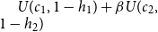 $U(c_{1},1-h_{1})+\beta U(c_{2}, 1-h_{2})$
. Human capital at age 2 is
 $s_2(h_1)$
in the HCA model, a concave increasing function of young labor supply, and an exogenous constant
 $\bar {s}_2$
in the non-HCA model. Budget constraints are:
 \begin{equation} \begin{split} (1+\tau _c)c_{1}+a_{1}&=(1-\tau _h)wh_{1},\\[3pt] (1+\tau _c)c_{2}&=(1+r(1-\tau _k))a_{1}+(1-\tau _h)ws_2(h_1)h_{2}, \end{split} \end{equation}
where
 $\tau _c$
is the consumption tax rate,
 $\tau _h$
is a flat labor income tax rate, and
 $\tau _k$
is the capital income tax rate. The first-order conditions are:
 \begin{equation} \begin{aligned} -\dfrac {U_{h1}}{U_{c1}} &= \dfrac {(1-\tau _h)w}{1+\tau _c}+\underbrace {\dfrac {(1-\tau _h)ws'(h_1)h_{2}}{(1+\tau _c)(1+r(1-\tau _k))}}_{\text{human capital return (HCA only)}},\\[6pt] -\dfrac {U_{h2}}{U_{c2}} &= \dfrac {(1-\tau _h)ws_2(h_1)}{1+\tau _c},\\[6pt] \dfrac {U_{c1}}{U_{c2}} &= \beta (1+r(1-\tau _k)). \end{aligned} \end{equation}
In the non-HCA model the term
 $s'(h_1)=0$
so the first condition reduces to
 $-U_{h1}/U_{c1}=(1-\tau _h)w/(1+\tau _c)$
. The additional term in the HCA model represents the human capital return to young labor: by supplying more hours in period 1, the household raises
 $s_2(h_1)$
, increasing old-age wages. Both
 $\tau _h$
and
 $\tau _c$
enter the two terms symmetrically (
 $\tau _h$
through
 $(1-\tau _h)$
in the numerator,
 $\tau _c$
through
 $(1+\tau _c)$
in the denominator), so neither tax distorts the ratio between the direct wage and human capital incentives. The key mechanism is instead a general equilibrium feedback absent in the non-HCA model: any policy-induced change in
 $h_1$
propagates through
 $s_2(h_1)$
to old-age productivity, wages, savings, and
 $h_2$
. In a revenue-neutral reform that raises
 $\tau _c$
and reduces
 $\tau _h$
, both models experience changes in the labor supply margin, but the HCA model amplifies the aggregate response through this human capital feedback. This is the mechanism behind the steeper aggregate responses (in capital, labor, and output) observed in the HCA model at higher consumption tax rates.
Appendix C. Tables
Progressive consumption tax reform

Table C1. Long description
A table comparing economic indicators under different tax scenarios. The table has 23 rows and 7 columns. Column headers are Baseline, 3 percent comma 5 percent, percent change, 3 percent comma 10 percent, percent change, 3 percent comma 15 percent, and percent change. Row labels include Aggregate, Y, K, N, Avg hours, w, r, beq, CEV, Gini, Consumption, Wealth, Average tax rate, Labor, Capital, Ratio, Marginal tax rate, Labor, Capital, and Ratio. Row 1: Aggregate, Y, 1.17, 1.16, -0.8, 1.16, -0.6, 1.16, -0.5. Row 2: Aggregate, K, 3.14, 3.05, -2.9, 3.10, -1.3, 3.13, -0.4. Row 3: Aggregate, N, 0.67, 0.67, +0.4, 0.67, -0.2, 0.67, -0.5. Row 4: Avg hours, 0.30, 0.30, -0.2, 0.30, -0.9, 0.30, -1.1. Row 5: w, 0.91, 0.91, -0.7, 0.91, -0.7, 0.91, -0.4. Row 6: r, 0.051, 0.054, +5.7, 0.052, +2.1, 0.051, -0.2. Row 7: beq, 0.037, 0.036, -3.9, 0.036, -3.2, 0.037, -2.1. Row 8: CEV, -, -1.14 percent, -, 0.57 percent, -, 2.41 percent. Row 9: Gini, Consumption, 0.31, 0.31, -0.9, 0.30, -2.8, 0.29, -5.2. Row 10: Gini, Wealth, 0.69, 0.68, -0.4, 0.68, -0.2, 0.68, -0.3. Row 11: Average tax rate, Labor, 0.1245, 0.1251, -, 0.1255, -, 0.1258, -. Row 12: Average tax rate, Capital, 0.0861, 0.0865, -, 0.0863, -, 0.0860, -. Row 13: Average tax rate, Ratio, 1.4450, 1.4461, -, 1.4543, -, 1.4632, -. Row 14: Marginal tax rate, Labor, 0.1709, 0.1715, -, 0.1718, -, 0.1721, -. Row 15: Marginal tax rate, Capital, 0.1346, 0.1349, -, 0.1347, -, 0.1344, -. Row 16: Marginal tax rate, Ratio, 1.2697, 1.2709, -, 1.2756, -, 1.2806, -.
Progressive consumption tax reform (cont.)

Table C2. Long description
A table comparing economic indicators under different tax reform scenarios. The table has 18 rows and 10 columns. Column headers are HCA Baseline, 4%, 5%, % change, 4%, 10%, % change, 4%, 15%, % change. Row labels include Aggregate, Avg. hours, Gini Consumption, Wealth, Average tax rate Labor, Average tax rate Capital, Average tax rate Ratio, Marginal tax rate Labor, Marginal tax rate Capital, Marginal tax rate Ratio. Row 1: Aggregate, 1.17, 1.16, 0.5, 1.17, 0.4, 1.16, 0.3. Row 2: K, 3.14, 3.10, 1.6, 3.14, 0.1, 3.17, 0.8. Row 3: N, 0.67, 0.67, 0.1, 0.67, 0.5, 0.67, 0.9. Row 4: Avg. hours, 0.30, 0.30, 0.3, 0.30, 1.0, 0.30, 1.2. Row 5: w, 0.91, 0.91, 0.4, 0.91, 0.4, 0.91, 0.3. Row 6: r, 0.051, 0.052, 2.9, 0.050, 0.7, 0.049, 2.9. Row 7: beq, 0.037, 0.037, 2.2, 0.037, 2.0, 0.037, 0.4. Row 8: CEV, 0.72%, 1.04%, 2.85%. Row 9: Gini Consumption, 0.31, 0.31, 0.3, 0.30, 2.4, 0.29, 4.5. Row 10: Wealth, 0.69, 0.68, 0.1, 0.69, 0.1, 0.69, 0.1. Row 11: Average tax rate Labor, 0.1245, 0.1249, 0.1252, 0.1255. Row 12: Average tax rate Capital, 0.0861, 0.0864, 0.0861, 0.0858. Row 13: Average tax rate Ratio, 1.4450, 1.4454, 1.4542, 1.4618. Row 14: Marginal tax rate Labor, 0.1709, 0.1713, 0.1716, 0.1718. Row 15: Marginal tax rate Capital, 0.1346, 0.1348, 0.1345, 0.1343. Row 16: Marginal tax rate Ratio, 1.2697, 1.2703, 1.2752, 1.2795.
Progressive consumption tax reform (cont.)

Table C3. Long description
A table comparing various economic metrics under different tax reform scenarios. The table has 25 rows and 9 columns. Column headers are HCA, Baseline, 5 percent, 5 percent, percent change, 5 percent, 10 percent, percent change, 5 percent, 15 percent, and percent change. Row labels include Aggregate, Avg hours, Gini, Consumption, Wealth, Average tax rate, and Marginal tax rate. Row 1: Aggregate, Y, 1.17, 1.17, -0.2, 1.17, -0.2, 1.17, -0.1. Row 2: Aggregate, K, 3.14, 3.13, -0.3, 3.17, +1.0, 3.21, +2.0. Row 3: Aggregate, N, 0.67, 0.67, -0.1, 0.67, -0.8, 0.66, -1.3. Row 4: Avg hours, 0.30, 0.30, -0.5, 0.30, -1.0, 0.30, -1.5. Row 5: Aggregate, w, 0.91, 0.91, -0.3, 0.91, -0.2, 0.91, -0.1. Row 6: Aggregate, r, 0.051, 0.051, +0.4, 0.049, -2.9, 0.048, -5.4. Row 7: Aggregate, beq, 0.037, 0.037, -0.2, 0.038, +0.1, 0.038, +0.7. Row 8: Aggregate, CEV, -, -0.37 percent, -, 1.64 percent, -, 3.31 percent. Row 9: Gini, Consumption, 0.31, 0.31, +0.3, 0.31, -2.0, 0.31, -4.2. Row 10: Gini, Wealth, 0.69, 0.68, -0.1, 0.69, +0.4, 0.69, +0.5. Row 11: Average tax rate, Labor, 0.1245, 0.1246, -, 0.1248, -, 0.1252, -. Row 12: Average tax rate, Capital, 0.0861, 0.0862, -, 0.0859, -, 0.0858, -. Row 13: Average tax rate, Ratio, 1.4450, 1.4457, -, 1.4525, -, 1.4598, -. Row 14: Marginal tax rate, Labor, 0.1709, 0.1710, -, 0.1712, -, 0.1716, -. Row 15: Marginal tax rate, Capital, 0.1346, 0.1346, -, 0.1344, -, 0.1342, -. Row 16: Marginal tax rate, Ratio, 1.2697, 1.2702, -, 1.2740, -, 1.2783, -.
Progressive consumption tax reform (cont.)

Table C4. Long description
A table comparing economic metrics under different tax reform scenarios. The table has 12 rows and 9 columns. Column headers are Baseline, 3 percent, 5 percent, percent change, 3 percent, 10 percent, percent change, 3 percent, 15 percent, and percent change. Row labels include Aggregate, Y, K, N, Avg. hours, w, r, beq, CEV, Gini, Consumption, Wealth, Average tax rate, Labor, Capital, Ratio, Marginal tax rate, Labor, Capital, and Ratio. Row 1: Aggregate, Row 2: Y, 1.18, 1.18, 1.18, -0.7, 1.18, -0.3, 1.19, +0.02, Row 3: K, 3.17, 3.08, 3.15, -2.7, -0.3, 3.21, +1.5, Row 4: N, 0.68, 0.69, 0.68, +0.4, -0.3, 0.68, -0.8, Row 5: Avg. hours, 0.33, 0.33, 0.33, -0.4, -1.2, 0.33, -1.9, Row 6: w, 0.93, 0.92, 0.92, -0.7, -0.3, 0.93, +0.01, Row 7: r, 0.052, 0.054, 0.052, +5.3, +0.1, 0.050, -3.8, Row 8: beq, 0.040, 0.039, 0.040, -2.9, -1.5, 0.040, -0.2, Row 9: CEV, -, -0.76 percent, -, 1.84 percent, -, 4.19 percent, -, Row 10: Gini, Row 11: Consumption, 0.34, 0.33, 0.33, -0.9, -3.4, 0.32, -6.1, Row 12: Wealth, 0.76, 0.76, 0.76, -0.04, +0.2, 0.76, +0.1, Row 13: Average tax rate, Row 14: Labor, 0.1259, 0.1263, 0.1265, -, -, 0.1268, -, Row 15: Capital, 0.0976, 0.0983, 0.0978, -, -, 0.0973, -, Row 16: Ratio, 1.2897, 1.2856, 1.2941, -, -, 1.3036, -, Row 17: Marginal tax rate, Row 18: Labor, 0.1723, 0.1726, 0.1728, -, -, 0.1731, -, Row 19: Capital, 0.1455, 0.1461, 0.1456, -, -, 0.1451, -, Row 20: Ratio, 1.1841, 1.1819, 1.1871, -, -, 1.1927, -
Progressive consumption tax reform (cont.)

Table C5. Long description
A table comparing economic indicators under different tax reform scenarios. The table has 18 rows and 10 columns. Column headers are Baseline, 4%, 5%, % change, 4%, 10%, % change, 4%, 15%, % change. Row labels include Aggregate, Y, K, N, Avg. hours, w, r, beq, CEV, Gini, Consumption, Wealth, Average tax rate, Labor, Capital, Ratio, Marginal tax rate, Labor, Capital, Ratio. Row 1: Aggregate, 1.18, 1.18, 0.5, 1.19, 0.05, 1.19, +0.2. Row 2: Y, 1.18, 1.18, 0.5, 1.19, 0.05, 1.19, +0.2. Row 3: K, 3.17, 3.12, 2.7, 3.19, 0.3, 3.25, +2.7. Row 4: N, 0.68, 0.68, +0.1, 0.68, 0.6, 0.68, 1.1. Row 5: Avg. hours, 0.33, 0.33, 0.6, 0.33, 1.4, 0.33, 2.2. Row 6: w, 0.93, 0.92, 0.5, 0.93, 0.05, 0.93, +0.2. Row 7: r, 0.052, 0.053, +2.8, 0.050, 2.4, 0.047, 6.2. Row 8: beq, 0.040, 0.040, 1.7, 0.040, 0.3, 0.041, +0.9. Row 9: CEV, 0.43%, 2.31%, 4.64%. Row 10: Gini, Consumption, 0.34, 0.34, 0.3, 0.33, 2.9, 0.32, 5.5. Row 11: Wealth, 0.76, 0.76, 0.1, 0.76, +0.1, 0.76, +0.1. Row 12: Average tax rate, Labor, 0.1259, 0.1262, 0.1264, 0.1267. Row 13: Capital, 0.0976, 0.0979, 0.0974, 0.0970. Row 14: Ratio, 1.2897, 1.2890, 1.2980, 1.3064. Row 15: Marginal tax rate, Labor, 0.1723, 0.1725, 0.1727, 0.1730. Row 16: Capital, 0.1455, 0.1457, 0.1452, 0.1448. Row 17: Ratio, 1.1841, 1.1839, 1.1893, 1.1943.
Progressive consumption tax reform (cont.)

Table C6. Long description
A table comparing economic indicators under different tax reform scenarios. The table has 12 rows and 9 columns. Column headers are Baseline, 5 percent comma 5 percent, percent change, 5 percent comma 10 percent, percent change, 5 percent comma 15 percent, and percent change. Row labels include Aggregate, Y, K, N, Avg. hours, w, r, beq, CEV, Gini, Consumption, Wealth, Average tax rate, Labor, Capital, Ratio, and Marginal tax rate. Row 1: Aggregate, Y, 1.18, 1.18, -0.2, 1.19, +0.1, 1.19, +0.5. Row 2: K, 3.17, 3.15, -0.4, 3.23, +2.0, 3.29, +3.9. Row 3: N, 0.68, 0.68, -0.1, 0.68, -0.9, 0.67, -1.4. Row 4: Avg. hours, 0.33, 0.33, -0.8, 0.33, -1.7, 0.33, -2.5. Row 5: w, 0.93, 0.92, -0.2, 0.93, +0.1, 0.93, +0.5. Row 6: r, 0.052, 0.052, +0.5, 0.049, -4.7, 0.047, -8.6. Row 7: beq, 0.040, 0.040, -0.4, 0.041, +0.7, 0.041, +1.9. Row 8: CEV, -, -0.07 percent, -, 2.68 percent, -, 5.12 percent, -. Row 9: Gini, Consumption, 0.34, 0.34, +0.3, 0.33, -2.4, 0.32, -4.9. Row 10: Wealth, 0.76, 0.76, -0.05, 0.76, +0.1, 0.76, +0.2. Row 11: Average tax rate, Labor, 0.1259, 0.1261, -, 0.1263, -, 0.1266, -. Row 12: Capital, 0.0976, 0.0977, -, 0.0970, -, 0.0966, -. Row 13: Ratio, 1.2897, 1.2916, -, 1.3015, -, 1.3097, -. Row 14: Marginal tax rate, Labor, 0.1723, 0.1724, -, 0.1726, -, 0.1729, -. Row 15: Capital, 0.1455, 0.1455, -, 0.1449, -, 0.1445, -. Row 16: Ratio, 1.1841, 1.1853, -, 1.1912, -, 1.1961, -.


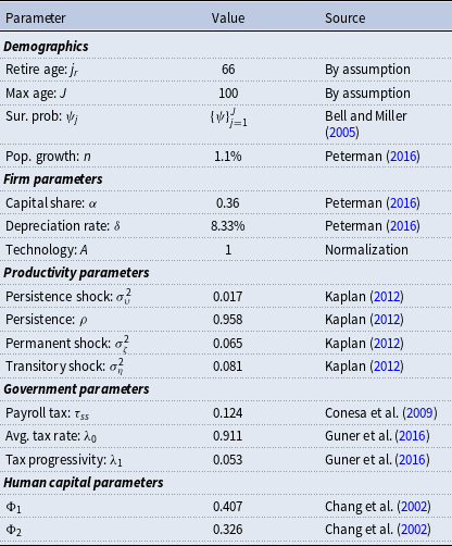
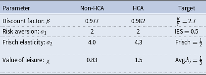
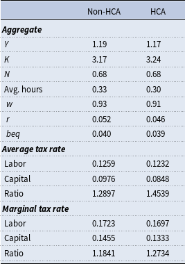
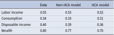


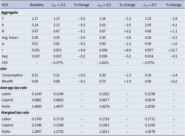
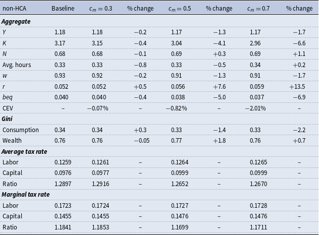
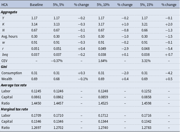
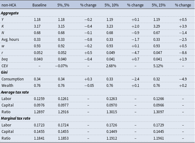
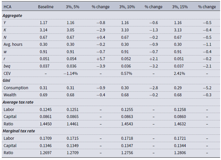
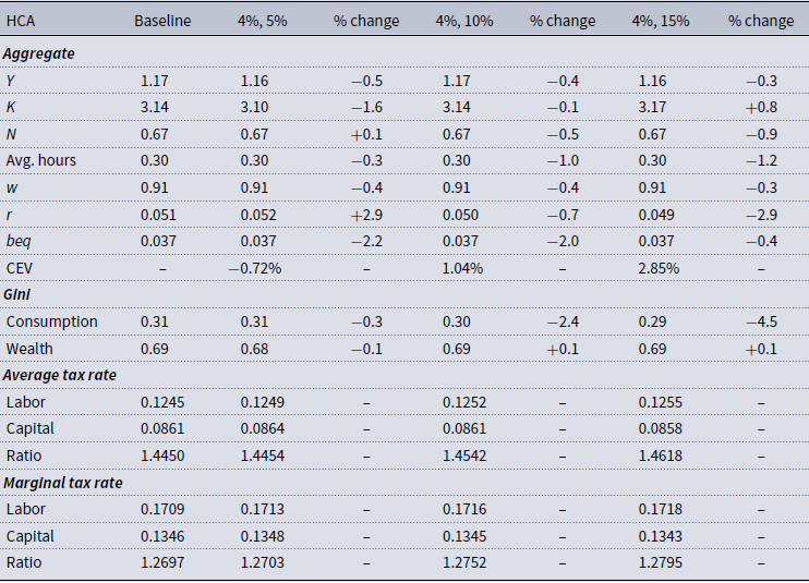
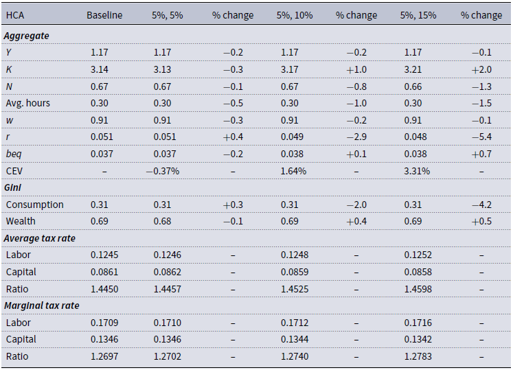
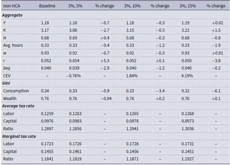
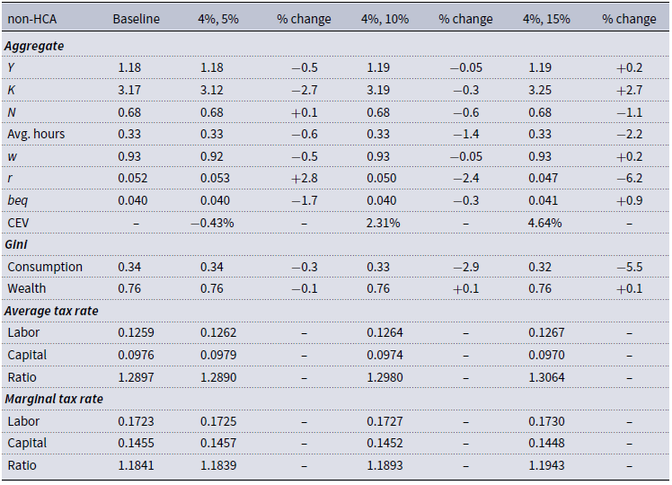
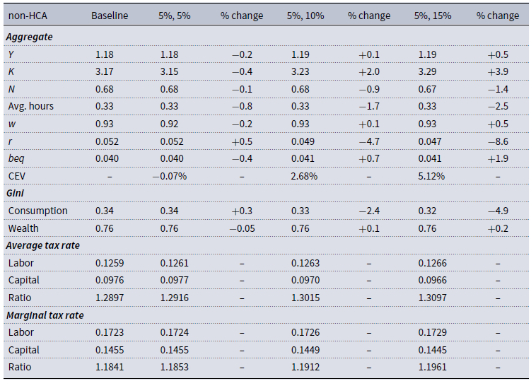

 Open access

