2 Background

The development of artist robots has received great interest since 1990. AARON, one of the oldest continuously developed programs in computing history (beginning in the mid-70’s), attempted to create paintings that produced human-like artworks (Cohen, Reference Cohen1994). Gommel et al . (2004) implemented an industrial robotic arm, KUKA, to draw in Cartesian space. Srikaew et al. (1998) created a dual-armed humanoid robot, ISAC, that used the control of the end-effector with force sensors in the process of drawing. Ruchanurucks and Kudoh also implemented a multi-fingered robot called Dot-chan which was equipped with position- and force-sensing (Ruchanurucks et al., Reference Ruchanurucks, Kudoh, Ogawara, Shiratori and Ikeuchi2007; Kudoh et al., Reference Kudoh, Ogawara, Ruchanurucks and Ikeuchi2009) to produce color brush drawing. Katsura and his group have developed a calligraphy robot based on their Motion Copy System (Tsunashima & Katsura, Reference Tsunashima and Katsura2010) which learn the input calligraphy motion (e.g. position and pressure) to reproduce the brush strokes (Kennedy & Osuga, Reference Kennedy and Osuga2012). Tresset and Fol Leymarie created AIKON/Skediomata a 3-d.f. low-cost robotic platform dedicated to drawing sketches (Tresset & Leymarie, Reference Tresset and Leymarie2005, Reference Tresset and Leymarie2006; Tresset et al., Reference Khaorapapong2011). Calinon et al . from École Polytechnique Fédérale de Lausanne (EPFL) used the small humanoid robot HOAP2 for their human portrait drawing task (Calinon et al., Reference Calinon, Epiney and Billard2005). Pica was introduced by Lin et al . for fast human portrait drawing but its drawing results were very simple and lacked contours (Lin et al., Reference Lin, Chuang and Mac2009). Another interesting approach was Drawbot, a wheeled-robot with a pen-holder mounted on an arm that allowed the pen to be lifted off the drawing surface (Brown et al., Reference Brown, Bigge, Bird, Husbands, Perris and Stokes2005). A similar approach is used in a polargraph art robot, Makelangelo developed by a robotic company called Marginally Clever (2013). It used a wall-drawing approach which draws on a piece of paper on the wall with a pen that adjusts its x-y position based on two strings controlled by two stepper motors. Lu et al . (2009) developed a robotic manipulator called IRAS based on visual feedback that determines stroke positions and applies local gradient interpolation to guide stroke orientation in its pen-and-ink artwork. However, this was only in a fixed plotter-like setting. In order to improve the drawing accuracy, some researches try to implement machine learning approaches such as deep neural network (Sasaki et al., Reference Sasaki, Noda and Ogata2016; Singh et al., Reference Singh, Baranwal and Nandi2017; Atoofi, Reference Atoofi, Hamker and Nassour2018). An in-depth review of these works shows that none of them used visual servoing in humanoid robots as feedback for drawing observation, and none provides drawing correction during the drawing process. This is an important ability in pen and ink sketching. In this paper, we implemented a closed-loop image-based visual servoing (IBVS) control techniques to address the drawing deviation problem of our robot.

Creating a artist humanoid robot with high-performance industrial robots (i.e. accurate and fast) usually involves a high hardware cost. It is a much more significant challenge to develop an efficient robotic system if the cost is also an important factor. Reducing the cost of the system requires optimization of all aspects to retain its flexibility, reliability and performance. During the design and development of our humanoid robot, namely, Betty, we only used affordable hardware and open-source software to address both cost (approximately USD 3000) and performance issues (Baltes et al., Reference Baltes, Cheng, Lau and Anderson2011). The upper body of Betty consists of a 12-revolute joint system with 12 degrees of freedom (d.f.). Its head has 4 d.f. which are pan, tilt, swing and one d.f. for the mouth. Each of its arms provides 4 d.f., shoulders allow lateral and frontal motions and elbow gives lateral motion and a wrist motion. These joints are constructed by four Dynamixel RX-64 servos in the head and four Dynamixel RX-64 servos for each of its arms as shown in Section 4. The visual feedback control is driven by an open-source computer vision library (OpenCV) which has various image processing techniques. These techniques compute a line-art output vector that can be mapped to the kinematics of Betty’s arm. This research aims to develop a robust visual servoing sketch drawing system that enables Betty to autonomously draw the sketches by exploring various research areas.

Due to the hardware performance limitations, it is difficult to achieve high mechanical accuracy. One of the main motivations of our work is to develop a closed-loop approach which is significantly superior to open-loop control to overcome the lack of accuracy in our humanoid robot. This non-feedback or ‘blinded’ open-loop approach might not be adequate for a sophisticated implementation of a drawing robot because it does not provide sufficient feedback during the drawing process. When using an open-loop control in a robotic system, there is no online interaction between the robot and the environment where no data is collected from the robot’s sensors during task execution which can be seen in Franklin et al. (Reference Franklin, Powell and Emami-Naeini2001), Instruments (Reference Instruments2011). At first, it extracts the information from an input image. From this, it generates a robot pose and motion sequence. This allows the control of a robot and image processing to be viewed as two independent tasks (Kragic & Christensen, Reference Kragic and Christensen2002). One of the main disadvantages of this approach is that the robot will not be able to correct its state if there are any changes in its environment during the process (Instruments, Reference Instruments2011). For instance, in our earlier implementation of our sketch drawing humanoid robot, the portrait of a person is recognized and extracted, then its pixels position is computed relative to the camera (robot) coordinate system. This Cartesian space information is used to move Betty’s arm to the desired position relative to the drawing pad. With the eye-to-hand camera and inverse kinematic model, the position of the pen is computed based on the visual information extracted from the camera frame. It then maps the pixels of the image to Betty’s inverse kinematic model. Next, Betty executes the drawing task by performing open-loop movements which assumes that the environment remains static after the drawing has started (Baltes et al., Reference Baltes, Cheng, Lau and Anderson2011). However, without the real-time feedback of what has been drawn by Betty, it is impossible to make corrections to ensure the desired output sketch which is obtained at the end. Hence, we need a closed-loop control system to overcome this problem.

3 Image-based visual servoing

Visual servoing is a common closed-loop visual feedback control approach for object manipulation in robotic research, for example (Bourquardez et al., Reference Bourquardez, Mahony, Hamel and Chaumette2006; Vahrenkamp et al., Reference Vahrenkamp, Wieland, Azad, Gonzalez, Asfour and Dillmann2008, Reference Vahrenkamp, Boge, Welke, Asfour, Walter and Dillmann2009; Siradjuddin et al., Reference Siradjuddin, Behera, McGinnity and Coleman2010; Chu et al., Reference Chu, Mills and Cleghorn2011) and industry, for example (Hodges & Hall, Reference Hodges and Hall1996; Nomura & Naito, Reference Nomura and Naito2000). In contrast to open-loop control, a closed-loop control system uses vision as the feedback sensor to continuously track the environment, which provides estimation and updates for robot control and positioning. Therefore, the control sequence is generated based on a consistent visual feedback of the error between its current and desired poses of the end-effector. The terminology of visual servoing was introduced in 1979 by Hill and Park (1979) prior to the general term ‘visual feedback’ (Hutchinson et al., Reference Hutchinson, Hager and Corke1996). Generally, visual servoing techniques are classified into three types: IBVS, position-based visual servoing (PBVS) and advanced visual servoing (Chaumette & Hutchinson, Reference Chaumette and Hutchinson2006, Reference Chaumette and Hutchinson2007). The general idea of a visual servoing system is to estimate the differential changes between robot joint space and the image space with a coupled robot-image Jacobian (Kragic & Christensen, Reference Kragic and Christensen2002).

PBVS processes the error signal from the image features in order to compute the control sequence of the robot based on the relative 3D pose between the camera and the end-effector (Wilson et al., Reference Wilson, Williams Hulls and Bell1996; De Luca et al., Reference De Luca, Oriolo and Giordano2007). PBVS solves the 3D localization problem where 3D information of the scene, including a geometric model of the target, and the parameters of the particular camera model (camera calibration) is known. PBVS is considered to be a 3D vision sensor. Usually, there are two tasks in a PBVS system. First, as mentioned, it requires a model between camera and end-effector to estimate the pose of the target. Second, it has to estimate the desired velocity screw of the robot, which requires precise camera-robot calibration to achieve accurate positioning (Kragic & Christensen, Reference Kragic and Christensen2002).

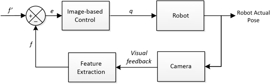
Image-based visual servo systems (IBVSs) were introduced by Weiss and Sanderson (Weiss et al., Reference Weiss, Sanderson and Neuman1985; Weiss & Sanderson, Reference Weiss and Sanderson1987) to compute the pose of the robot by processing the error signal from the image features parameters, for example, lines and image areas directly as its feedback control signals (De Luca et al., Reference De Luca, Oriolo and Giordano2007). IBVS involves the computation of the image Jacobian or the interaction matrix (Hutchinson et al., Reference Hutchinson, Hager and Corke1996; Kragic & Christensen, Reference Kragic and Christensen2002). In contrast to PBVS, IBVS is considered as a 2D vision sensor. IBVS eliminates PBVS’s requirement of perfect knowledge of the camera calibration matrix and its complex interpretation of image features to derive 3D world-space coordinates. Figure 1 shows the general design of an IBVS system.

Figure 1.

Block diagram of IBVS. f is the actual location of feature and f ^′ is its desired location. The positioning task is described as location error, $e=f-f'$ and q represents the coordinate of the end-effector.

In our sketch drawing humanoid robot research, a 2D image (from the drawing pad) is used directly to estimate the desired pose of Betty’s arm. This is a typical task of IBVS, where the image distance error (drawing variation) between the current and desired image features in the output image plane is tracked. We therefore proposed to use IBVS to address this problem in our work. Generally, IBVS can be divided into two separate systems. First, a dynamic look-and-move system. This system performs the control of the robot in two stages: the vision system provides input to robot controller that then uses joint position feedback to control the end-effector. As pointed out by Hutchinson et al ., nearly all of the reported systems adopt this approach (1996). Second, direct visual servo systems. Here, the visual controller directly computes the input to the robot joints and robot controller is eliminated (no position feedback) (Kragic & Christensen, Reference Kragic and Christensen2002). As discussed by Chaumette and Hutchinson, there is no strategy that provides perfect properties based on their stability issues (Chaumette & Hutchinson, Reference Chaumette and Hutchinson2006). However, the coarse estimations in IBVS will only imply perturbations in the trajectory performed by the robot to reach its desired pose (longer convergence time) and will have no effect on the accuracy of the pose reached. On the other hand, IBVS has several advantages over PBVS. In IBVS, a 3-D environment model is not required. Its target always stays in the field of view of the camera, and its performance is robust with respect to camera calibration errors and noise when a monocular camera is used (Bourquardez et al., Reference Bourquardez, Mahony, Hamel and Chaumette2006; Chaumette & Hutchinson, Reference Chaumette and Hutchinson2006; De Luca et al., Reference De Luca, Oriolo and Giordano2007). Therefore, we use this image-based eye-to-hand visual servoing to control the relative pose between the drawing tool and the drawing pad with a camera mounted on Betty’s head.

For the drawing task, a camera (right eye) is used as a global vision sensor (eye-to-hand configuration). It retrieves and tracks the position of the features (lines and shading) in the image relative to the Betty’s inverse kinematic frame. Compared to PBVS, IBVS’s great robustness with respect to calibration error can thus be expected. As discussed earlier, a visual servoing approach is classified based on the type of feedback it perceived. In our implementation, we extracted the line segments of the drawing pad’s pen-and-ink sketch. Based on this information, it guides Betty during the drawing process to correct the drawn errors (e.g. line segments pose: two end-points and completeness). Hence, an IBVS approach is implemented.

IBVS involved manipulation of a set of image features (object) from an acquired image based on their coordinates by computation of the image Jacobian (Kragic & Christensen, Reference Kragic and Christensen2002). In general, the Jacobian matrix (J) is defined as a matrix based on the motion of the image feature. J is used to set the desired pose of manipulator as seen in Equation (1) (Hutchinson et al., Reference Hutchinson, Hager and Corke1996; Kragic & Christensen, Reference Kragic and Christensen2002).

(1) \begin{equation}\label{eqn1}\dot{f}=J\dot{q}\end{equation}

Where $\dot{f}$ represents the motion of the image feature in consecutive images and $\dot{q}$ denotes the six dimension velocities, $[\dot{x},\dot{y},\dot{z},\dot{w_{x}},\dot{w_{y}},\dot{w_{z}}]$ : three translations and three rotations of the feature with respect to the camera frame (Chu et al., Reference Chu, Mills and Cleghorn2011). Based on the unit focal length perspective projection model, the relationship between the robot arm and the image feature is shown as Equation (2) (Hutchinson et al., Reference Hutchinson, Hager and Corke1996; Kragic & Christensen, Reference Kragic and Christensen2002).

(2) \begin{equation}\label{eqn2}\begin{bmatrix}\phantom{\,}\dot{x'}\phantom{\,} \\[15pt]\dot{y'}\end{bmatrix}=\begin{bmatrix}\dfrac{1}{Z} &\quad 0 &\quad -\frac{x}{Z} &\quad xy &\quad (1+x^{2}) &\quad -y \\[7pt]0 &\quad \dfrac{1}{Z} &\quad -\frac{y}{Z} &\quad -(1+y^{2}) &\quad xy &\quad x\end{bmatrix}\end{equation}

During the drawing task, the pen’s tip is orthogonal to the surface of the drawing pad. Hence, no orientation adjustment is required during the servoing. The image features only need to be translated to the desired pose with the three translation $[\dot{x},\dot{y},\dot{z}]$ workspace. Therefore, the Jacobian can be simplified as Equation (3).

(3) \begin{equation}\label{eqn3}J =\left[\begin{array}{c@{\quad}c@{\quad}c}\frac{1}{Z} & 0 & -\frac{x}{Z} \\[8pt]0 & \frac{1}{Z} & -\frac{y}{Z}\end{array}\right]\end{equation}

IBVS expresses the control error function directly in 2D image space (Kragic & Christensen, Reference Kragic and Christensen2002). The aim of all vision-based control schemes is to minimize the error e(t), which is typically defined as $e(t) = f - f'$ where its block diagram is shown in Figure 1. f is a vector of n visual features based on image measurements (e.g. the image coordinates of interest points, or the parameters of a set of image segments) and a set of parameters that represent partial knowledge about the system (e.g. camera intrinsic parameters or three-dimensional object models) (Siradjuddin et al., Reference Siradjuddin, Behera, McGinnity and Coleman2010). The vector f ^′ is the desired values of these features. In the drawing tasks, the simplest model for the controller is its drawing deviation. And, there must be a relationship between the time variation of each variable.

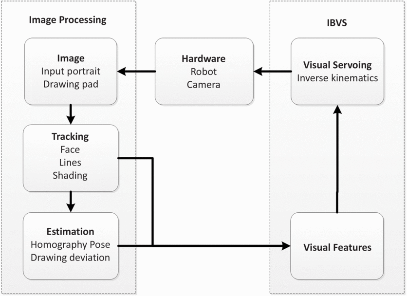
Based on Kragic et al .’s (Kragic & Christensen, Reference Kragic and Christensen2002) and Chu et al .’s research (2011), the most common proportional control approach is applied to generate the control signal for the robot. $J^{-1}$ is the pseudoinverse of the image Jacobian and $K_{p}$ is the proportional gain. The visual servoing scheme continues until the evaluated error is less than the given threshold pixels limit on the image. Figure 2 illustrates the proposed framework of the visual processing pipeline for the IBVS system.

(4) \begin{eqnarray}\label{eqn4}\dot{q}=\begin{bmatrix}\phantom{\,}\dot{x}\phantom{\,} \\[3pt]\dot{y} \\[3pt]\dot{z}\end{bmatrix}=K_{p}J^{-1} \cdot e(t)\end{eqnarray}

Figure 2.

General framework of IBVS for drawing task.

Let us assume the camera position is static and the height of the drawing pad is known. A number of feature lines are tracked and used to generate a vector of current measurements, $f_{1}$ and $f_{2}$ . The vector of desired reference measurements is denoted $f'_{1}$ and $f'_{2}$ . The error function for the drawing deviation is defined as a function of the distance between these measurements, $e = f - f'$ . This error function is then updated in each frame and used together with the inverse kinematics to estimate the control input to Betty.

3.1 Drawing pad detection and sketch extraction

Drawing pad location is a crucial information in the IBVS implementation. Based on this information, it constructs the image plane on a Cartesian space to extract content on the drawing pad.

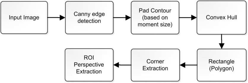
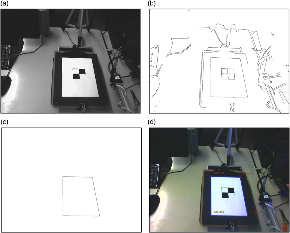
Figure 3 shows the overall process to detect the drawing pad location and to extract its content within the drawing area. First, we applied the Canny edge detector to the input image to obtain the line image as seen in Figure 4(b). With the wide range of edges in the image, drawing pad contour is extracted based on its moments size by using the moments function in OpenCV. It allows computation of all moments as seen in Equation (5)  (Team, Reference Team2013b).

(5) \begin{equation}\label{eqn5}m_{ij}=\sum_{x,y} (array(x,y) \cdot x^{\,j} \cdot y^{i} )\end{equation}

Figure 3.

Flowchart for drawing pad detection.

Figure 4.

Image pipeline for drawing pad detection. (a) Input image; (b) Canny line detection output; (c) pad contour of drawing area is extracted; (d) four corners are estimated based on rectangular convex hull.

We used a rectangular convex hull algorithm as the minimum bounding box of the rectangle drawing area to compute its four corners’ coordinates in Figure 4(d). Last, based on the detected corners vertices, a perspective transformation is performed to map the deformed drawing pad (region of interest (ROI)) to its destination image. The mapping is done by getPerspectiveTransform and warpPerspective in OpenCV library (Team, Reference Team2013a). Equation 6  (Team, Reference Team2013a) shows the calculation of the 3 $\times$ 3 perspective transform matrix from four pairs of the corresponding points $i=0,1,2,3$ . The destination image vertices are represented as $dst(i) = (x'_{i},y'_{i})$ , and the source image vertices are referred as $src(i) = (x_{i},y_{i})$ .

(6) \begin{eqnarray}\label{eqn6}\begin{bmatrix}t_{i}x'_{i} \\[3pt]t_{i}y'_{i} \\[3pt]t_{i}\end{bmatrix}& = &map\_matrix\cdot\begin{bmatrix}\phantom{\,}x_{i}\phantom{\,} \\[3pt]y_{i} \\[3pt]1\end{bmatrix}\end{eqnarray}

Then, we used the warpPerspective function to perform a perspective transformation of a source image to a destination image using the specified 3 $\times$ 3 matrix, M to correct distortion caused by viewing angle of Betty right eye. Mapping of the drawing pad dimension is described in Equation (7) (Team, Reference Team2013a). Figure4 shows an example of extracted drawing pad area.

(7) \begin{equation}\label{eqn7}dst(x,y)=src\left(\dfrac{M_{11}x+M_{12}y+M_{13}}{M_{31}x+M_{32}y+M_{33}},\dfrac{M_{21}x+M_{22}y+M_{23}}{M_{31}x+M_{32}y+M_{33}}\right)\end{equation}

3.2 Sketch lines matching

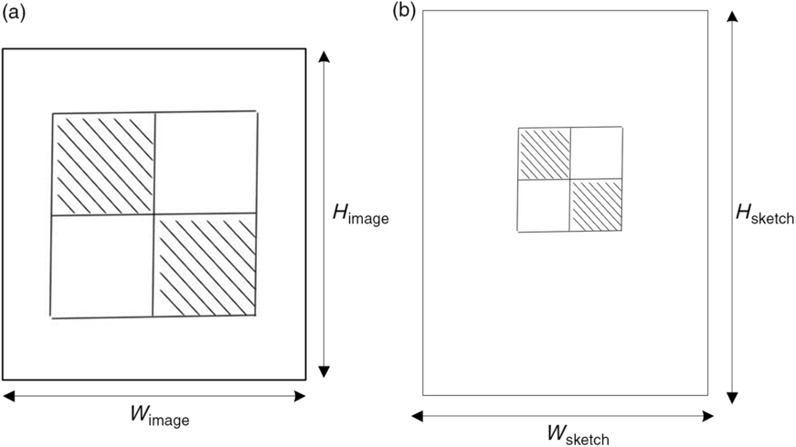
Sketch line matching is the process to match line segments based on geometrically possible pairs of generated sketch and actual drawn lines segments to compensate for drawing errors for the IBVS approach. This technique is adapted and extended from the edge drawing lines (EDLines) algorithm (Akinlar & Topal, Reference Akinlar and Topal2011a, Reference Akinlar and Topalb). First, the ROI of an input image is defined and used the standard EDLines algorithm to detect line segments. These line segments are sorted by their y-coordinate. Next, line segments that lay near the edges of the sketch and short insignificant lines (based on the given threshold, e.g. line segments with fewer than 10 pixels) are removed from the line vectors. The final step is to merge all near-collinear line segments to minimize the number of significant line segments. Then, the geometry of the drawing pad is mapped to the generated sketch dimension in 2D space (x- and y-coordinates) as shown in Figure 5 with directional scaling from Figure 5(a) and (b). Its projective transformation matrix is shown in Equation 8, where $s_{x} = W_{\rm sketch}/W_{\rm image}$ and $s_{y} = H_{\rm sketch}/H_{\rm image}$ .

Figure 5.

Image mapping from input image to sketch for drawing pad. (a) Input image and (b) mapped sketch based on drawing pad dimension.

(8) \begin{eqnarray}\label{eqn8}\begin{bmatrix}x_{\rm image} \\[3pt]y_{\rm image} \\[3pt]1\end{bmatrix}=\begin{bmatrix}s_{x} & \quad 0 & \quad 0\\[3pt]0 & \quad s_{y} & \quad 0 \\[3pt]0 & \quad 0 & \quad 1\end{bmatrix}\cdot\begin{bmatrix}x_{\rm sketch} \\[3pt]y_{\rm sketch} \\[3pt]1\end{bmatrix}=\begin{bmatrix}s_{x} x_{\rm sketch} \\[3pt]s_{y} y_{\rm sketch} \\[3pt]1\end{bmatrix}\end{eqnarray}

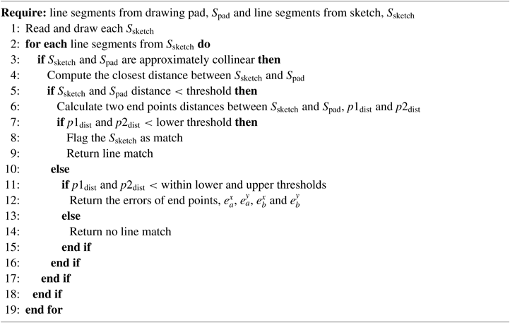
Each of the line segments will be redrawn based on the correction of its position error. Errors of two end points of a line segment convey the errors of angle and length of the matching line segment to its desired baseline. It provides sufficient information to redraw the unmatched line segment. However, if the matching is unsuccessful after several trials, the drawing process will move on to the next line segment to avoid infinite loop of single line segment matching. We use five-trial as the termination condition for each line segment.

Algorithm 1

Match line segments

The error function is defined simply as the difference between the current (or the closest line segment) and the desired line segment feature $e(t) = f - f'$ . Based on their two end points where f is the pose of the current line segment ab and fʹ is its desired pose which is aʹbʹ, hence, the current errors e(t) of endpoints a and b in 2D space could be defined as the Manhanttan distance between them:

(9) \begin{eqnarray}\label{eqn9}e_{a}(t) = dist(a,a') = [e_{a}^{x}, e_{a}^{y}] = [(x_{a}-x'_{a}) , (y_{a}-y'_{a})] \\[5pt]e_{b}(t) = dist(b,b') = [e_{b}^{x}, e_{b}^{y}] = [(x_{b}-x'_{b}) , (y_{b}-y'_{b})] \nonumber\end{eqnarray}

(10) \begin{eqnarray}\label{eqn10}a_{IK}^{x}(t) = a_{IK}^{x}(t-1) + K_{p}*e_{a}^{x}\\[5pt]a_{IK}^{y}(t) = a_{IK}^{y}(t-1) + K_{p}*e_{a}^{y} \nonumber \\[5pt]b_{IK}^{x}(t) = b_{IK}^{x}(t-1) + K_{p}*e_{b}^{x} \nonumber \\[5pt]b_{IK}^{y}(t) = b_{IK}^{y}(t-1) + K_{p}*e_{b}^{y} \nonumber\end{eqnarray}

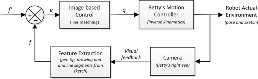
Then, these errors are passed to the inverse kinematics routine to change the joint angles to the desired pose with a P controller. Equation (10) shows the proportional control function where $K_{p}$ is a empirically tuned gain. The third dimension z could only be estimated based on no-touch events. The process of the line segments matching is shown in Algorithm 1. No transfer of errors from one stroke to the next. It avoids false corrections due to shifting of drawing pad during the drawing task. Figure 6 shows the closed-loop control diagram for the IBVS algorithm.

Figure 6.

Closed-loop control diagram for IBVS.

4 Experimental setup and results

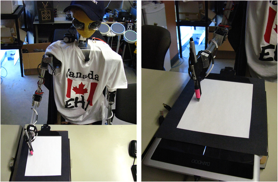
In the experiments, we evaluated the feasibility of our IBVS control based implementation on their drawn outputs. Figure 7 shows the experimental setup of Betty. During the experiments, Betty used its right arm to draw. We used sinusoidal interpolation for its motion trajectory. We placed a Wacom Bamboo tablet (CTH670M) under the paper to measure position and pressure on the drawing pad. The measures of the tablet were only used to establish the reliability of the experiments but did not provide any feedback control to Betty. The drawing area of 217 mm by 137 mm is based on the specification provided by the manufacturer with the accuracy of $\pm$ 0.5 mm.

Figure 7.

Experimental setup using a Wacom Bamboo tablet (CTH640M), Betty, camera and pen.

The efficiency of the IBVS control approach was tested based on two given x- and y- position errors of 10 and 20 mm offset from the correct line segment. Betty repeated 30 times for each stroke type of vertical, horizontal and diagonal lines based on these two offsets for a total of 90 trails in each initial offset error. Only one direction of strokes (downward and left-right) was examined in this experiment because it had no effect on visual information. For these trials, the average errors in the position for each type of stroke were measured. Next, we calculated the absolute differences of the current position of two endpoints, $p_{1}$ and $p_{2}$ ; and the desired position, $p{'}_{1}$ and $p{'}_{2}$ as mapped by the tablet where $e_{pi} = dist(p_{i},p{'}_{i})$ , $i =1,2$ and dist is the Euclidean distance between two end points of $p_{i}$ and $p{'}_{i}$ . We selected the proportional gain, $K_{p} = 0.4$ empirically during the experiment. Figure 8 shows the result if the drawing is moved during the experiment and Figure 9 shows how line segments were perceived from the camera.

Figure 8.

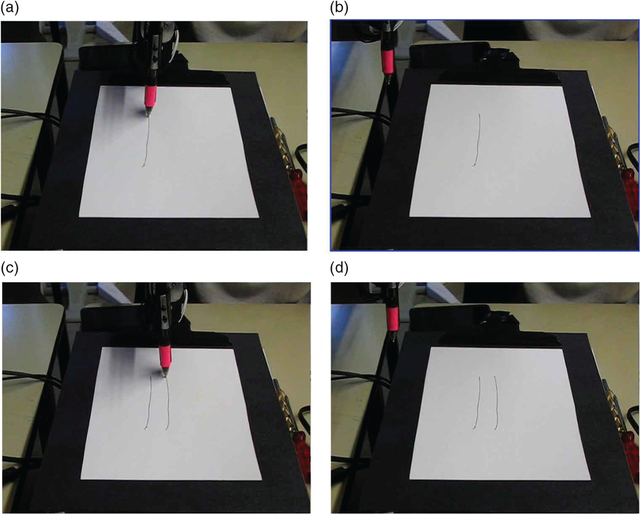
Example of vertical stroke error correction with IBVS control. (a) a faulty line is drawn with the given offset. (b) The hand is moved away from the drawing pad to avoid occlusion. (c and d) A correct line segment was drawn in second trial after error correction based on its line segment’s feature.

Figure 9.

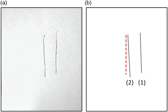
Line segments perceived from the camera. (a) Input ROI image as seen from camera, (b) line segments detected by eEDLines approach (1) is the first stroke, (2) is the corrected stroke and the dotted line is the desired line segment.

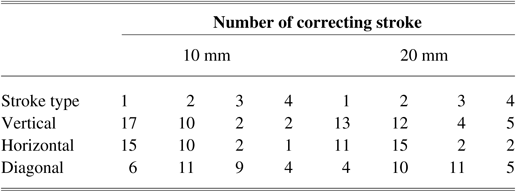
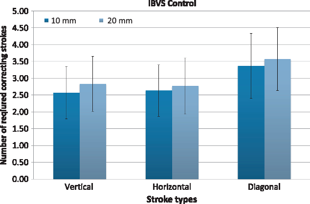
Table 1 shows the number of required correcting strokes to the initial offset errors and how they converged to their desired distance from their baselines (correct line segments). The results clearly show that the 10 mm offset error was successfully corrected within two to three strokes for vertical and horizontal strokes. It reduced the error to approximately 5 mm from the desired baseline. However, diagonal strokes did not show good convergence on average. Based on our observation, it was caused by the sinusoidal drawing motion at the wrist that is likely to create curvy lines. Therefore, we used linear interpolation in this matter but small vibration at the pen’s tip caused by the non-smooth trajectory created jerking lines. This problem introduced significant noise to the existing line segment detection algorithm and affected the results. Similarly to 10 mm offset experiments, 20 mm offset error shows consistent convergence of vertical and horizontal strokes. However, due to the drawing motion trajectory; diagonal strokes remained harder to correct, often requiring 4-stroke and 5-stroke. In this experiment, we labeled five-stroke trails as correction failures. IBVS control approach had the failure rate of 13% and 17% in diagonal strokes compare to lower failure rate of nearly 3% in vertical and horizontal strokes for 10 mm and 20 mm offsets, respectively. Figure 10 shows the averages of trails needed to make the correction of each stroke type in both 10 and 20 mm offset conditions.

Table 1.

Number of correcting strokes required based on the initial errors

Figure 10.

Number of strokes for different stroke types based on IBVS control. Error bars indicate the standard deviation.

5 Conclusion

In this work, we implemented a new approach for the drawing robot to visual servo the sketch drawing task, using an IBVS technique. The results show that this approach has successfully translated the drawing deviation into control actions within the drawing task. In our work, we used a Bamboo tablet and a series of experiments to provide the capability of drawing evaluation. This may lead to a better understanding of the various components, such as the correlation between pressure and drawing (pixels) deviation in different implementations.

As future work, we would like to improve the visual feedback of the drawing task by investigating better line segment detection algorithms. Such as, a line detection algorithm proposed by Liu et al . (Reference Liu, Mejias and Li2012) which is based on steerable filters for edge ridge detection and line fitting algorithm. Based on their experimental results, this method outperforms EDline in the evaluation of their work. Since there is a limitation in the area of diagonal line drawing motions, another extension to our work would be developing a better interpolation motion such as third-order spline fit to smooth the IK trajectory of the drawing motion which could allow the robot to draw smoother curves or circle. It would potentially prevent jerking and vibrations when a line is drawn as suggested in Calinon et al . work (2005).