

1. Introduction
Government investments in homeland security projects often face opposition because it is very difficult to demonstrate that the investment costs are justified by their benefits. While the investment costs, for example in improved airport security technology, are usually clear; the benefits, for example the reduced risks to the flying public, are extremely difficult to quantify. Benefit–cost analysis can be used to investigate whether the reduction of risks (probability and consequences) and any other benefits outweigh the social costs of the project and so inform managers about the performance of prior security investments and provide insight into future investments.
In traditional benefit–cost analysis, cost-saving research and development (R&D) is typically analyzed by lowering the marginal cost-based supply function and thereby increasing the quantity demanded in order to reach a new equilibrium (Boardman et al., Reference Boardman, D.H., A.R. and D.L.2018). The security context for a technological change adds complexity due to ambiguity about quantity and because a market may not exist, often replaced instead by decisions within government. Yet centralized governments are a major funder and implementor of technological change and may wish to estimate the returns on their research investment. Those estimates may be sought not only for budgetary purposes but also to assess the social returns familiar in benefit–cost analysis. Such technological analyses have a long history in benefit–cost analysis, especially related to the management of water and energy (e.g., Dorfman et al., Reference Dorfman, G.M., M.M., A., S.A. and H.A.1962; Haveman, Reference Haveman1965; Giertz, Reference Giertz1974; Mansfield et al., Reference Mansfield, J., A., S. and G.1977; National Research Council, 2001).
In the homeland security context, von Winterfeldt et al. (Reference von Winterfeldt, S., R, J., A. and H.2019) report applications of what might be called risk-informed benefit–cost analysis to projects funded by the Office of University Programs of the Department of Homeland Security (DHS). These applications included both retrospective analyses that could inform past investments and prospective analyses that could guide future investments. Risk analysis was a necessary part of these analyses in two different ways: First, risk analysis proved useful in quantifying risk reduction benefits (or its flip side, security increases); second, probabilistic simulations helped to assess benefits and costs, when some of the major input parameters were highly uncertain, especially with benefits models.
As part of this research, we adapted a standard model of technological change to some but not all of the cases. The technological changes of interest resulted from R&D projects funded by the Science and Technology Directorate of DHS. Further, data are obtained to illustrate two different applications of the model: (i) the scheduling of airport patrols and (ii) the assignment of armed U.S. federal air marshals on flights. These cases were not chosen at random; they were selected as part of a retrospective review of budgetary expenditures where, in hindsight, one would have liked to have funded projects beginning with those with the highest returns and proceeding downward (Bellinger, Reference Bellinger and Farrow2018). The impetus for the selection of these cases, implemented with assistance from the government agencies involved, stems from the $500 million in university research funded by DHS between 2003 and 2018. Our findings indicate that the standard technological change model can be applied to security as long as subject matter experts are able to calibrate relative linkages between expenditures and security. Further, implementing organizations may choose whether to enhance security or to save costs at a given security level resulting in alternative versions of our model.
The empirical results indicate medium to large welfare gains due to technological changes, where the gains occur in cost reductions at the base (original) level of security plus the net value of additional security. The two examples discussed in this paper represent both cases: A project to improve a security protocol at the Los Angeles International Airport that resulted in a significant reduction of staffing costs at the same security level; and a project to improve allocations of federal marshals to international flights that both reduced costs and increased security. Both examples had high net present value (NPV). Other case studies in von Winterfeldt et al. (Reference von Winterfeldt, S., R, J., A. and H.2019) showed more moderate median NPVs, and some were close to break-even, but none showed a negative median NPV. Negative NPVs occurred in a few uncertainty analyses, but they were very rare. The sum of the NPVs of 10 projects exceeded the 15-year investment in university research.
In the following sections, we describe the theory and the applications in more detail. Section 2 below uses a geometric presentation to develop the core partial equilibrium model for both constrained and unconstrained expenditures (implicit optimization models are summarized in the Appendix). Section 3 presents the context of the two cases, Section 4 presents the data for parameterization and the point, sensitivity, and Monte Carlo simulation results, while Section 5 concludes.
2. Conceptual model for cost-saving and security-enhancing technologies
Textbook geometric models of welfare change, which begin with goods as the quantity on the horizontal axis and dollar values (total or marginal) on the vertical axis, aim to maximize net benefits. In the security (or pollution) context, many models use a measure of “bads” as the quantity, frame the problem as one of minimizing total social costs (often the sum of damages and implementation costs), and may or may not take uncertainty into account (e.g., Gordon & Loeb, Reference Gordon and M.2005; Farrow, Reference Farrow2007). In the analyses to follow, we return to the usual net benefits presentation, where security is indeed a “good,” and uncertainty measured by probability (P) of a successful attack is a central element. Using a maximization of expected net benefits framework, quantity is defined as security obtained; more precisely, this is the maximum risk less the residual risk, where risk is expressed as probability P of a successful attack times consequence D (the damage or other consequences from a successful attack). Such security benefits could also be termed expected risk avoided and written as
 $ \overline{D} $
− P × D, the difference between damages with sure probability (maximum damages,
 $ \overline{D} $
) and residual expected damages (P × D) after endogenous security improving actions.Footnote
1 As security increases, risks decline and vice versa. The units of security (S) are monetary and a continuous positive measure with a finite maximum. In general, higher levels of security cost more. In this study, we examine linear and quadratic relationships between cost increases and security enhancement. There is a maximum level of security (and of damages).
The one-period diagrammatic development follows. Time-independent present value extensions for multiple periods can be straightforward. Expected net benefits are defined as security (incorporating both probability and damages) less total cost, C(S). The costs include an agency’s cost of implementation as well as the potential for other social costs such as delays for citizens or business, aggravation over false positive results and so on. The costs of developing the technological change are computed as a separate present value amount to be included in an overall net benefit or rate of return calculation.
Given the challenges in obtaining data, economic rationality is assumed such that the organization maximizes the expected net benefits from their choice of expenditures, although the expenditures may be subject to a budget constraint. While we consider here only cases of linear quadratic or quadratic relationships between costs and risk reduction, extensions to exponential or other convex functions; or including risk aversion, behavioral, and strategic choice are intriguing but not easily generalizable.
The benchmark results obtained from standard optimizing behavior are explored through extensive sensitivity and uncertainty analysis. The optimal level of security then depends on the usual first- and second-order conditions.
2.1. Diagrammatic development of security optimum
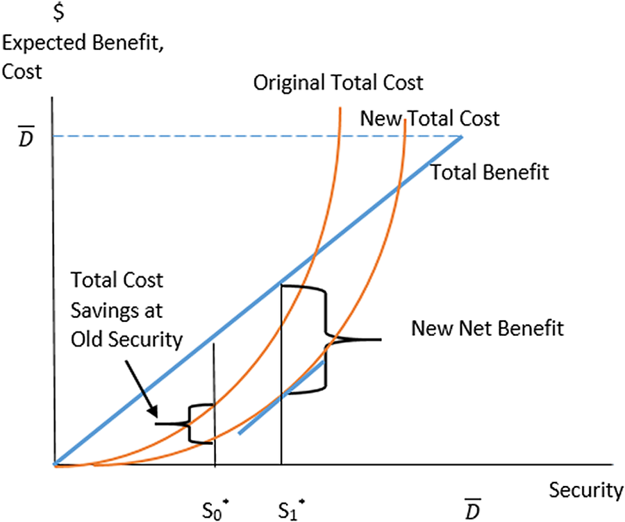
An organization is initially assumed to be carrying out operations at some baseline level. Figure 1 below displays the total expected net benefits and total costs. Security is on the horizontal axis, expected benefits and costs are on the vertical axis, and total benefits are shown as a 45° line equating security to the benefit (expected damages avoided). The expected benefits are zero if there is no security but at most can increase to a value equal to the maximum of damages avoided,
 $ \overline{D} $
, when there is perfect security. Numerous specifications for the cost function could meet the derivative requirements for what we assume is an interior optimum as we observe ongoing behavior. The quadratic and linear quadratic forms as defined in the Appendix provide a degree of linearity that is consistent with the level of detail in the data and are consistent with standard textbook treatments. The optimal level of security is found where the slope of the benefit and the cost lines are equal. The short blue line is tangent to the cost line at that quantity as illustrated. The maximum expected net benefit initially is at S0* in the diagram, with potentially quantifiable expected net benefits as indicated.
Initial optimal security from maximum expected net benefit.

2.2. Introducing a cost-saving technology
Assume that a new technology reduces costs at each possible level of security. The result in Figure 2 is a new total cost function. If decision-makers choose to maintain the same level of security, benefits result that are equal to the change in total cost at that original level of security, as illustrated. Assuming implementers act optimally, however, with typical cost functions they both reinvest the cost savings from the original security level and increase the level of spending in order to improve security. This suggests that using the cost savings would not just achieve a “break-even” scenario but also produce some positive rate of return. The new “optimal” level of security, S1*, provides an anchoring point for further analysis. The new net benefits are larger at the new level of security. A budget-constrained optimum is investigated later.
Cost savings at original security, and new net benefits at new security.

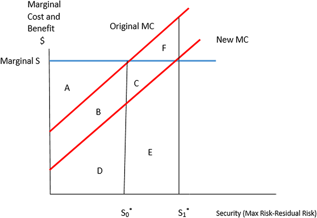
Focusing on incremental benefits and costs helps clarify the role of cost savings and additional security. The exact split between cost savings and new security benefits is developed using marginal analysis in Figure 3, with a quadratic cost function (second-order approximation) such that the marginal cost is linear, facilitating computation when data are sparse.Footnote 2 Derivative properties are unchanged from above.
Cost savings and net benefit with total cost (S) = aS + bS2; base technology in use.

The expected marginal benefit of a unit of security is $1, as security is denominated in dollars. The two optima are then found at the points of equivalency of the marginal values based on first-order conditions. The linear marginal cost form also allows welfare estimation from limited data using Harberger triangles as sufficient statistics (Harberger, Reference Harberger and Farrow2018).
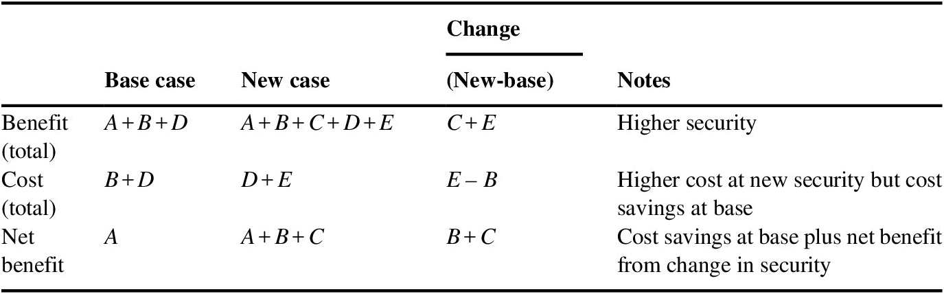
Further, using standard partial equilibrium benefit–cost representations (e.g., Boardman et al., Reference Boardman, D.H., A.R. and D.L.2018), letters can be used to represent areas (integrals) related to benefits and costs.Footnote 3 Table 1 above sets out the total benefits, total costs, net benefits, and changes in those values in moving from the base case to the new case. The bottom line expected net benefit to be estimated, area B + C, is comprised of two components gained in the use of the new technology. The first is the cost savings at the base case level of security. The second component is found in moving to the new level of security, an incremental net benefit (incremental expected benefit less incremental cost) that is to be added to the earlier cost savings. Note that the new incremental net benefit (area C) is not estimated by the incremental cost (area E) and also that area F has incremental costs that exceed incremental benefits beyond S0* when only the old technology is available. Area F is useful for estimation because, given the model assumptions, area C equals area F, and each is equal in value to one-half the change in security (length) times the change in incremental cost (height) for this parallelogram. Estimation using this approach will be presented in Section 4.
Benefit–cost by area when changing to new level of security.

We have sometimes been asked whether the cost savings in B must be “realized” by a budget reduction to be correct. Figure 3 illustrates why this is not necessary although it is possible. It shows an optimal situation where there are cost savings, B, but the same organization incurs additional costs, E, to achieve the security improvement. It may be that the costs in E are “internally” funded by the cost-savings of B, an organizational response we have observed. We also observed an organization realizing the cost-savings of B by reducing (or transferring) personnel. This does not appear to be optimal in the unconstrained case, but a suitably constrained problem might yield that behavior. However, given the assumptions above, the organization transferring resources to another task would appear to have foregone potential increases in security made more economic by the technological improvement. Consequently, we conclude that observing a budget reduction from realized cost savings is not necessary to generate real benefits and, in fact, a budget increase may be optimal.
The gains and losses from under- or over-investing in security (non-optimizing behavior) can also be seen in Figure 3. If the new level of security chosen is not “optimal” but to the left of the new optimum, then some of the incremental value of area C will be given up and the returns will be less than optimal. Conversely, if the level of security chosen is beyond the optimal level, then incremental costs exceed incremental benefits and the returns will also be less than optimal.Footnote 4
Implications of a budget-constrained optimum can also be inferred from Figure 3. In general, a budget-constrained optimum requires that net marginal benefits exceed a positive threshold represented by the shadow price of the budget constraint, λ (Farrow, Reference Farrow2007). In that case, the constrained optimum would be to the left of the appropriate unconstrained optima in Figure 3. The vertical distance between the marginal functions at the constrained optima equals λ0. With a new technology, even with the budget amount remaining constant, the net benefit function changes so that the new λ1 is not equal to the original λ 0, although the magnitude of the difference is a quantitative issue. If they were to be equal, it is an interesting result that with both new constrained optima to the left of their respective unconstrained optima, estimating area B + C as the welfare gain remains exactly correct.Footnote 5
3. Case studies
The empirical case studies involve the Los Angeles World Airports authority and the Federal Air Marshal Service, part of the Transportation Security Administration in DHS. In each case, new computer algorithms were combined with a game-theoretic approach to redirect resources, whether those resources were to establish vehicle inspection stops or to place armed security personnel onboard a flight (An & Tambe, Reference An and M.2017). Each context, including the baseline and organizational decision-making, is summarized below with further detail available at von Winterfeldt et al. (Reference von Winterfeldt, S., R, J., A. and H.2019) and Center for the Risk and Economic Analysis of Terrorism Events (CREATE) (2019).
3.1. Los Angeles International Airport/ARMOR
Los Angeles International Airport (LAX) has long been a target for terrorists. In addition to passenger screening, LAX security includes patrols and checkpoints, among other precautions. In the past, patrols and checkpoints were scheduled in a way that was fairly predictable, thus providing potential attackers an opportunity to observe the scheduled activities and seek targets that had no protection. The technological change involved the way that these activities were scheduled using Assistant for Randomizing Monitoring Over Routes (ARMOR). ARMOR uses a constrained optimization model, which provides a randomized schedule subject to different target values and other location constraints. As a software tool, ARMOR has been applied during the past 10 years at LAX to randomize checkpoints and canine patrols. Such implementation involved considerable interaction with LAX personnel, as described in Taylor et al. (Reference Taylor, C. and M.2011). Decision-makers at LAX determined that the main benefit of ARMOR was the reduction of staff costs while choosing to keep the level of security constant at the base level, as illustrated in Figure 2.
3.2. Federal Air Marshal Service/IRIS
Federal Air Marshal Service (FAMS) personnel fly semi-covertly on domestic and international flights, having been armed and trained to respond to in-flight terrorist attacks (Biles, Reference Biles2013; Stewart & Mueller, Reference Stewart and J.2013a, Reference Stewart and J.2013b). The baseline technology used human schedulers to assign air marshals to flights but was criticized as being imperfectly random at the same time that the scale of operations was increasing (US GAO, 2009, 2016). The Intelligent Randomization in Scheduling (IRIS) tool automates the international flight assignment process for air marshals while incorporating advanced randomization methods into the allocation process (Tsai et al., Reference Tsai, S., C., F., M., Decker, Sierra and Castelfranchi, unpaged.2009). The tool has been in use by FAMS since late 2009 and remains in use as of this writing. Decision-makers at FAMS have seen their budgets both increase and decrease over time, in part due to perceptions of risk, and appear to work to provide the greatest security given annual conditions.
4. Case study parametrization and results
The empirical challenge is to estimate the net benefits represented by area B + C or appropriate portions thereof. This area, the change in the net benefits per Table 1, is a sufficient statistic in that various primal functions such as conditional damages or marginal costs need not be measured. As an exercise, we might ask students to estimate the net benefits as area B, using the base level of security times the unit shift in cost, plus area C, using a one-half shift in cost, times the change in security were we to give them hypothetical data. To obtain actual data, we found that the agencies are most comfortable evaluating expenditures. Consequently, rather than trying to estimate changes in security directly, we asked about anchoring points and changes in expenditures or share of expenditures from that anchoring point to reach the new level of security. Two examples are provided below prior to the specifics for the two cases.
-
(i) Example method 1: Cost savings only, no increase in security. If the agency or subject matter experts indicate that there was no increase in security because fewer resources were used to achieve the same level of security, then area C is zero and one uses information to estimate the cost savings actually achieved. This was the situation with LAX/ARMOR, where the agency and research indicated they could deliver the original level of security at about 50 % of the cost using the new technology (more below).
-
(ii) Example method 2: Cost savings plus additional security. One approach is to estimate both proportional cost savings from the new technology and the relative increase in security. In the retrospective case of IRIS, baseline expenditures (B + D) prior to IRIS were known as well as expenditures with IRIS in each period (D + E). The question was asked of FAMS personnel about proportional total cost savings (B + C + F) compared to expenditures with IRIS (D + E) to achieve the new level of security and combined with modeled results for the relative increase in security as developed further below. As expenditures change each year the benefits change. If the change is due to changes in risk, as some were stated to be, then the resulting expenditure adjustment is assumed to restore optimality by moving along the marginal cost function. Deviations from optimality caused by over or under-expenditure for other reasons are discussed above (following Table 1) such that the unconstrained optimal net benefit estimates reported here would overstate the actual net benefits.Footnote 6 However, ideal adjustments to the net benefits in the neighborhood of the optimum would likely be small for the reasons discussed above.
The two cases studied here are part of a larger group of case studies using expected value models to estimate the rate of return to research investments (CREATE, 2018, 2019). All the case studies, including those described here, used some common parameters and analytical conditions. All studies evaluated a 10-year return, which, for most case studies, occurred in the future. A few case studies were retrospective, as with ARMOR, and some had a mix of retrospective and prospective elements, as with IRIS. Prospective benefits and costs were discounted in a standard manner guided by discount rates used for U.S. Government evaluations (US OMB, 2003). The prospective discount rate for the base case is 3 % (real) with a triangular distribution used for simulations of 0, 3, and 7 % (real) where 7 % is a higher federally identified rate and 0 as the non-negative bound. These rates, while subject to debate, are taken as averages of different opportunity costs (US Council of Economic Advisers, 2017).
The treatment of retrospective values adhered to the principle of using values that actually occurred. Retrospective values, including the nominal costs of federal government investment, must be brought forward to the present value year (here 2017). Such “future valuing” of nominal values requires both an actual inflation factor and an actual real interest rate; or a suitable historical nominal rate of interest which includes both factors (Howard, Reference Howard2017). Our approach, in part for transparency regarding inflation, was to separate the nominal interest rate into its inflation and real interest components. For the inflation component we used the consumer price index (CPI) to adjust for price changes to the desired year. For the real interest rate component, we researched the actual real federal borrowing rate recommended for cost saving government investments (US OMB, 1992, 2019) and determined that for this specific historical period following the Great Recession, the real federal borrowing rate was appropriately averaged as zero (see also US Council of Economic Advisors, 2017). In some of these historical periods, the actual real rate was negative and others had relatively low positive values. Taking both factors together, nominal values from the specific retrospective period were brought forward at a nominal interest rate that simplified to the rate of inflation. We note that this is not a general result but was consistent with the retrospective facts.
Other parameters used in some case studies, such as the value of a statistical life, were not necessary for the cases discussed here, another advantage of bypassing explicit estimation of damages. Each case study from the larger set reported results for the NPV and rate of return for the base case, break-even, sensitivity and Monte Carlo simulation analyses. Costs were obtained from the universities carrying out the research and the organizations implementing the technology (see CREATE, 2018, 2019; von Winterfeldt et al., Reference von Winterfeldt, S., R, J., A. and H.2019). The context for each case differs, such as the quantity with which to determine the break-even NPV. Sensitivity analyses were carried out, with agency- and literature-informed subjective bounds for key variables determining net benefits; results are presented using a tornado diagram showing deviations in outcomes from the base case for each uncertain variable. Triangular distributions, using the bounds and most likely value from the sensitivity analysis, were used in the simulations running 10,000 trials.Footnote 7 The two cases reported on here use the same assumptions and report the same result metrics but with limited attention to ARMOR as more detail is published in von Winterfeldt et al. (Reference von Winterfeldt, S., R, J., A. and H.2019) but FAMS/IRIS is a new case reported more completely here.
4.1. LAX/ARMOR case
Before ARMOR was implemented at LAX, there were six checkpoints and four teams of five officers each assigned to these checkpoints. These teams moved between the six checkpoints according to a fixed schedule. For reasons unrelated to ARMOR, the number of checkpoints was reduced to four in 2006. When ARMOR was introduced, it was determined that two teams assigned to the four checkpoints with ARMOR was sufficiently protective of LAX targets, thus reducing staffing from four teams to two teams. This conclusion was based on a calculation of the security level afforded by both the prior non-random schedule and the new schedule, determined by an optimization of the security level based on constrained randomization and the values of the protected targets (Jain et al., Reference Jain, J., J., C., S., F. and M.2012; An & Tambe, Reference An and M.2017).
Cost savings were based on maintaining the initial security level as informed by the expected value of having a checkpoint or patrol at a target location (in this case, a terminal at LAX) and considering the value of the target. For example, the Bradley International terminal was assigned a higher value by Los Angeles Airport Police staff than all other terminals, due to the level of traffic and past attacks at that terminal. Prior to the implementation of ARMOR, checkpoints and patrols did not consider the target value and were not randomized. ARMOR, in contrast, led to longer and more frequent checks and patrols at higher value targets. Thus, the expected value of protecting possible targets (security) could be increased, roughly by a factor of two, so that the initial level of security could be maintained at about 50 % of the cost using the new technology (Taylor et al., Reference Taylor, C. and M.2011).
The reduction of the staff costs while maintaining the same protective value resulted in a substantial cost savings that could be calculated based on staffing costs, while some small amount of benefit was allocated for drug and gun seizures. To break even by recouping the $1 million cost of developing and implementing ARMOR, it would be sufficient to eliminate one of the four original checkpoint teams for about 9 months at regular pay rates, and even less if overtime rates are paid. Benefits per year were $3.2 million (in 2017 dollars), of which over 95 % was the result of cost savings. The present value net benefit is about $30.7 million for 10 years of use. The benefit-to-cost ratio is 30.07, and the return on investment (ROI) is 2907 %. Table 2 presents these results.
Estimated base case benefits and NPV for ARMOR (million 2017 dollars).

Abbreviation: PV, present value; NPV, net present value.
Sensitivity analysis carried out through a tornado diagram indicated that the percentage of overtime pay for staffing before and after implementation of ARMOR has a major impact, as does the number of years of ARMOR implementation. By comparison, the valuation of drug and weapons seizures has a relatively small impact, which is why this case is characterized by cost savings. Monte Carlo simulation analysis was implemented as discussed above, although not all triangular distributions were symmetric, and resulted in a distribution of net benefits where the 5th, 50th, and 95th percentiles are $25.4, $29.0, and $32.2 million, respectively, with a mean value of $28.9 million (standard deviation, $2.0 million).
4.2. FAMS/IRIS case
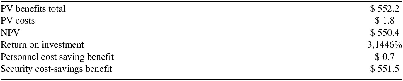
The FAMS average nominal budget in the study period was about $850 million per year. Cost-saving benefits result from both a shift from a labor-intensive scheduling process in international operations to an automated process and through improved security at all expenditure levels from improved randomization. Improved security will be shown to be the larger component of benefits. Regarding labor savings, at the base level of assignments in 2009, FAMS estimates that IRIS saved 25 % of the wage and benefits cost of a full-time equivalent employee (FTE), (FAMS personal communication, 2018). For this and later personnel-related analysis, FAMS provided an estimate of the full cost of an FTE at $150,000 in 2017 dollars, resulting in $37,500 in savings per year (in 2017 dollars). In addition, the assignment workload has generally been larger but variable since 2009, when IRIS was first implemented. FAMS reported that a 50 % increase in assignments would lead to additional cost savings over the baseline of 50 % of an FTE, a 1 % increase in cost savings for each per cent increase in assignments. While the number of personnel or assignments are unknown, FAMS provided information on expenditures related to assignments for each year. Consequently, additional cost savings as a fraction of an FTE were recorded for each year based on the change in assignment expenditures as compared to the base year. While incorporated in a later table, these two cost-saving benefits total $0.7 million in present value 2017 dollars.
With regard to the value of improving security, relatively extensive evaluation testing has been carried out on IRIS and on a family of models similar to IRIS (Taylor et al., Reference Taylor, C. and M.2011, Reference Taylor, C., E., F. and M.2017; An & Tambe, Reference An and M.2017). The source of improved security is improved randomization compared to original practice. Some tests identify relative improvements of different defensive strategies given the assumptions of the models. Other approaches include expert testimony, red-team testing, and so on. Taylor et al. (Reference Taylor, C. and M.2011, Reference Taylor, C., E., F. and M.2017) indicate that further testing was done within FAMS in a classified manner to which they were not privileged. The approach used here for the security benefits of IRIS begins with an estimate from FAMS of the expenditures that would have been necessary in the baseline technology to achieve the security provided by IRIS through its improved randomization procedures, as discussed in conjunction with Figure 3. It would have been possible both to achieve the older level of security at a lower cost due to improved randomization and to realize some improvement in security since FAMS expenditures have not fallen below the 2008 level. FAMS provided an estimate of the proportional increase in international expenditures, with uncertainty ranges, for the total amount in the benefit–cost areas B + C + F, the difference between the two incremental cost lines of Figure 3. No official estimates of the international expenditures as a proportion of total FAMS expenditures exist, although international flights are frequently mentioned in the literature as an important component. It is assumed here that the international expenditures represent 50 % of total FAMS expenditures, with an uncertainty range from 25 to 75 %. Area F should be deducted from the gross savings estimate obtained by the product of the international expenditures and the security cost-saving proportion from IRIS. Using additional information on the proportional improvement in security from modeling tests (Taylor et al., Reference Taylor, C. and M.2011, Reference Taylor, C., E., F. and M.2017), we estimate that IRIS provides an increase in security of 32 % compared to the baseline process. This estimate is somewhat more than the approximately 20 % increase in security reported as the gain from IRIS compared to a well-implemented uniform statistical randomization (Tsai et al., Reference Tsai, S., C., F., M., Decker, Sierra and Castelfranchi, unpaged.2009). This information is sufficient to estimate the cost savings of improved security (area B + C) as gross cost savings times one minus the product of one-half times the estimated proportional increase in security from the modeling tests. As there is large uncertainty about the estimated increase in security, the uncertainty analysis to follow uses an upper bound of a 64 % increase in security in the absence of operational constraints and a lower bound of 0, assuming that operational constraints totally offset the security benefits in conjunction with the modal estimate of 32 %.
FAMS reported an estimate that it would have taken 15 % more of their total international program expenditures to achieve the new level of security (with a minimum and maximum being plus or minus 75 % of that figure). Deducting the base case mean proportion of area F reduces this datum to about 12.6 %. The resulting security benefits were generated on a year-by-year basis and converted to present value 2017 dollars. The annual benefits averaged about $56.2 million per year, for total present value benefits of $552.2 million in 2017 dollars over the 10-year period. Almost all the benefits, $551.5 million, resulted from improved randomization, although there are $0.7 million in benefits from personnel cost savings (details may not add to total due to rounding).
Table 3 below presents the base case NPV for the analysis, including the breakdown between cost savings for scheduling personnel and those from improved randomization.
Estimated base case benefits and NPV for IRIS (million 2017 dollars).

Abbreviation: IRIS, Intelligent Randomization in Scheduling; PV, present value; NPV, net present value.
Source: CREATE (2019)
Given the base case inputs and the present value (in 2017 dollars) of the costs and the benefits of the analysis, the estimated NPV of using IRIS is $550.4 million. This results in a base case ROI of 31,446 %, meaning that IRIS is estimated to have returned, on net, about 314 times its cost in present value terms. More familiar in benefit–cost practice is the benefit–cost ratio, 315, as it does not deduct the Present Value (PV) cost in the numerator.
4.2.1. Break-even and sensitivity analysis
Several different break-even analyses are carried out. A key driver of benefits is the percentage increase FAMS would have had to spend to achieve the same level of security as with IRIS. Allowing that percentage to change while holding costs and other cost savings constant results in a break-even estimate of 0.02 %. In other words, if FAMS estimated they could have achieved the same new level of security using the old system by increasing its costs by 0.02 % (one-fifth of one per cent), then the costs of IRIS would have been repaid. Using a different type of analysis, DHS has sometimes used an investment-to-cost ratio to define the change in probability necessary to break even (Farrow & Shapiro, Reference Farrow and S.2009). Using data for the cost of IRIS and the consequence used by Steward and Mueller (2013), that reduction in probability is 0.0035 %, a relatively small number.
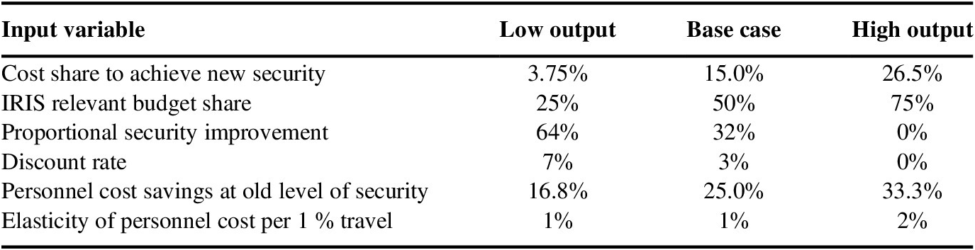
The costs of developing and transitioning IRIS are relatively well known, but many of the parameters affecting benefits are quite uncertain. Table 4 below summarizes the parameter values for these variables. The direction of impact (slope) is indicated by High or Low Output. For instance, a high cost share (26.5 %) to achieve the new security level results in a high NPV, but a high proportional security improvement (64 %) results in the low NPV case. The latter result occurs because the higher the security improvement percentage, the more that is subtracted as area F in Figure 3.
Ranges of IRIS inputs for sensitivity analysis.

Abbreviation: IRIS, Intelligent Randomization in Scheduling; NPV, net present value.
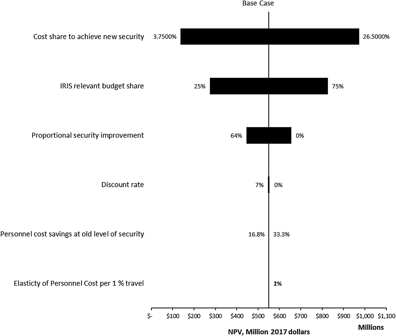
The key determinants of NPV are investigated by applying a structured sensitivity approach, using data in Table 4. Figure 4 presents these results as a tornado diagram, which is created by calculating the NPV (shown as million 2017 dollars) at the low parameter value of Table 4 and the high value and plotting the difference as a horizontal bar of NPVs. The base case value is shown as a vertical line. This is done one variable at a time (no interactions). The bars are presented in descending order of length, creating the image of a tornado, with high NPV impact variables on the top and low impact variables at the bottom.
Net present value (NPV) tornado diagram—Intelligent Randomization in Scheduling (IRIS).

Given these ranges of uncertainty, both the proportional cost to achieve the new level of security using the old technology and the share of FAMS budget to which IRIS is applied – the international scheduling component – are seen to be key determinants of the NPV. Increases from the base case for both variables increase the NPV, and vice versa. Uncertainty in the other parameters are shown to have a relatively smaller impact on NPV, although all low output (NPV) tests result in a positive NPV.
4.2.2. Uncertainty and simulation
To further explore the uncertainties of some of the input variables, we assumed that these uncertainties can be characterized by triangular distributions with values from Table 4. The analysis assumes that all input variables are independent and thus uncorrelated with each other.
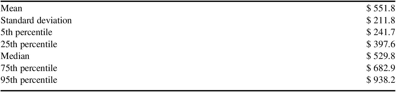
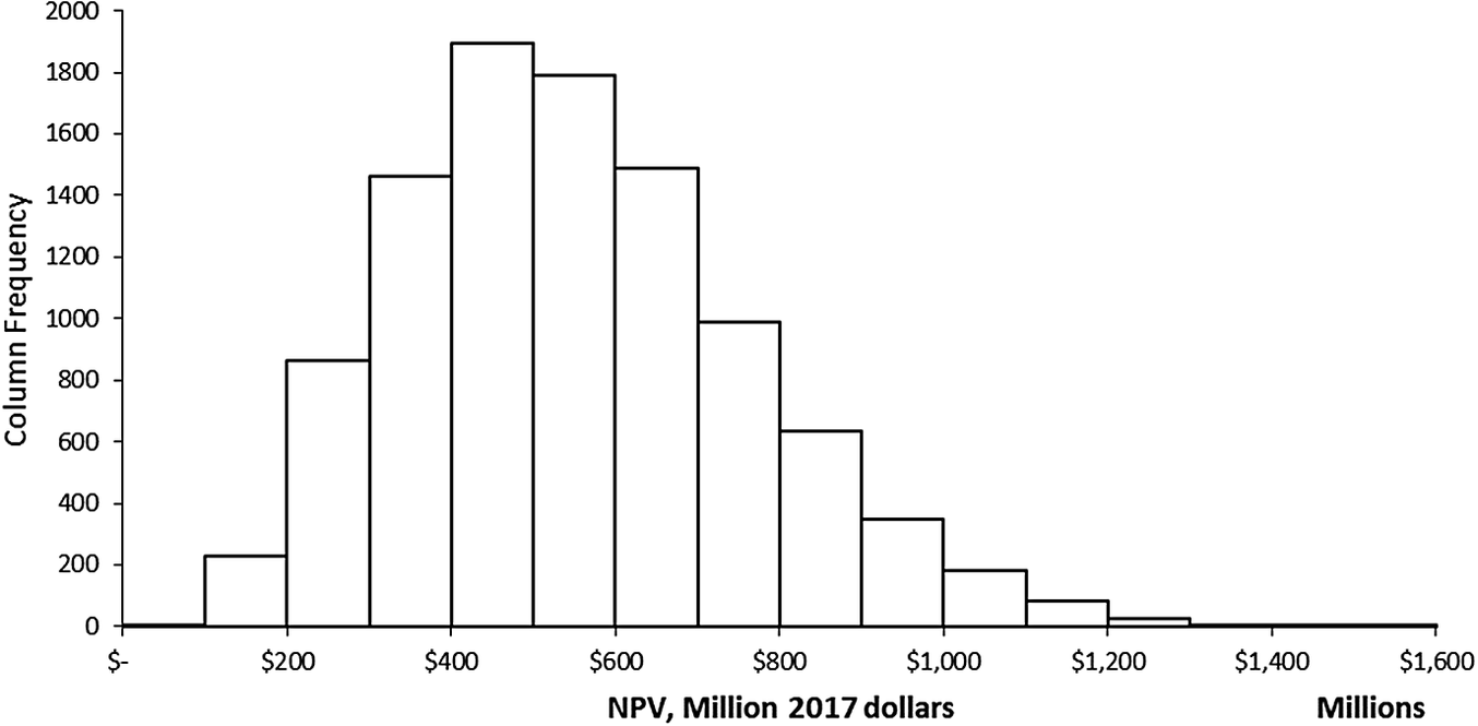
Table 5 presents results of the simulation for the NPV from IRIS, while Figure 5 charts a more detailed histogram of those results. The mean, median, 5th percentile, and 95th percentile NPV values are $551.8 million, $529.8 million, $241.7 million, and $938.2 million, respectively, all in 2017 present value dollars.
Statistics of the IRIS NPV distribution (million 2017 dollars).

Abbreviation: IRIS, Intelligent Randomization in Scheduling; NPV, net present value.
Source: CREATE (2019)
IRIS simulation results for the net present value, in million 2017 dollars.

There were no negative values in the simulation with the “worst” individual simulated case being a positive $83.5 million (not shown in Table 5). However, the parameter values for this lowest NPV value can be investigated as to how close it may have been to a “worst case” scenario defined by the lower bound on all uncertain variables (see Figure 1). The lowest estimated NPV case had parameter values of: (i) Cost Share Achieve New Security at 4 %, 0.25 % above its lower bound, (ii) Budget Share at 25 %, its lower bound, but (iii) Security Improvement at 0 %, its upper bound with all other variables having small impact on the NPV as seen in Figure 1. As the total “swing” in the NPV from the range in the Security Improvement variable in the base case is $210 million, it is conceivable that that the lowest estimated NPV could have been negative for the worst simulated case estimated. However, an actual “worst case” scenario using all parameter values at their lowest NPV effect value, resulted in an NPV of $55.4 million (2017 dollars). This “worst case” is outside the Monte Carlo bounds and an indication of the non-linear interaction of variables, particularly far away from the mean value such that the effect of the swing in the security improvement was attenuated compared to its evaluation at the mean.
Different distributional assumptions can also affect the result. However, assuming a uniform distribution would not affect the mean as the FAMS provided ranges (for all variables except the discount rate) are symmetric around the mode, thus the mean value would be preserved while giving somewhat more weight to both higher and lower values. The distribution for the discount rate, while slightly skewed high, would only slightly increase the discount rate from 3 to 3.5 % were a uniform distribution assumed. Such a change would only apply to the 2 years that are “prospective” in this analysis and so result in only a slightly smaller net present value. Ultimately, while the uncertainty analysis substantially spreads the estimated value of the NPV from IRIS, the returns are estimated to be large.Footnote 8
5. Conclusion
Homeland security investments have been resistant to the application of benefit–cost analysis due to challenges in estimating risk or its complement, security. Cases involving technological change might be seen as adding new complications. However, modeling a change from an existing baseline reduces some computational issues, and defining output as security facilitates using expenditure-based information from subject matter experts. The conceptual model developed here, while retaining limitations of rationality and linearity in marginal functions, allows net benefits to be estimated from sparse data. The conceptual model is applied to two different cases: (i) changes to checkpoints and patrols using ARMOR and (ii) changes to the assignment of armed personnel on commercial flights using IRIS. Each technological change is retrospectively estimated to have very large net present values and benefit–cost ratios, indicating that they were a net beneficial investment.
The main lesson from these applications were that in the simple case of cost savings at a given security level, the application of benefit cost analysis is straightforward. However, structurally estimating the benefits from increased security is extremely complex due to the difficulties in estimating the baseline and reduced security risks (probabilities and the degree of consequence with and without the new technology). Our primary model shows that, under given rationality assumptions, it is sufficient to know the relative risk reduction (e.g., an expected per cent change in the probability or consequence) and expenditure information to evaluate the benefits of a new technology. An alternative approach that drops the assumption of reaching a second optimum but merely reinvests the cost savings at the original level of security can yield estimates without estimating the relative increase in security. These approaches provide new opportunities to apply benefit–cost analysis to evaluating security projects and to guide investment decisions by security R&D managers.
Supplementary Materials
To view supplementary material for this article, please visit http://dx.doi.org/10.1017/bca.2020.24.
Acknowledgments
Appreciation is extended to seminar participants at the Society for Benefit–Cost Analysis, the Marine Policy Center of the Woods Hole Oceanographic Institution, and the University of Southern California. We thank especially Milind Tambe, Manish Jain (of AVATA, Inc.), Richard John and three referees. The work would not have been possible without the knowledge and assistance of personnel at the Los Angeles International Airport, the Coast Guard, and the Federal Air Marshal Service, although modeling and results are the responsibility of the authors. The work was performed under Basic Ordering Agreement HSHQDC-10-BOA19/HSHQDC-16-J-00467 with the Department of Homeland Security.