1 Introduction
Turbulence is a ubiquitous phenomenon that spans a broad range of temporal and spatial scales. In a turbulent system energy is transferred from large (or ‘energy-containing’) eddies to small eddies, ultimately resulting in production of internal energy or heat by dissipation. This process of energy cascade is observed in turbulent neutral fluids as well as turbulent plasmas. The rate of energy decay in a turbulent system is both an interesting problem (Kolmogorov Reference Kolmogorov1941) and also an important practical one. In laminar flows the rate of energy loss is determined by the molecular viscosity of the fluid, but in a turbulent system the energy dissipation rate appears to become independent of viscosity and approach a non-zero value as the fluid becomes increasingly turbulent (Onsager Reference Onsager1949). Taylor (Reference Taylor1938) gave an empirical expression for the energy decay rate of turbulent neutral fluids. This analytical expression can be obtained from the work of de Kármán & Howarth (Reference de Kármán and Howarth1938) by assuming the preservation of the shape of the two-point velocity correlation function during turbulent decay (Dryden Reference Dryden1943).
Energy decay in plasmas is a more complicated problem. Magnetohydrodynamic (MHD) theory is the simplest extension of hydrodynamic turbulence theories to conducting fluids and the decay of energy-containing eddies in MHD turbulence has been the subject of various studies (e.g., Hossain et al.
Reference Hossain, Gray, Pontius, Matthaeus and Oughton1995, Reference Hossain, Gray, Pontius, Matthaeus and Oughton1996; Linkmann et al.
Reference Linkmann, Berera, McComb and McKay2015; Linkmann, Berera & Goldstraw Reference Linkmann, Berera and Goldstraw2017). Note that the presence of an external mean magnetic field,
 $\boldsymbol{B}_{0}$
, makes the problem of energy decay in MHD more complex because the mean-field introduces anisotropy in the system (Robinson & Rusbridge Reference Robinson and Rusbridge1971; Montgomery & Turner Reference Montgomery and Turner1981; Montgomery Reference Montgomery1982; Shebalin, Matthaeus & Montgomery Reference Shebalin, Matthaeus and Montgomery1983; Oughton, Priest & Matthaeus Reference Oughton, Priest and Matthaeus1994; Hossain et al.
Reference Hossain, Gray, Pontius, Matthaeus and Oughton1995).
Energy cascade through the MHD inertial scales is given by a Kolmogorov–Yaglom (Kolmogorov Reference Kolmogorov1941; Monin & Yaglom Reference Monin and Yaglom1975) third-order law extended to MHD (Politano & Pouquet Reference Politano and Pouquet1998a ,Reference Politano and Pouquet b ). On average, the energy transfer rate associated with cascading of excitation from the large scales (determined by the von Kármán-type phenomenology) and the energy cascade rate associated with inertial range scales (given by the third-order law) are expected to be in agreement (Kolmogorov Reference Kolmogorov1941; Batchelor Reference Batchelor1953; Bandyopadhyay et al. Reference Bandyopadhyay, Chasapis, Chhiber, Parashar, Matthaeus, Shay, Maruca, Burch, Moore and Pollock2018).
The problem of similarity decay in isotropic and anisotropic incompressible MHD turbulence is studied in detail by Wan et al. (Reference Wan, Oughton, Servidio and Matthaeus2012), where it is shown that similarity solutions are possible in MHD. However, unlike the situation for isotropic neutral fluids, universality, even at asymptotically high Reynolds number, is not expected for MHD due to potential variation of other parameters such as magnetic Prandtl number, cross-helicity, magnetic helicity and Alfvén ratio. Thus one might anticipate that in MHD the conditions for obtaining similarity solutions are more restrictive. Indeed, Wan et al. (Reference Wan, Oughton, Servidio and Matthaeus2012) shows, analytically, that a similarity solution for MHD fluid with a mean magnetic field is possible only if, during the similarity decay, the similarity length scale parallel to the mean field remains proportional to the similarity length scale perpendicular to the mean-field. As far as we are aware, whether the two length scales remain in constant proportion has not yet been tested in simulations or experiments. This motivates the present study. We will discuss results from a set of (spectral method) numerical MHD turbulence experiments that examine the dynamical behaviour of the ratio of the parallel and perpendicular correlation scales. This enables us to assess whether or not a similarity decay phase occurs in anisotropic three-dimensional (3-D) MHD in the presence of a mean magnetic field (Wan et al. Reference Wan, Oughton, Servidio and Matthaeus2012). The results confirm, perhaps surprisingly, that the required condition for similarity decay of anisotropic MHD can be satisfied.
2 Theory
In this section we briefly review the Wan et al. (Reference Wan, Oughton, Servidio and Matthaeus2012) derivation of similarity decay phenomenology for anisotropic MHD with a mean magnetic field. As in that work, we take the mass density to be constant and set it to unity. We denote the fluctuating velocity and magnetic fields by
 $\boldsymbol{v}$
and
 $\boldsymbol{b}$
, respectively. Without loss of generality, we take the mean magnetic field as
 $\boldsymbol{B}_{0}=B_{0}\hat{\boldsymbol{z}}$
. All magnetic fields are converted to Alfvén units. The equations of incompressible MHD can be written in terms of Elsasser variables for the fluctuations,
 $\boldsymbol{z}^{\pm }=\boldsymbol{v}\pm \boldsymbol{b}$
, as
 $$\begin{eqnarray}\frac{\unicode[STIX]{x2202}\boldsymbol{z}^{\pm }}{\unicode[STIX]{x2202}t}=-\boldsymbol{z}^{\mp }\boldsymbol{\cdot }\unicode[STIX]{x1D735}\boldsymbol{z}^{\pm }\pm \boldsymbol{B}_{0}\boldsymbol{\cdot }\unicode[STIX]{x1D735}\boldsymbol{z}^{\pm }-\unicode[STIX]{x1D735}P+\unicode[STIX]{x1D708}\unicode[STIX]{x1D6FB}^{2}\boldsymbol{z}^{\pm },\end{eqnarray}$$
where
 $P$
is the total (magnetic
 $+$
kinetic) pressure, and
 $\unicode[STIX]{x1D708}$
is the viscosity, for simplicity assumed to be equal to the resistivity herein.
The second-order correlation tensors for the corresponding Elsasser fields are defined as
 $$\begin{eqnarray}\unicode[STIX]{x1D619}_{ij}^{\pm }(\boldsymbol{r},t)=\langle z_{i}^{\pm }(\boldsymbol{x},t)z_{j}^{\pm }(\boldsymbol{x}+\boldsymbol{r},t)\rangle ,\end{eqnarray}$$
where
 $\langle \cdots \rangle$
denotes an ensemble average. Using the MHD equations one can derive the following equation for the time evolution of the traced second-order correlation function
 $$\begin{eqnarray}\frac{\unicode[STIX]{x2202}}{\unicode[STIX]{x2202}t}\unicode[STIX]{x1D619}_{ii}^{\pm }(\boldsymbol{r},t)=-\frac{\unicode[STIX]{x2202}}{\unicode[STIX]{x2202}r_{k}}[\hat{Q}_{k}^{\pm }(\boldsymbol{r},t)-\hat{Q}_{k}^{\pm }(-\boldsymbol{r},t)]+2\unicode[STIX]{x1D708}\frac{\unicode[STIX]{x2202}^{2}\unicode[STIX]{x1D619}_{ii}^{\pm }}{\unicode[STIX]{x2202}r_{k}\unicode[STIX]{x2202}r_{k}}.\end{eqnarray}$$
Here
 $$\begin{eqnarray}\hat{Q}_{k}^{\pm }(\boldsymbol{r},t)=\langle z_{k}^{\mp }(\boldsymbol{x}+\boldsymbol{r},t)z_{i}^{\pm }(\boldsymbol{x},t)z_{i}^{\pm }(\boldsymbol{x}+\boldsymbol{r},t)\rangle\end{eqnarray}$$
is a triple correlation. It is interesting that the mean magnetic field
 $\boldsymbol{B}_{0}$
does not appear explicitly in (2.3), despite the well known fact that these correlation functions (and their Fourier transforms, the Elsasser energy spectra) do display anisotropy relative to
 $\boldsymbol{B}_{0}$
. In fact, the first explicit appearance of a mean magnetic field in the correlation function hierarchy is in the equation for evolution of the third-order correlations (Wan et al.
Reference Wan, Oughton, Servidio and Matthaeus2012; Oughton et al.
Reference Oughton, Wan, Servidio and Matthaeus2013). Consequently, the dynamical influence of
 $\boldsymbol{B}_{0}$
is exerted on (2.3) through the structure of the third-order correlations. Therefore, the limit of large
 $\boldsymbol{B}_{0}$
that permits reduction to quasi-two-dimensional MHD must occur in those higher order equations, and not directly in (2.3).
A set of similarity solutions can be derived from these equations using a heuristic scaling argument, as shown by de Kármán & Howarth (Reference de Kármán and Howarth1938) for hydrodynamic turbulence and generalized to MHD by Wan et al. (Reference Wan, Oughton, Servidio and Matthaeus2012). Here, we outline the steps only for the case of anisotropic MHD decay in the presence of a mean magnetic field. It is well established that a mean magnetic field affects the dynamics of the dissipation rate in a turbulent system (e.g., Shebalin et al.
Reference Shebalin, Matthaeus and Montgomery1983; Oughton et al.
Reference Oughton, Priest and Matthaeus1994; Bigot, Galtier & Politano Reference Bigot, Galtier and Politano2008a
,Reference Bigot, Galtier and Politano
b
). Without loss of generality, we allow for non-zero cross-helicity
 $H_{c}=\langle \boldsymbol{v}\boldsymbol{\cdot }\boldsymbol{b}\rangle$
. The zero cross-helicity case is recovered as a special solution.
Assuming the system to be axisymmetric with respect to the mean-field direction
 $\hat{\boldsymbol{z}}$
, we write the second-order correlation functions in the form
 $$\begin{eqnarray}\unicode[STIX]{x1D619}_{ii}^{\pm }(\boldsymbol{r},t)=\unicode[STIX]{x1D619}_{ii}^{\pm }(r_{\Vert },r_{\bot },t),\end{eqnarray}$$
where
 $r_{\Vert }=\boldsymbol{r}\boldsymbol{\cdot }\hat{\boldsymbol{z}}$
and
 $r_{\bot }=|\boldsymbol{r}-r_{\Vert }\hat{\boldsymbol{z}}|$
. Clearly,
 $r_{\Vert }$
and
 $r_{\bot }$
are equivalent to the height
 $(z)$
and radial
 $(s)$
coordinates in the usual cylindrical polar coordinate system
 $(s,\unicode[STIX]{x1D719},z)$
. Using the theory of axisymmetric tensors (Batchelor Reference Batchelor1953; Politano, Gomez & Pouquet Reference Politano, Gomez and Pouquet2003), the triple correlations can be written as
 $$\begin{eqnarray}\displaystyle & \hat{Q}_{k}^{\pm }(\boldsymbol{r},t)=A^{\pm }(r_{\Vert },r_{\bot },t)\hat{r}_{k}+C^{\pm }(r_{\Vert },r_{\bot },t)\hat{\boldsymbol{z}}, & \displaystyle\end{eqnarray}$$
 $$\begin{eqnarray}\displaystyle & \hat{Q}_{k}^{\pm }(-\boldsymbol{r},t)=-A^{\pm }(-r_{\Vert },r_{\bot },t)\hat{r}_{k}+C^{\pm }(-r_{\Vert },r_{\bot },t)\hat{\boldsymbol{z}}. & \displaystyle\end{eqnarray}$$
Inserting expressions (2.6)–(2.7) into (2.3) yields
 $$\begin{eqnarray}\unicode[STIX]{x2202}_{t}\unicode[STIX]{x1D619}_{ii}^{\pm }=-\left(\frac{\unicode[STIX]{x2202}A_{2}^{\pm }}{\unicode[STIX]{x2202}r_{\bot }}\frac{r_{\bot }}{r}+\frac{\unicode[STIX]{x2202}A_{2}^{\pm }}{\unicode[STIX]{x2202}r_{\Vert }}\frac{r_{\Vert }}{r}+\frac{2A_{2}^{\pm }}{r}+\frac{\unicode[STIX]{x2202}C_{2}^{\pm }}{\unicode[STIX]{x2202}r_{\Vert }}\right)+2\unicode[STIX]{x1D708}\left(\frac{\unicode[STIX]{x2202}^{2}\unicode[STIX]{x1D619}_{ii}^{\pm }}{\unicode[STIX]{x2202}r_{\bot }^{2}}+\frac{1}{r_{\bot }}\frac{\unicode[STIX]{x2202}\unicode[STIX]{x1D619}_{ii}^{+}}{\unicode[STIX]{x2202}r_{\bot }}+\frac{\unicode[STIX]{x2202}^{2}\unicode[STIX]{x1D619}_{ii}^{\pm }}{\unicode[STIX]{x2202}r_{\Vert }^{2}}\right),\end{eqnarray}$$
where
 $$\begin{eqnarray}\displaystyle & A_{2}^{\pm }(r_{\Vert },r_{\bot },t)=A^{\pm }(r_{\Vert },r_{\bot },t)+A^{\pm }(-r_{\Vert },r_{\bot },t), & \displaystyle\end{eqnarray}$$
 $$\begin{eqnarray}\displaystyle & C_{2}^{\pm }(r_{\Vert },r_{\bot },t)=C^{\pm }(r_{\Vert },r_{\bot },t)-C^{\pm }(-r_{\Vert },r_{\bot },t), & \displaystyle\end{eqnarray}$$
with
 $A_{2}^{\pm }(-r_{\Vert },r_{\bot },t)=A_{2}^{\pm }(r_{\Vert },r_{\bot },t)$
and
 $C_{2}^{\pm }(-r_{\Vert },r_{\bot },t)=C_{2}^{\pm }(r_{\Vert },r_{\bot },t)$
.
Following de Kármán & Howarth (Reference de Kármán and Howarth1938) and Wan et al. (Reference Wan, Oughton, Servidio and Matthaeus2012) we assume
 $$\begin{eqnarray}\displaystyle & \unicode[STIX]{x1D619}_{ii}^{+}(\boldsymbol{r},t)=Z_{+}^{2}\,f(\unicode[STIX]{x1D702}_{\Vert },\unicode[STIX]{x1D702}_{\bot }), & \displaystyle\end{eqnarray}$$
 $$\begin{eqnarray}\displaystyle & A_{2}^{+}(\boldsymbol{r},t)=Z_{-}Z_{+}^{2}a(\unicode[STIX]{x1D702}_{\Vert },\unicode[STIX]{x1D702}_{\bot }), & \displaystyle\end{eqnarray}$$
 $$\begin{eqnarray}\displaystyle & C_{2}^{+}(\boldsymbol{r},t)=Z_{-}Z_{+}^{2}c(\unicode[STIX]{x1D702}_{\Vert },\unicode[STIX]{x1D702}_{\bot }). & \displaystyle\end{eqnarray}$$
introducing the normalized variables
 $\unicode[STIX]{x1D702}_{\Vert }=r_{\Vert }/L_{\Vert }^{+}(t)$
and
 $\unicode[STIX]{x1D702}_{\bot }=r_{\bot }/L_{\bot }^{+}(t)$
, and the shorthand notation
 $Z_{\pm }^{2}=\unicode[STIX]{x1D619}_{ii}^{\pm }(0,t)=\langle |\boldsymbol{z}_{\pm }|^{2}\rangle$
. Using (2.11)–(2.13), in (2.8) we obtain
 $$\begin{eqnarray}\displaystyle & & \displaystyle \left\{\frac{\text{d}Z_{+}^{2}}{\text{d}t}\right\}[f]-\left\{\frac{Z_{+}^{2}}{L_{\Vert }^{+}}\frac{\text{d}L_{\Vert }^{+}}{\text{d}t}\right\}\left[\frac{\unicode[STIX]{x2202}f}{\unicode[STIX]{x2202}\unicode[STIX]{x1D702}_{\Vert }}\unicode[STIX]{x1D702}_{\Vert }\right]-\left\{\frac{Z_{+}^{2}}{L_{\bot }^{+}}\frac{\text{d}L_{\bot }^{+}}{\text{d}t}\right\}\left[\frac{\unicode[STIX]{x2202}f}{\unicode[STIX]{x2202}\unicode[STIX]{x1D702}_{\bot }}\unicode[STIX]{x1D702}_{\bot }\right]\nonumber\\ \displaystyle & & \displaystyle \quad +\,\left\{\frac{Z_{-}Z_{+}^{2}}{L_{\bot }^{+}}\right\}\left[\frac{1}{\sqrt{\unicode[STIX]{x1D702}_{\bot }^{2}+\unicode[STIX]{x1D6FE}^{2}\unicode[STIX]{x1D702}_{\Vert }^{2}}}\left(\frac{\unicode[STIX]{x2202}a}{\unicode[STIX]{x2202}\unicode[STIX]{x1D702}_{\bot }}\unicode[STIX]{x1D702}_{\bot }+\frac{\unicode[STIX]{x2202}a}{\unicode[STIX]{x2202}\unicode[STIX]{x1D702}_{\Vert }}\unicode[STIX]{x1D702}_{\Vert }+2a\right)\right]+\left\{\frac{Z_{-}Z_{+}^{2}}{L_{\Vert }^{+}}\right\}\left[\frac{\unicode[STIX]{x2202}c}{\unicode[STIX]{x2202}\unicode[STIX]{x1D702}_{\Vert }}\right]\nonumber\\ \displaystyle & & \displaystyle \quad -\,\left\{2\unicode[STIX]{x1D708}\frac{Z_{+}^{2}}{{L_{\Vert }^{+}}^{2}}\right\}\left[\frac{\unicode[STIX]{x2202}^{2}f}{\unicode[STIX]{x2202}{\unicode[STIX]{x1D702}_{\Vert }}^{2}}\right]-\left\{2\unicode[STIX]{x1D708}\frac{Z_{+}^{2}}{{L_{\bot }^{+}}^{2}}\right\}\left[\frac{\unicode[STIX]{x2202}f}{\unicode[STIX]{x2202}\unicode[STIX]{x1D702}_{\bot }}\frac{1}{\unicode[STIX]{x1D702}_{\bot }}\frac{\unicode[STIX]{x2202}^{2}f}{\unicode[STIX]{x2202}{\unicode[STIX]{x1D702}_{\bot }}^{2}}\right]=0,\end{eqnarray}$$
where
 $\unicode[STIX]{x1D6FE}=L_{\Vert }^{+}/L_{\bot }^{+}$
. We assume here that the ‘
 $+$
’ and ‘
 $-$
’ variables are independent of each other. For ease of identification we have written all the terms that are explicitly dependent on time inside curly brackets:
 $\{\cdots \}$
. Terms that do not explicitly depend on time are written inside square brackets:
 $[\cdots \,]$
. There are two points to note here. First, because
 $\unicode[STIX]{x1D702}_{\Vert }$
and
 $\unicode[STIX]{x1D702}_{\bot }$
are functions of time, the square-bracketed terms will in general have implicit time dependence. Second, a priori one would expect the variable
 $\unicode[STIX]{x1D6FE}=L_{\Vert }^{+}/L_{\bot }^{+}$
to be time dependent. Thus, the claim that the square-bracketed terms lack explicit time dependence will only be true if
 $\unicode[STIX]{x1D6FE}$
is constant. The dynamical relevance of this constraint is the primary focus of this study.
As an aside, we note that this requirement for similarity solutions may not pertain to the asymptotic case of
 $\unicode[STIX]{x1D6FE}^{2}\unicode[STIX]{x1D702}_{\Vert }^{2}\gg \unicode[STIX]{x1D702}_{\bot }^{2}$
, i.e.,
 $r_{\Vert }^{2}\gg r_{\bot }^{2}$
. In this circumstance, the fourth term of (2.14) can be separated into a time-dependent part and a time-independent part, regardless of the behaviour of
 $\unicode[STIX]{x1D6FE}$
, in the asymptotic limit. Physically, this limit would be relevant to phenomena or structures that are strongly elongated along the parallel direction. A similarity solution might then exist without the need for
 $\unicode[STIX]{x1D6FE}=\text{const}$
.
Without pursuing the above mentioned limits here, and assuming that
 $\unicode[STIX]{x1D6FE}$
remains constant in time, we can gather all the terms inside curly brackets in (2.14) and set them proportional to each other. Proceeding accordingly, we can write
 $$\begin{eqnarray}\frac{\text{d}Z_{+}^{2}}{\text{d}t}\propto \frac{Z_{+}^{2}}{L_{\bot }^{+}}\frac{\text{d}L_{\bot }^{+}}{\text{d}t}\propto \frac{Z_{-}Z_{+}^{2}}{L_{\bot }^{+}},\end{eqnarray}$$
so that
 $$\begin{eqnarray}\displaystyle & \displaystyle \frac{\text{d}L_{\bot }^{+}}{\text{d}t}=\unicode[STIX]{x1D6FD}^{+}Z_{-}, & \displaystyle\end{eqnarray}$$
 $$\begin{eqnarray}\displaystyle & \displaystyle \frac{\text{d}Z_{+}^{2}}{\text{d}t}=-\unicode[STIX]{x1D6FC}^{+}\frac{Z_{-}Z_{+}^{2}}{L_{\bot }^{+}}, & \displaystyle\end{eqnarray}$$
where
 $\unicode[STIX]{x1D6FD}^{+}$
and
 $\unicode[STIX]{x1D6FC}^{+}$
are both positive time-independent constants. In deriving (2.16)–(2.17) we have ignored the terms containing the viscosity
 $\unicode[STIX]{x1D708}$
in (2.14), due to the assumption
 $\unicode[STIX]{x1D708}\ll 1$
; i.e., high Reynolds number. The ‘
 $-$
’ versions of (2.14)–(2.17) are analogous.
Equations (2.16) and (2.17) can be heuristically derived from dimensional analysis and modelling (e.g., Dobrowolny, Mangeney & Veltri Reference Dobrowolny, Mangeney and Veltri1980; Hossain et al.
Reference Hossain, Gray, Pontius, Matthaeus and Oughton1995; Biskamp & Schwarz Reference Biskamp and Schwarz2001). The derivation presented here and in Wan et al. (Reference Wan, Oughton, Servidio and Matthaeus2012) highlights the underlying assumptions and limitations of these solutions. For example, the derivation relies on the assumption of similarity, i.e., that the two-point correlation function maintains its shape during the decay. Moreover, the requirement that
 $\unicode[STIX]{x1D6FE}$
needs to remain constant in time is manifested through this analysis.
Equations (2.16) and (2.17) are exactly satisfied if the solutions obey the conservation law
 $$\begin{eqnarray}Z_{+}^{(2\unicode[STIX]{x1D6FD}^{+}/\unicode[STIX]{x1D6FC}^{+})}L_{\bot }^{+}=\text{const}.\end{eqnarray}$$
For the long time behaviour of
 $Z_{+}$
and
 $L_{\bot }^{+}$
, one expects, on the basis of physical arguments for decaying turbulence (Matthaeus, Zank & Oughton Reference Matthaeus, Zank and Oughton1996), that
 $$\begin{eqnarray}\unicode[STIX]{x1D6FC}^{+}\geqslant \unicode[STIX]{x1D6FD}^{+}.\end{eqnarray}$$
We now test these hypotheses using spectral simulations.
3 Simulations
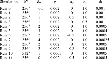
To test the hypothesis that the Elsasser energies and correlation lengths of (unforced) MHD turbulence evolve according to von Kármán–Howarth similarity decay laws – (2.16)–(2.17) and their ‘minus’ partners – and which also requires that the ratio of the parallel and perpendicular characteristic lengths does not change in time, we carry out a set of incompressible MHD simulations with a mean magnetic field,
 $B_{0}\hat{\boldsymbol{z}}$
.
All runs are initialized with kinetic and magnetic spectra proportional to
 $1/[1+(k/k_{0})^{11/3}]$
, with
 $k_{0}=4$
and only the Fourier modes within the band
 $1\leqslant k\leqslant 15$
excited. The initial total energy is always normalized to one. Correlation lengths are small compared to the total box length for all runs. Table 1 contains a summary of the simulation parameters used for this study. Although we are here mainly concerned with anisotropy induced by a mean magnetic field, for context we also include results from an isotropic simulation that lacks a global mean field (run 11).
Simulation parameters for spectral simulations: grid size
 $N^{3}$
, the mean magnetic field strength
 $B_{0}$
, viscosity
 $\unicode[STIX]{x1D708}$
, initial normalized cross-helicity
 $\unicode[STIX]{x1D70E}_{c}=2H_{c}/E$
, initial Alfvén ratio
 $r_{A}=E_{v}/E_{b}$
, time step
 $\text{d}t$
.

We numerically solve (2.1) in a periodic box using a pseudo-spectral solver without any external forcing. All the variables are expanded in a Fourier basis with transfer between real space and Fourier space performed using a fast Fourier transform. We use the second-order Runge–Kutta scheme for time-stepping, and the
 $2/3$
rule for dealiasing. To ensure accuracy of the dissipation rates and spectra we require that
 $k_{max}\unicode[STIX]{x1D701}>1$
for all simulations (Donzis, Yeung & Sreenivasan Reference Donzis, Yeung and Sreenivasan2008; Wan et al.
Reference Wan, Oughton, Servidio and Matthaeus2010). Here
 $k_{max}$
is the maximum resolved wavenumber and
 $\unicode[STIX]{x1D701}$
is the Kolmogorov dissipation length scale.
For strong mean field, the simulations can be performed in non-cubic boxes, provided the parallel cascade (in addition to the perpendicular cascade) is well resolved (Oughton, Dmitruk & Matthaeus Reference Oughton, Dmitruk and Matthaeus2004). For a well-resolved case, a non-cubic simulation domain is not expected to modify the dynamics in incompressible MHD (Bigot et al. Reference Bigot, Galtier and Politano2008b ). We employ a cubic periodic box for all runs discussed herein.
4 Results
To study the decay dynamics of the energy-containing eddies we compute, at each time step, the ‘Elsasser energies’
 $Z_{+}^{2}$
and
 $Z_{-}^{2}$
and their characteristic lengths along each Cartesian coordinate direction. The latter are calculated from the two-point correlation functions (see (2.2)) as
 $$\begin{eqnarray}L_{x}^{\pm }=\frac{1}{Z_{\pm }^{2}}\int _{0}^{\infty }\unicode[STIX]{x1D619}^{\pm }(r,0,0)\,\text{d}r,\end{eqnarray}$$
and similarly for the
 $y$
and
 $z$
components. Here,
 $\unicode[STIX]{x1D619}^{\pm }=\unicode[STIX]{x1D619}_{ii}^{\pm }$
are the trace of the correlation tensors. In Fourier space, we can equivalently define the length scales as
 $$\begin{eqnarray}L_{x}^{\pm }=\frac{\unicode[STIX]{x03C0}}{Z_{\pm }^{2}}\mathop{\sum }_{k_{y},k_{z}}|\boldsymbol{z}^{\pm }(k_{x}=0,k_{y},k_{z})|^{2}.\end{eqnarray}$$
So, the length scales
 $(L_{x}^{\pm })$
are proportional to the reduced spectrum evaluated at zero wavenumber:
 $E_{x}^{red}(k_{x}=0)$
. We define
 $$\begin{eqnarray}\displaystyle & \displaystyle L_{\Vert }^{\pm }=L_{z}^{\pm }, & \displaystyle\end{eqnarray}$$
 $$\begin{eqnarray}\displaystyle & \displaystyle L_{\bot }^{\pm }=\sqrt{\frac{(L_{x}^{\pm })^{2}+(L_{y}^{\pm })^{2}}{2}}. & \displaystyle\end{eqnarray}$$
The factor of
 $1/2$
in the definition of
 $L_{\bot }^{\pm }$
is used because there are two independent components in the perpendicular plane (e.g., Oughton & Matthaeus Reference Oughton and Matthaeus2005). With this definition we usefully have
 $L_{\bot }\approx L_{\Vert }$
for the isotropic case, when
 $L_{x}\approx L_{y}\approx L_{z}$
.
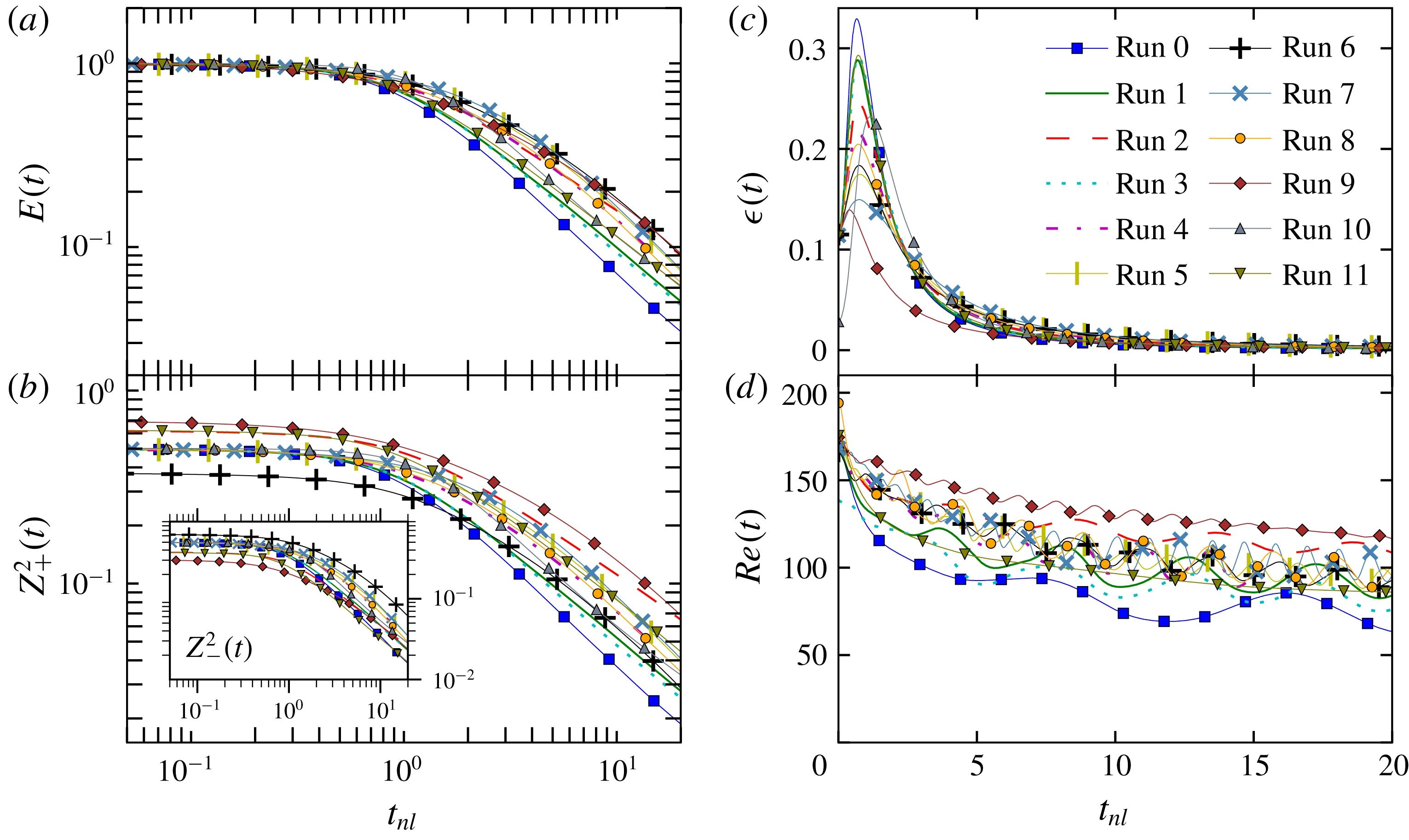
Time history of (a) the total fluctuation energy
 $E$
, (b) the Elsasser energies
 $Z_{\pm }^{2}$
with ‘
 $-$
’ variables shown in the inset, (c) the mean energy dissipation rate
 $\unicode[STIX]{x1D716}=\unicode[STIX]{x1D708}\langle j^{2}+\unicode[STIX]{x1D714}^{2}\rangle$
, and (d) fluid Reynolds number
 $Re$
for the runs listed in table 1. All quantities are defined in the text.

Figure 1 shows the time histories of the total fluctuation energy
 $E$
(magnetic
 $+$
kinetic), Elsasser energies
 $Z_{\pm }^{2}$
, mean energy dissipation rate
 $\unicode[STIX]{x1D716}=\unicode[STIX]{x1D708}\langle j^{2}+\unicode[STIX]{x1D714}^{2}\rangle$
and fluid Reynolds number
 $Re$
for all the runs in table 1. Note that these quantities are associated with the fluctuations and, in particular, the calculation of Elsasser variables, their energies, and the total fluctuation energy does not include the contribution from the mean magnetic field,
 $\boldsymbol{B}_{0}$
. Here,
 $\unicode[STIX]{x1D74E}=\unicode[STIX]{x1D735}\times \boldsymbol{v}$
is the vorticity and
 $\boldsymbol{j}=\unicode[STIX]{x1D735}\times \boldsymbol{b}$
is the current density. The time axis is plotted in units of the initial nonlinear time or ‘eddy turnover’ time,
 $t_{nl}=t/\unicode[STIX]{x1D70F}_{nl}$
. We employ the following definition for the initial eddy turnover time
 $$\begin{eqnarray}\unicode[STIX]{x1D70F}_{nl}=\frac{[L^{+}(0)+L^{-}(0)]/2}{\sqrt{Z_{+}^{2}(0)+Z_{-}^{2}(0)}},\end{eqnarray}$$
where
 $L^{\pm }(0)$
are the initial correlation lengths, and
 $$\begin{eqnarray}L^{\pm }(t)=\frac{\unicode[STIX]{x03C0}}{Z_{\pm }^{2}(t)}\mathop{\sum }_{\boldsymbol{k}}\frac{|\boldsymbol{z}^{\pm }(\boldsymbol{k},t)|^{2}}{|\boldsymbol{k}|}.\end{eqnarray}$$
These are straightforward MHD generalisations of the classical definition of the correlation length or integral scale (Batchelor Reference Batchelor1953; Linkmann et al. Reference Linkmann, Berera, McComb and McKay2015; Bandyopadhyay et al. Reference Bandyopadhyay, Oughton, Wan, Matthaeus, Chhiber and Parashar2018b )
 $$\begin{eqnarray}L_{int}=\frac{\unicode[STIX]{x03C0}}{E^{v}}\mathop{\sum }_{\boldsymbol{k}}\frac{E^{v}(\boldsymbol{k})}{|\boldsymbol{k}|}.\end{eqnarray}$$
Note that we do not recover the directional length scales of (4.1), (4.2) by simply replacing
 $\boldsymbol{k}$
with
 $k_{x}$
in (4.6). The fluid Reynolds number is defined as
 $Re=v^{\prime }L_{int}/\unicode[STIX]{x1D708}$
, where
 $v^{\prime }$
denotes the (average) component root mean square speed with
 $E^{v}=3(v^{\prime })^{2}/2$
. Here,
 $E^{v}(\boldsymbol{k})$
is the modal kinetic energy spectrum and
 $E^{v}$
is the total kinetic energy.
Panels (a) and (b) of figure 1 indicate that, for all runs considered, a power law (in time) is a reasonable approximation to the decay of both the total fluctuation energy and the Elsasser energies, after a few nonlinear times. This behaviour is expected for von Kármán–Howarth similarity decay (Matthaeus et al.
Reference Matthaeus, Zank and Oughton1996). Not all runs have the identical power-law slope and a full explanation for these slight differences is yet to be obtained. However, it is clear that the decay is (approximately) self-similar at these later times. During these
 $t\gtrsim 5\unicode[STIX]{x1D70F}_{nl}$
periods the dissipation rates are much smaller than the peak values but are also only slowly decreasing; the Reynolds numbers are also slowly decreasing (with oscillations).
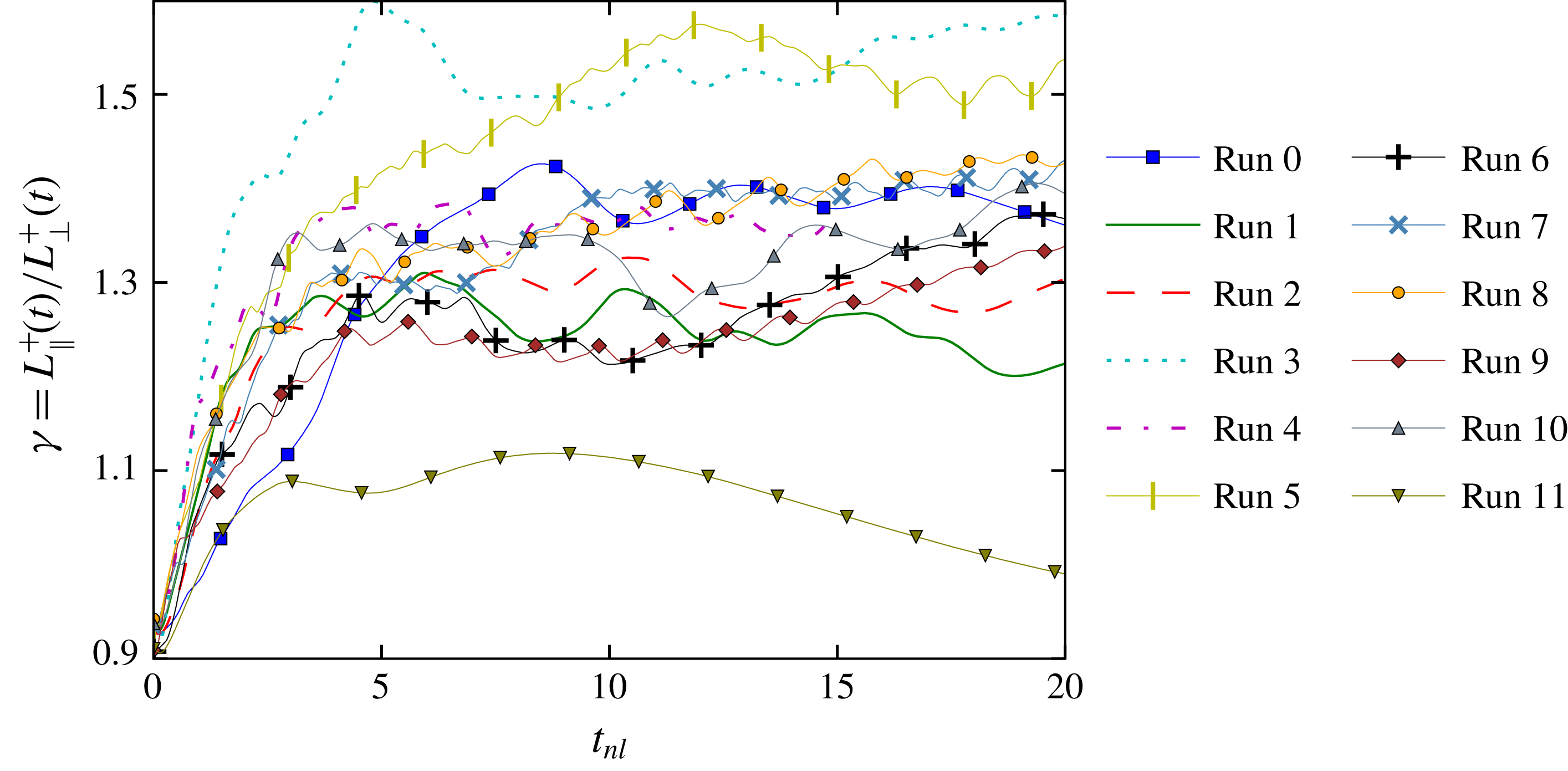
Time evolution of the ratio of parallel to perpendicular correlation lengths,
 $\unicode[STIX]{x1D6FE}=L_{\Vert }^{+}/L_{\bot }^{+}$
, for the runs of table 1.

Figure 2 illustrates the time history of the ratio of the parallel to perpendicular length scales
 $\unicode[STIX]{x1D6FE}=L_{\Vert }^{+}/L_{\bot }^{+}$
, corresponding to the ‘
 $+$
’ Elsasser variable. It is evident that after an initial transient period, the ratio of the two length scales typically saturates to an approximately steady value, with fluctuations around those values.
A closer inspection of figures 1 and 2 reveals that the dissipation rate reaches its maximum near unit nonlinear time. However,
 $\unicode[STIX]{x1D6FE}$
values saturate at a somewhat later time
 $t_{nl}\sim 2{-}5$
. This behaviour can probably be explained by noting that modifying the very large length scales takes a long time. The correlation lengths may become steady after the lowest wavenumber part of the spectrum is well populated. Since dissipation involves high wavenumber regions of the spectrum, where the characteristic time scales are much faster than those of the energy-containing eddies, it is perhaps not surprising that the dissipation rate peaks before
 $\unicode[STIX]{x1D6FE}$
saturates.
Although
 $\unicode[STIX]{x1D6FE}$
attains different values for different simulation sets, figure 2 indicates that for all cases
 $\unicode[STIX]{x1D6FE}$
remains approximately stationary for many nonlinear times. Furthermore, for the non-zero mean-field cases,
 $L_{\Vert }^{+}$
is always greater than
 $L_{\bot }^{+}$
, indicating that the correlation lengths along the mean-field are longer than those perpendicular to it, due to the cascade preferentially transferring energy in the perpendicular directions (Shebalin et al.
Reference Shebalin, Matthaeus and Montgomery1983; Grappin Reference Grappin1986; Matthaeus, Goldstein & Roberts Reference Matthaeus, Goldstein and Roberts1990; Oughton et al.
Reference Oughton, Priest and Matthaeus1994; Goldreich & Sridhar Reference Goldreich and Sridhar1995; Teaca et al.
Reference Teaca, Verma, Knaepen and Carati2009).
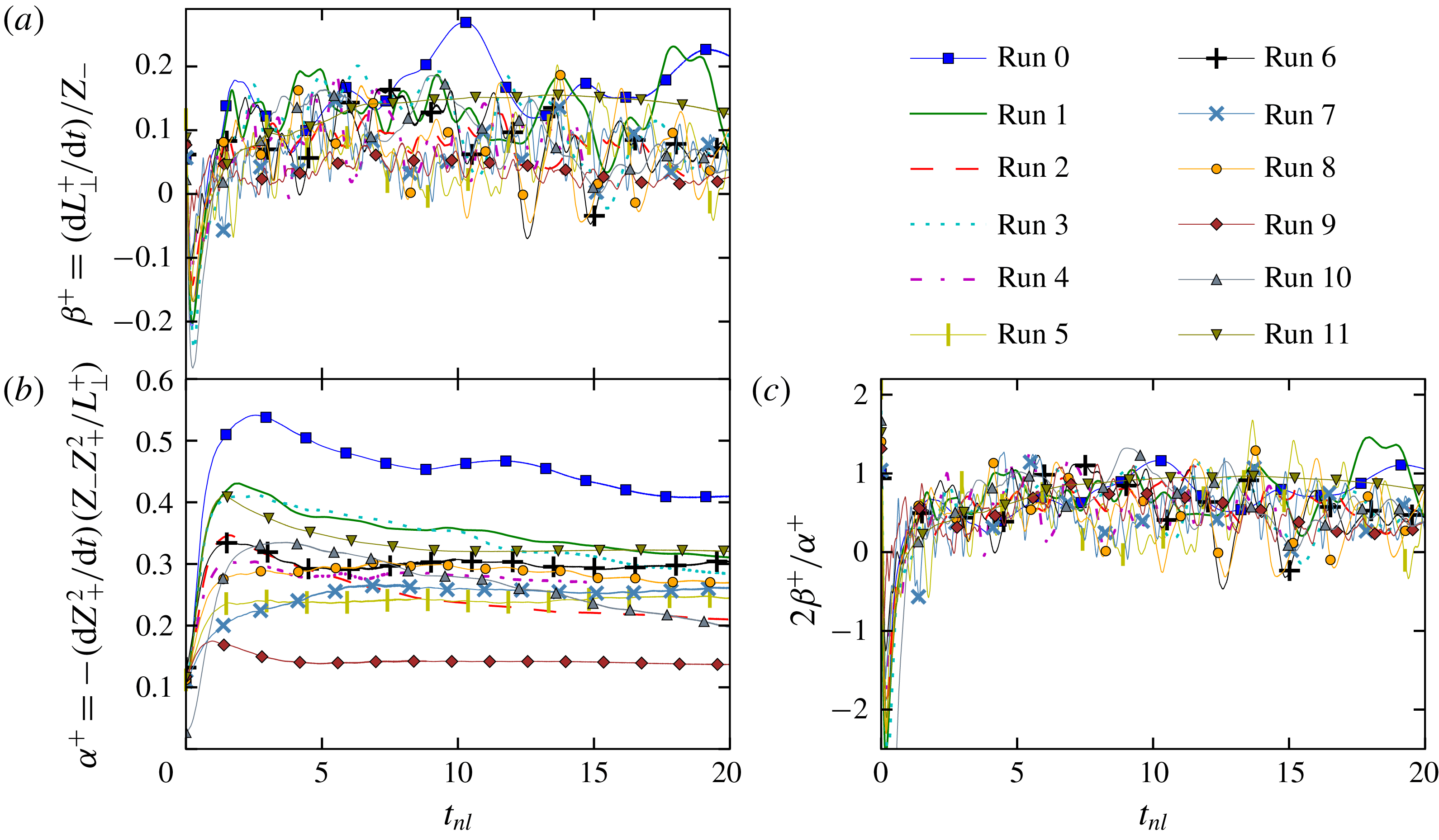
Time evolution of the two von Kármán constants: (a)
 $\unicode[STIX]{x1D6FD}^{+}=(\text{d}L_{\bot }^{+}/\text{d}t)/Z_{-}$
. (b)
 $\unicode[STIX]{x1D6FC}^{+}=-(\text{d}Z_{+}^{2}/\text{d}t)(Z_{-}Z_{+}^{2}/L_{\bot }^{+})$
, and (c) twice the ratio of the two constants,
 $2\unicode[STIX]{x1D6FD}^{+}/\unicode[STIX]{x1D6FC}^{+}$
, associated with the family of conservation laws, equation (2.18).

Figure 2 contains the main results of this paper. (Plots for
 $\unicode[STIX]{x1D6FE}^{-}=L_{\Vert }^{-}/L_{\bot }^{-}$
, not shown, are completely analogous.) Having established that the ratio of parallel to perpendicular length scales remain (roughly) constant in time, we proceed to examine whether the proposed von Kármán similarity decay is satisfied for MHD fluids in the presence of a global magnetic field. In figure 3, we show the two ‘von Kármán constants’
 $\unicode[STIX]{x1D6FC}^{+}$
and
 $\unicode[STIX]{x1D6FD}^{+}$
, corresponding to the ‘
 $+$
’ Elsasser variables, as functions of time. If the similarity decay hypothesis is indeed satisfied, these two quantities should maintain constant values in time. Figure 3(a) shows the rate of change of perpendicular length scale
 $L_{\bot }^{+}$
normalized to
 $Z_{-}$
, which, if the decay obeys a similarity solution is a constant,
 $\unicode[STIX]{x1D6FD}^{+}$
. Panel (b) plots the (negative) normalized rate of change of
 $Z_{+}^{2}$
as a function of time; again, if the decay obeys a similarity this will be a constant,
 $\unicode[STIX]{x1D6FC}^{+}$
. A central difference scheme is used to evaluate the time derivatives. It is clear from the two panels of figure 3 that the similarity decay hypothesis, as proposed in Wan et al. (Reference Wan, Oughton, Servidio and Matthaeus2012), is well supported by the simulation results presented here.
Recall also, from (2.18), that the conserved quantity associated with the self-similar decay depends on the ratio
 $2\unicode[STIX]{x1D6FD}^{+}/\unicode[STIX]{x1D6FC}^{+}$
. This ratio is displayed in panel (c) of figure 3 where it can be seen that it attains a steady-state value of somewhat less than unity, after an initial adjustment phase. From Dryden (Reference Dryden1943) and von Kármán & Lin (Reference von Kármán and Lin1949) self-similar decay for all scales requires
 $\unicode[STIX]{x1D6FC}^{\pm }=\unicode[STIX]{x1D6FD}^{\pm }$
. This situation corresponds to the case of decay with constant turbulent viscosity,
 $Z^{\pm }L^{\pm }=\text{const}.$
, or equivalently decay at constant Reynolds number. Clearly, this is not satisfied rigorously in the simulations presented here. Further, the plotted values of
 $2\unicode[STIX]{x1D6FD}^{+}/\unicode[STIX]{x1D6FC}^{+}$
appear to eliminate the possibility of similarity decay with
 $(Z^{\pm })^{2}L^{\pm }=\text{const}.$
, physically corresponding to the case of constant area under the correlation function. Although only the ‘
 $+$
’ Elsasser variables are shown here, the results are similar for the ‘
 $-$
’ Elsasser variables. As an aside we note that applications of MHD decay phenomenologies within studies of the transport of solar wind fluctuations (e.g., Matthaeus et al. (Reference Matthaeus, Zank and Oughton1996), Zank, Matthaeus & Smith (Reference Zank, Matthaeus and Smith1996), and many subsequent papers) have previously employed both the
 $\unicode[STIX]{x1D6FD}/\unicode[STIX]{x1D6FC}=1$
and the
 $2\unicode[STIX]{x1D6FD}/\unicode[STIX]{x1D6FC}=1$
conditions.
Next, we briefly discuss the effect of anisotropy due to the mean magnetic field strength
 $B_{0}$
and/or the cross-helicity strength. Of particular interest here is the variation of
 $\unicode[STIX]{x1D6FE}=L_{\Vert }^{+}/L_{\bot }^{+}$
with
 $B_{0}$
and with the magnitude of the initial normalized cross-helicity
 $\unicode[STIX]{x1D70E}_{c}$
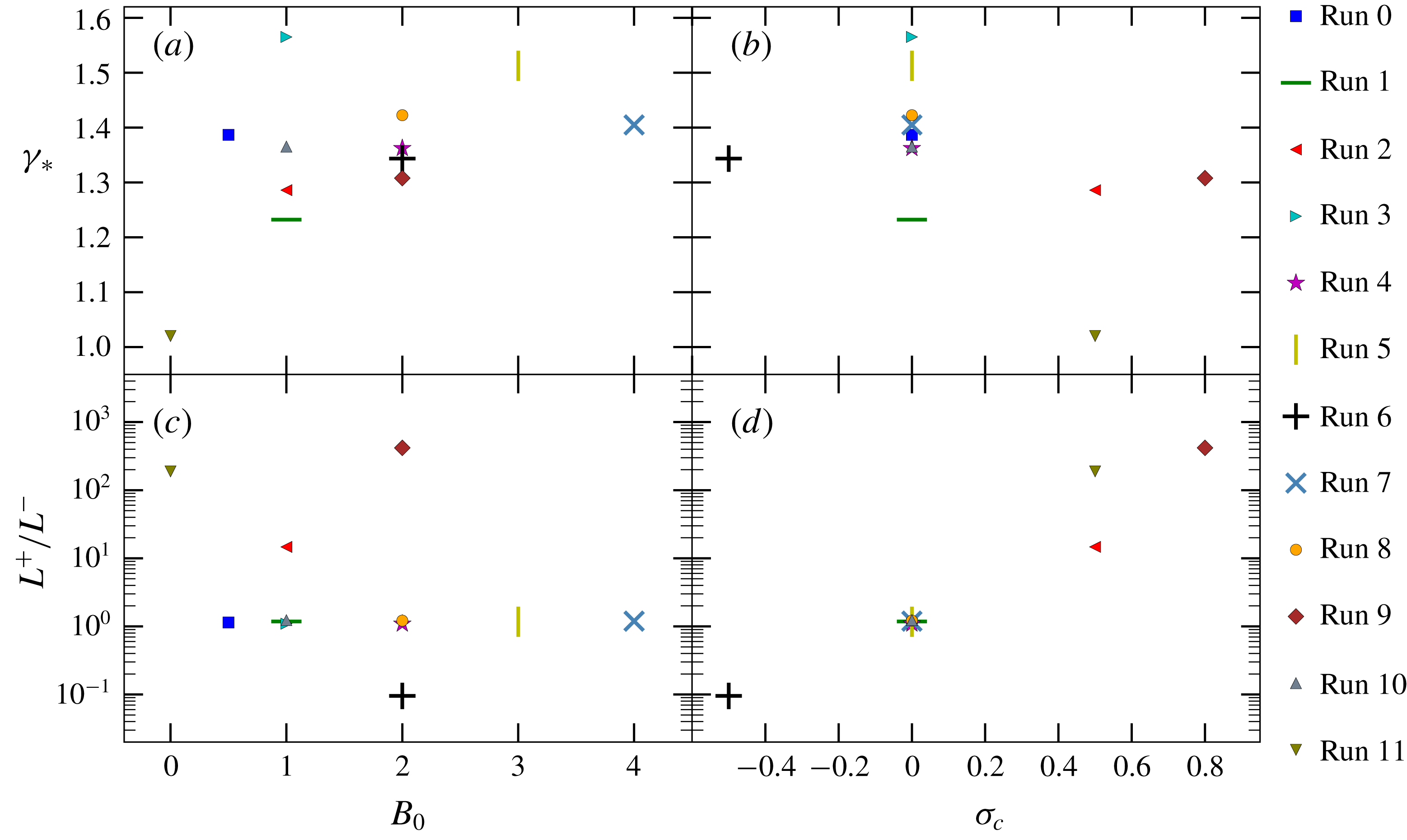
. Figure 4 shows the asymptotic values of
 $\unicode[STIX]{x1D6FE}$
for all the runs. These asymptotic values, denoted
 $\unicode[STIX]{x1D6FE}_{\ast }$
, are obtained by averaging
 $\unicode[STIX]{x1D6FE}$
over the final five nonlinear times for each run. Within the limited parameter range scan of
 $B_{0}$
and
 $\unicode[STIX]{x1D70E}_{c}$
covered by the simulations presented here, it appears that
 $\unicode[STIX]{x1D6FE}_{\ast }$
initially increases with
 $B_{0}$
but the effect then saturates for higher values of
 $B_{0}$
. This behaviour is expected since the mean-field-induced anisotropy renders the system approximately two-dimensional; i.e.,
 $L_{\Vert }>L_{\bot }$
. On the other hand, from panel (b) of figure 4, no clear scaling can be deduced between
 $\unicode[STIX]{x1D6FE}_{\ast }$
and
 $\unicode[STIX]{x1D70E}_{c}$
.
Variation of the asymptotic values of
 $\unicode[STIX]{x1D6FE}=L_{\Vert }^{+}/L_{\bot }^{+}$
with (a) mean-magnetic-field strength
 $B_{0}$
and (b) the normalized cross-helicity
 $\unicode[STIX]{x1D70E}_{c}$
, for the runs of table 1. Panels (c) and (d) plot the variation of the ratio
 $L^{+}/L^{-}$
with
 $B_{0}$
and
 $\unicode[STIX]{x1D70E}_{c}$
, respectively.

A related quantity of interest is the ratio of the length scales corresponding to the ‘
 $+$
’ and ‘
 $-$
’ Elsasser variables. Figure 4(c,d) illustrate the variation of the ratio
 $L^{+}/L^{-}$
. Again, the reported values are the temporal averages over the final five nonlinear time units. Here, we see that there is no evident scaling with the mean-field strength
 $B_{0}$
. However, panel (d) exhibits a rough increasing scaling of
 $L^{+}/L^{-}$
with
 $\unicode[STIX]{x1D70E}_{c}$
. This result is consistent with the explanation provided by Matthaeus, Goldstein & Montgomery (Reference Matthaeus, Goldstein and Montgomery1983) and Ghosh, Matthaeus & Montgomery (Reference Ghosh, Matthaeus and Montgomery1988), who argue that for high cross-helicity (say, positive), one of the Elsasser fields
 $(\boldsymbol{z}_{-})$
is weak and it is almost passively advected towards high wavenumber by the dominant Elsasser field
 $(\boldsymbol{z}_{+})$
. This kind of tendency would result in dissimilar values of the two Elsasser field length scales
 $(L^{+}\gg L^{-})$
. From figure 4, the zero cross-helicity runs, run 0, 1, 3, 4, 5, 7, 8, 10, maintain
 $L^{+}/L^{-}\approx 1$
. The positive cross-helicity runs, run 2, 9, 11, show
 $L^{+}/L^{-}>1$
, with increasing value of
 $L^{+}/L^{-}$
as
 $\unicode[STIX]{x1D70E}_{c}$
increases. Run 6 has
 $\unicode[STIX]{x1D70E}_{c}<0$
and consequently
 $L^{+}/L^{-}<1$
for this case.
5 Discussion
We have examined the validity of a von Kármán–Howarth-like similarity decay phase in anisotropic 3-D MHD in the presence of an externally supported mean magnetic field (
 $\boldsymbol{B}_{0}$
), as derived in Wan et al. (Reference Wan, Oughton, Servidio and Matthaeus2012). An analytic result is that a similarity decay phase is only followed in an MHD fluid (with a
 $\boldsymbol{B}_{0}$
) if the ratio of the parallel to perpendicular characteristic length scales,
 $\unicode[STIX]{x1D6FE}=L_{\Vert }^{+}/L_{\bot }^{+}$
, remains constant in time. Using numerical simulations, performed with a range of different parameters, we find that the ratio of parallel to perpendicular length scales does indeed maintain an approximately steady value during the decay of the MHD turbulence, after an initial build-up phase. This result provides substantial support for the occurrence of similarity decay of energy in MHD turbulence with a mean-field.
Additionally, since the ratio of the parallel and perpendicular length scales maintains a constant value this implies that only one of the length scales evolves independently. This has useful consequences for global turbulence-based modelling of the solar wind and other astrophysical plasmas. Often in such models a von Kármán-like phenomenology is invoked (e.g., Breech et al. Reference Breech, Matthaeus, Minnie, Bieber, Oughton, Smith and Isenberg2008; Oughton et al. Reference Oughton, Matthaeus, Smith, Breech and Isenberg2011; Usmanov, Goldstein & Matthaeus Reference Usmanov, Goldstein and Matthaeus2014). If the parallel and perpendicular lengths maintain a constant proportion in the solar wind, it may be sufficient to evolve the length scale along only one direction, simplifying the calculations and possibly making the computations less expensive.
The results presented in this paper are important for understanding heating and acceleration of space plasmas such as the solar corona, solar wind and magnetospheric plasmas. The conclusions should also be useful for understanding and modelling the role of turbulence in the evolution and dynamics of astrophysical plasmas and laboratory plasmas.
We note that although the runs have the same initial conditions, after a few nonlinear times they evolve independently to distinct states. Therefore, we suggest that the result, that
 $L_{\Vert }/L_{\bot }$
maintains a steady value, does not depend on the large-scale eddies being of the same form in the parallel and perpendicular directions.
The applicability of the theory for modest Reynolds number warrants some discussion. To arrive at (2.16) and (2.17), we neglect the two terms proportional to
 $\unicode[STIX]{x1D708}$
in (2.14). This step can be justified by a simple calculation to estimate the order of magnitude of the neglected terms compared to the retained terms in (2.14). Let us compare the two terms
 $\{\text{d}Z_{+}^{2}/\text{d}t\}[f]$
and
 $\{2\unicode[STIX]{x1D708}Z_{+}^{2}/{L_{\Vert }^{+}}^{2}\}[\unicode[STIX]{x2202}^{2}f/\unicode[STIX]{x2202}\unicode[STIX]{x1D702}_{\Vert }^{2}]$
. For simplicity, we ignore the notations
 $\Vert$
,
 $\bot$
,
 $\pm$
, etc., and assume
 $f\sim \exp (-\unicode[STIX]{x1D702})$
. Then, we can compare the two terms as
 $$\begin{eqnarray}\frac{\text{d}Z^{2}}{\text{d}t}:\unicode[STIX]{x1D708}\frac{Z^{2}}{L^{2}}.\end{eqnarray}$$
For a consistency check, if we insert the desired solution,
 $\text{d}Z^{2}/\text{d}t\sim Z^{3}/L$
, on the left-hand side we obtain
 $$\begin{eqnarray}\frac{Z^{3}}{L}:\unicode[STIX]{x1D708}\frac{Z^{2}}{L^{2}}.\end{eqnarray}$$
Noting that
 $ZL/\unicode[STIX]{x1D708}\sim Re$
this yields
 $$\begin{eqnarray}1:\frac{1}{Re}.\end{eqnarray}$$
So, from this very crude argument, the theory is expected to hold for
 $Re\gg 1$
. In practice, one finds that the conditions for a similarity decay law are much less stringent than, say, the conditions for the Kolmogorov
 $-5/3$
slope (von Kármán & Lin Reference von Kármán and Lin1949). In the simulations shown here, the lowest value of Reynolds number is around 50,
 $Re\sim 50$
. Therefore, in the worst case scenario, the neglected terms are approximately
 $50$
times smaller than the retained terms in (2.14). It is clear from the results that this level of smallness for the terms proportional to
 $\unicode[STIX]{x1D708}$
is sufficient to satisfy an approximate similarity decay.
However, we can infer the effect of Reynolds number and large-scale eddy strength
 $({\sim}ZL)$
by examining results from two simulations, run 3 and run 10. These differ only by Reynolds number with run 10 having the larger
 $Re$
. From figure 4, run 3 has a higher value of
 $\unicode[STIX]{x1D6FE}^{\ast }$
(i.e., asymptotic
 $L_{\Vert }^{+}/L_{\bot }^{+}$
). One factor contributing to the different values of
 $\unicode[STIX]{x1D6FE}^{\ast }$
is probably the different grid size in the two simulations. Further, it is known that mean-field-induced anisotropy depends on Reynolds number, so that may play a role here. The ratio
 $L^{+}/L^{-}$
, on the other hand, admits almost equal values for the two runs, presumably since the cross-helicity is the same for both cases. The ‘energy’ similarity decay constant,
 $\unicode[STIX]{x1D6FC}^{+}$
, as expected, decreases from run 3 to run 10, due to increased
 $Re$
(Linkmann et al.
Reference Linkmann, Berera, McComb and McKay2015, Reference Linkmann, Berera and Goldstraw2017; Bandyopadhyay et al.
Reference Bandyopadhyay, Oughton, Wan, Matthaeus, Chhiber and Parashar2018b
). However, the ‘length scale’ similarity constant,
 $\unicode[STIX]{x1D6FD}^{+}$
, appears to be less sensitive to Reynolds number.
It is interesting to note that Kármán–Howarth-like similarity decay has been observed in two-dimensional (2-D) MHD (Biskamp & Schwarz Reference Biskamp and Schwarz2001). However, a comparison of similarity solutions in 2-D MHD (or two-and-a-half-dimensional, that is, three-component vectors in a two-dimensional plane (2.5-D MHD)) and strong-mean-field 3-D MHD is not entirely straightforward since 2-D MHD also admits an inverse cascade of mean-squared magnetic potential,
 $A$
. This requires that some magnetic energy is also inverse cascaded and is thus not available for direct cascade to the dissipative small scales. Exploring that parameter space is beyond the scope of the current paper. In particular, the 2-D runs would need to scan
 $E/A$
(
 $E$
is the energy) and the 3-D ‘comparison’ runs would require a scan of
 $B_{0}$
, as well as varying the initial polarization (2-D versus ‘2.5-D’).
Further, using 2.5-D fully kinetic particle-in-cell simulations, it has been shown that weakly collisional plasmas support similarity decay (Wu et al.
Reference Wu, Wan, Matthaeus, Shay and Swisdak2013; Parashar et al.
Reference Parashar, Matthaeus, Shay and Wan2015). It will be interesting to extend and test the similarity decay phenomenologies discussed here to three-dimensional kinetic simulations, shear driven flows, compressible plasmas, etc. It is not clear why the quantity
 $\unicode[STIX]{x1D6FE}=L_{\Vert }/L_{\bot }$
attains a constant value. Other types of turbulent flow that develop anisotropy, due to rotation, stratification, convection, etc., may also admit a similar stabilization of the ratio of the parallel and perpendicular length scales. Another interesting direction in which the similarity solution can be extended is quasi-static MHD turbulence (see Verma (Reference Verma2017) for a review). We plan to take up these endeavours in the future.
Acknowledgements
This research is supported by NASA under grant NNX17AB79G, and Heliospheric Supporting Research grants 80NSSC18K1210 and 80NSSC18K1648, as well as the Parker Solar Probe Project under Princeton subcontract SUB000016S. The simulations were performed using the Dante and Casella clusters at the University of Delaware, USA.