Joint communication and computation

In a classical scenario of telecommunication network as depicted in Figure 1, different datasets collected by the sensors from distributed locations are transmitted through wireless channels to servers for computing. In this structure, the sensors are transmitter side (TX), and the servers are receiver side (RX). The major nonlinearity in TX is a PA, and in the RX is a low noise amplifier (LNA). There can be multiple UEs in the network. The communication task and the computation task are implemented separately.

Figure 1.

A classical scheme with separated communication and computation tasks: data collected by sensors are sent through the telecommunication network to server for computing.

The scheme of J2C network introduced in [Reference Wang, Özçelikkale and Benlarbi-Delai15] integrates the communication and computation into a single implementation, which reduces the total cost and latency. As illustrated in Figure 2, the telecommunication network is turned into a wireless NN where the nonlinearity of the PA and LNA is considered as activation functions of a neuron. The neurons upstream of the synapse are denoted as “pre-neuron” and those downstream of the synapse are denoted as “post-neuron.” The synapse of a classical NN is linear, which is realized by the wireless channel with a complex gain and phase delay as the weight $w$. A multi-path channel can be expressed as:

(1)\begin{equation} y_{RX}(n)=\sum_{m=0}^{M}\sum_{p=1}^{P_m} a_{m} h_{m,p} y_m(n-l_{m,p}) +z(n), \end{equation}

Figure 2.

Structure of a wireless neural network.

where $M$ is the number of connected pre-neurons, $y_m$ is the output of the $m$-th pre-neuron, $y_{RX}$ is the signal received by the RX, $z(n)$ denotes the channel noise, $a_{m}$ are adjustable and correspond to PA settings, $P_m$ is the total number of paths in the $m$-th channel, $h_{m,p}$ are beamed channel coefficients, $l_{m,p}$ are the delay of the $p$-th path for the $m$-th channel. In case of line-of-sight (LOS) channel, we have $P_m$=1. If we define the synapse weight as $w_{m} =a_{m} h_{m,p}$, the optimal value of $w_{m}$ after training can be configured by modifying $a_{m}$ through PA gain control and $h_{m,p}$ through beam control. One way to control the channel gains $h_{m,p}$ is through the direction of beams [Reference Mavridis, Sarrazin, Petrillo, De Doncker and Benlarbi-Delaï22].

In case that an array of identical PAs is deployed at TX upstream of the antenna array for beam-forming, the nonlinear behavior of the sum of the PA array is similar to a single PA. For simplicity, we consider only a single PA per TX. The datasets are generated from sensors on the edge of the network and are distorted by these “activation functions” when being transmitted to the other side of the network. The computation of the input data is processed in the J2C network through the transmission within the communication network.

The MNIST dataset is used to test the computational capacity of this J2C network. The MNIST contains a set of pictures with handwriting numbers from 0 to 9. The network for image recognition task is fed with the pixels at the input and is expected to predict the correct number at the output.

In the classical scheme, the data are correctly transmitted through network thanks to different modulation/demodulation and linearization techniques, and then are processed with a ReLU-based NN at the receiver. The performance of ReLU-based NN is given in Table 1.

Table 1.

Accuracy of an NN with 1 hidden layer based on PA model with and without memory effects

In the study of [Reference Wang, Özçelikkale and Benlarbi-Delai15], the simulation of the J2C network utilizes a memoryless PA model proposed by Saleh et al. in [Reference Saleh23] as the nonlinear activation functions of neurons:

(2)\begin{equation} y(n)=\frac{\alpha_Ax(n)}{1 + \beta_Ax(n)^2} \end{equation}

where $x(n)$ is the input signal of the model, $\alpha_A$ and $\beta_A$ are constants. In the study of PA behavioral modeling, the nonlinearity and memory effects are two main factors to be considered. A real-valued PA model based on Volterra series to mimic its behavior in RF domain is discussed in [Reference Wang, Hou and Eriksson24]. If we decompose the nonlinearity of (2) with Taylor expansion or analyze the Volterra series-based model, we can see as in Figure 3 that the $k$-th order nonlinearity occupies $k$ times of the bandwidth of PA input signal.

Figure 3.

Bandwidth expansion due to nonlinearity.

Usually, a band-pass filter is applied after the PA to ensure the output signal remains within a designated frequency range. This filter will have an impact on the activation function when the bandwidth of PA input signal is large so that the out-of-band distortion locates outside the designated frequency range. Along with the enlargement of PA input signal, the memory effects of the PA also become inevitable for consideration. Therefore, the Saleh model (2) works well only in case that the PA input signals are modulated in very narrow bandwidth.

Considering that the behavior of the PA can vary due to environmental temperature fluctuations and its own thermal effects, which effectively introduce noise into its characteristics, we evaluate the computing performance by adding Gaussian random noise to the PA model parameters, $\alpha_A$ and $\beta_A$, with a standard deviation corresponding to 50% of their nominal values. Since all PAs in the network are assumed to operate under similar conditions, we apply this perturbation synchronously across all units. As shown in Table 1, the network is sufficiently robust against these disturbances.

More studies on the neuronal properties of the PA are needed for the case that the bandwidth of input signal is large. In this paper, we examine the pHEMT PA by cascading a filter with memory depth $L$=6 in its modeling. The results in Table 1 show that the accuracy is significantly reduced when the number of neurons is around 8. However, when the number of neurons is over 20, the memory effects of the PA has negligible impact on the performance of J2C network computing .

If we denote the complexity of multiplication, addition, softmax, modulation, demodulation, predistortion, coding, and postdistortion by $C_{\times}$, $C_{+}$, $C_{\text{mod}}$, $C_{\text{dem}}$, $C_{\text{pre}}$, $C_{\text{cod}}$, and $C_{\text{post}}$, respectively, the classical network needs a computational complexity of

(3)\begin{equation} \begin{split} &C_{\text{com}}+(N_{\text{input}}N_{\text{hidden}}+N_{\text{hidden}}N_{\text{output}})C_{\times} \\ +&(N_{\text{hidden}}+N_{\text{output}})(C_{+}+C_{\text{relu}})+N_{\text{output}}C_{\text{softmax}} \end{split} \end{equation}

where the communication cost is $C_{\text{com}}=C_{\text{mod}}+C_{\text{dem}}+C_{\text{pre}}+C_{\text{cod}}+C_{\text{post}}$, number of neurons in the input, hidden, and output layers are denoted by $N_{\text{input}}$, $N_{\text{hidden}}$, and $N_{\text{input}}$, respectively. If we consider the multiplications of weights with output of each neuron are in parallel and have the same computing time, the latency of the classical scheme can be expressed as

(4)\begin{equation} \begin{split} T_{\text{com}}+2(T_{+}+T_{\times})+T_{\text{relu}}+T_{\text{softmax}} \end{split} \end{equation}

where the communication latency is $T_{\text{com}}=T_{\text{mod}}+T_{\text{dem}}+T_{\text{pre}}+T_{\text{cod}}+T_{\text{post}}$, the latency of addition, multiplication, ReLU, and Softmax are denoted as $T_{+}$, $T_{\times}$, $T_{\text{relu}}$, $T_{\text{softmax}}$, respectively.

In the J2C scheme, the modulation/demodulation and linearization techniques are no longer necessary. Only a pre-processing of data to regroup the pixels for inputs of TX and a post-processing of Softmax are needed. The computational complexity is thus reduced to

(5)\begin{equation} \begin{split} (N_{\text{input}}N_{\text{hidden}})C_{\times}+N_{\text{output}}C_{\text{softmax}}, \end{split} \end{equation}

and the latency is reduced to

(6)\begin{equation} \begin{split} T_{+}+T_{\times}+T_{\text{softmax}}, \end{split} \end{equation}

since the multiplications and additions between the hidden layer and output layer can be realized by the wireless channel through over-the-air computing technique [Reference Wen, Zhu and Huang25].

To mimic the scenario where the sensors have their own data without sharing, the pixel information is partitioned in [Reference Wang, Özçelikkale and Benlarbi-Delai15] into $N_{\text{hidden}}$ sets, which are fed to $N_{\text{hidden}}$ TX as depicted in Figure 4. These $N_{\text{hidden}}$ TX are connected to 10 RX via wireless channel. With a softmax function at each RX downstream of the LNA, the RX whose index corresponds to the correct handwriting number is indicated. The simulation gives an accuracy $\approx 85\%$ when $N_{\text{hidden}}$ is 14 and $\approx 90\%$ when $N_{\text{hidden}}$ is 56.

Figure 4.

The neural network for MNIST test.

An earlier study related to this paper was presented at EuMW 2024 [Reference Wang, Özçelikkale and Benlarbi-Delai15]. In this section as well as in [Reference Wang, Özçelikkale and Benlarbi-Delai15], we have studied the performance of a PA model as a neuron model in a shallow NN, which gives a satisfactory accuracy in handwriting recognition. A study can be made in reverse direction: does a neuron model work well in describing the PA behavior?

Neuromorphic model matching PA behavior

Since the behavior of a real PA can be complicated in different scenarios, a fundamental research on the correlation between measured PA behavior and the most biological plausible model, i.e. HH model, is carried out in this section. To study the neuronal property of a real PA, we first measure its behavior by acquiring its output signal when feeding it a specific input signal, such as a modulated orthogonal frequency-division multiplexing (OFDM) signal. Then, we analyze if this behavior can be described with the HH model by identifying the model parameters. Since the HH model is composed of differential equations, which are not linear-in-parameter, we adopt BE method to address this problem. The statistical probabilities of the identified parameters will be determined.

Dataset collection

In this paper, two different types of PA are used for experimental study. The first PA under test is a HMC994APM5E PA from Analog Devices in the Test bench at GeePs, Sorbonne University, as shown in Figure 5. This is a GaAs pHEMT MMIC wideband PA. Its nominal gain at 28 GHz is 14 dB and the saturated output power is 29 dBm. The supply voltage is 10 V. The stimulus 400 MHz 5G NR signal generated at the baseband in the PC workstation is fed to an Arbitrary Waveform Generator (AWG) at 10 GHz sampling frequency and centered at 1.5 GHz. Upconversion to 28 GHz by a mixer and a band-pass filter of 27-29 GHz are set up in front of the DUT. The AM/AM curve of the PA is shown in Figure 7. Since this study focus on the behavioral modeling, the magnitude and the unit of measured data are not important. For easier implementation of modeling, we normalize the input to 0-1.5 and the output to 0-0.1.

Figure 5.

Test bench for pHEMT PA characterization at GeePs, Sorbonne University.

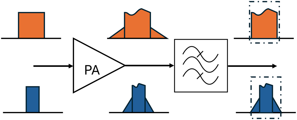
Normally in industrial application, there is another band-pass filter at the PA output to keep its spectrum inside the designated frequency range as illustrated in Fig. 6. In case of wide-band input signal as colored in orange, the out-of-band distortion will be removed before emission through out-of-band DPD [Reference Gilabert, López-Bueno and Montoro26] and filter while the in-band distortion is still kept. The orange dots in Figure 7 show the behavior of PA cascaded with a band-pass filter if the designated frequency range has a bandwidth of 400 MHz. In case of narrow-band input signal as colored in blue, the most part of out-of-band distortion will be kept along with the in-band distortion. The blue dots in Figure 7 show the PA behavior without a filter in case that the designated frequency range is wide enough. We can see that the filtering effect augments the saturated power and brings heavier memory effects, but the nonlinearity shape stays sigmoid.

Figure 6.

The system of PA followed by a band-pass filter.

Figure 7.

AM/AM curves from PA tested with 400 MHz 5G NR signal.

The second PA under test is a three-way Doherty high-PA, as illustrated in Figure 8. It comprises three Ampleon LDMOS BLF7G22LS-130 devices, each featuring a 1dB compression point output power of 57dBm (500W) and a nominal gain of 16dB. Figure 9 shows the measured AM-AM and AM-PM characteristics of this PA when driven with a 20MHz LTE signal centered at 2.14GHz. Under these test conditions, the Doherty PA achieves an average output power of 44 dBm.

Figure 8.

Three-way Doherty PA.

Figure 9.

AMAM & AMPM curves of Doherty PA.

Bio-neuron behavior: Hodgkin–Huxley model

(7)\begin{equation} \begin{cases} \begin{aligned} \frac{d V_m}{dt} &=\frac{1}{C_m}\bigg{[}I_{ext} \ -g_{Na}m^3h(V_m - V_{Na})\\ &\quad - g_{K}n^4(V_m - V_{K}) - g_L(V_m - V_L) \bigg{]} \\ \frac{d m}{dt} &= \alpha_m(V_m)\cdot(1-m) -\beta_m(V_m)\cdot m\\ \frac{d h}{dt} &= \alpha_h(V_m)\cdot(1-h) -\beta_h(V_m)\cdot h \\ \frac{d n}{dt} &= \alpha_n(V_m)\cdot(1-n) -\beta_n(V_m)\cdot n, \end{aligned} \end{cases} \end{equation}

with

(8)\begin{equation} \begin{cases} \begin{aligned} \alpha_m(V_m)&= \frac{-0.1(V_m + 50)}{\operatorname{exp}(-(V_m + 50)/10)-1 } \\ \beta_m(V_m) &= 4 \operatorname{exp} \left( \frac{-(V_m+75)}{18} \right)\\ \alpha_h(V_m)&= 0.07 \operatorname{exp} \left( \frac{-(V_m+75)}{20} \right)\\ \beta_h(V_m) &= \frac{1.0}{\operatorname{exp}(-(V_m + 45)/10)+1 } \\ \alpha_n(V_m)&= \frac{-0.01(V_m + 65)}{\operatorname{exp}(-(V_m + 65)/10)-1 } \\ \beta_n(V_m) &= 0.125 \operatorname{exp} \left( \frac{-(V_m+75)}{80} \right). \end{aligned} \end{cases} \end{equation}

where $V_m$ is the membrane voltage, $C_m$ is the membrane capacitance, $I_{ext}$ is the external current applied; $V_{Na}$, $V_{K}$, and $V_{L}$ are the equilibrium potentials for sodium, potassium, and leakage ions, respectively; $g_{Na}$, $g_{K}$, and $g_{L}$ are the maximum conductance for the channels of sodium, potassium, and leakage ions, respectively. And $m$, $h$, and $n$ are the dimensionless gate variables that characterize the activation and inactivation of sodium and potassium channels. In principle, the HH model presents how the spikes are generated under the effect of $Na$- and $K$- ions passing. The values of $C_m$, $g_{Na}$, $g_{K}$ and $g_{L}$ determines the transfer function of the neuron, i.e. the relation between $I_{ext}$ and the firing rate of $V_m$. While modeling the PA behavior with HH model, we take the input signal as $I^D_{ext}$ and the output signal as the firing rate $F^D$.

We use Python code to perform numerical simulation for the HH model with the parameters’ values of the paper [Reference Pant27]. Figure 10 shows an example of numerical simulation of HH model response with $I_{ext}$=20 $\mu A.\text{cm}^{-2}$ as a function of time.

Figure 10.

Simulation examples of HH model.

Rate coding

As we can see from Figure 10 that $V_m$ bears periodical patterns. A technical question is how to compute the period of $V_m$. In each period, we notice that $V_m$ bears a local minimum, which is a stationary point, such that the derivative with respect to time shall be $0$. Thus, we apply the forward difference to compute the discrete first-order derivative for $V_m$, and we trace the points $t_j$ such that the discrete derivative $dV_m/dt$ is negative at $t_{j-1}$ but positive at $t_j$. The distance between these stationary points $\{t_j\}$ is set to be the period.

The firing rate is the inverse of the calculated period, which will be used in the BE of the parameters.

Using the parameters of [Reference Pant27], we observe that the simulation results have a clear periodic pattern while $I_{ext}$ is in the range $[10,140]$ $\mu A.\text{cm}^{-2}$. And the firing rate is monotonically increasing with respect to $I_{ext}$. To use the data presented in Figure 7 for the parameter estimation of the HH model, we perform linear transformation of the data. We focus on the range $[10,140]$ $\mu A.\text{cm}^{-2}$ of $I_{ext}$, and the simulation results show that the firing rate equals to $0.068299$ kHz when $I_{ext} = 10$ $\mu A.\text{cm}^{-2}$ and $0.16419$ kHz when $I_{ext} = 140$ $\mu A.\text{cm}^{-2}$. We perform the linear transformation for the data $(I^D_{ext}, F^D)$ as

\begin{equation*}I^*_{ext}= (I_{ext}^{max}-I_{ext}^{min})\frac{I^D_{ext} - \min(I^D_{ext})}{\max(I^D_{ext})- \min(I^D_{ext})} + I_{ext}^{min}\end{equation*}

and

\begin{equation*}F^*= (F^{max}-F^{min})\frac{F^D - \min(F^D)}{\max(F^D)- \min(F^D)} + F^{min}\end{equation*}

with $I_{ext}^{min}=10$ $\mu A.\text{cm}^{-2}$, $I_{ext}^{max}=140$ $\mu A.\text{cm}^{-2}$ and $F^{min}=0.068299$ kHz, $F^{max}=0.16419$ kHz.

Bayesian estimation for the Hodgkin–Huxley model

Using these transformed data, we apply Metropolis–Hastings algorithm (Algorithm 1) which is one of the Markov Chain Monte-Carlo (MCMC) methods to search for the parameters $\omega=\{g_{Na}, g_K, g_L, C_m \}$, that minimize errors between the firing rate obtained by numerical simulation and the firing rates of the data.

Algorithm 1.

The Metropolis–Hastings algorithm

The metric to evaluate the modeling error in this paper is defined as normalized mean square error (NMSE):

(9)\begin{equation} \epsilon=\sum_{j=1}^n\frac{(x_j - \mu_j)^2}{(\mu_j - \bar{\mu})^2}, \end{equation}

where $x$ is the computed firing rate, $\mu$ is the measured data whose mean value is $\bar{\mu}$, and $n$ is the size of data. We suppose the errors at each point are independent and follow the Gaussian distribution $\mathcal{N}(0,\sigma^2)$ with the same variance $\sigma^2$, and we can thus define the likelihood as

(10)\begin{equation} L(\omega)= \left(2\pi\sigma^2\right)^{-n/2}\operatorname{exp}\left( -\frac{1}{2\sigma^2}\sum_{j=1}^n\frac{(x_j - \mu_j)^2}{(\mu_j - \bar{\mu})^2}\right). \end{equation}

The log-likelihood is then given by

(11)\begin{equation} \begin{aligned} l(\omega)=&\ln{L(\omega)}\\ =& -\frac{n}{2}\ln{2\pi\sigma^2} -\frac{1}{2\sigma^2}\sum_{j=1}^n\frac{(x_j - \mu_j)^2}{(\mu_j - \bar{\mu})^2}. \end{aligned} \end{equation}

As $-\frac{n}{2}\ln{2\pi\sigma^2}$ is constant, we simply use $-\frac{1}{2\sigma^2}\sum_{j=1}^n\frac{(x_j - \mu_j)^2}{(\mu_j - \bar{\mu})^2}$ for the value of the log-likelihood.

To start the MCMC, we set the initial values of the parameters

\begin{equation*}\omega^{\{0\}}=\{g_{Na}^{\{0\}}, g_{K}^{\{0\}}, g_{L}^{\{0\}}, C_{m}^{\{0\}} \}.\end{equation*}

And we can compute the log-likelihood $l(\omega^{0})$. At iteration $i$, $i\geq 1$, we propose new parameters following Gaussian distribution (normal distribution), $g_{Na}^{\{*\}}\sim \mathcal{N}(g_{Na}^{\{i-1\}}, 0.1\cdot g_{Na}^{\{i-1\}})$, $g_{K}^{\{*\}}\sim \mathcal{N}(g_{K}^{\{i-1\}}, 0.1\cdot g_{K}^{\{i-1\}})$, $g_{L}^{\{*\}}\sim \mathcal{N}(g_{L}^{\{i-1\}}, 0.1\cdot g_{L}^{\{i-1\}})$, $C_{m}^{\{*\}}\sim \mathcal{N}(C_{m}^{\{i-1\}}, 0.1\cdot C_{m}^{\{i-1\}})$. Next, we compute the log likelihood $l(\omega^{\{*\}})$ based on the proposed parameters. If $l(\omega^{\{*\}}) \gt l(\omega^{\{i-1\}})$, we accept the proposed new parameters, such that $\omega^{\{i\}}=\omega^{\{*\}}$; otherwise we generate an independent random variable $\alpha \sim \mathcal{U}(0,1)$, and if $\alpha \leq \operatorname{e}^{l(\omega^{\{*\}})}/\operatorname{e}^{l(\omega^{\{i-1\}})}$, we still accept $\omega^{\{*\}}$ and set $\omega^{\{i\}}=\omega^{\{*\}}$, otherwise we reject the proposed new parameters, and set $\omega^{\{i\}}=\omega^{\{i-1\}}$.

By the MCMC method, we obtain four sequences of parameters, which contain $g_{Na}$, $g_K$, $g_L$, $C_m$, respectively. The density distributions of each sequence are the posterior distributions of the corresponding parameters.

Result analysis

We first perform estimation for unfiltered data. We randomly select 1000 data points and the initial values of the parameters as the values in [Reference Pant27], that is $g_{Na}^{\{0\}}=120$ $\mu.\text{mho}.\text{cm}^{-2}$, $g_K^{\{0\}}=36$ $\mu.\text{mho}.\text{cm}^{-2}$, $g_L^{\{0\}}=0.3$ $\mu.\text{mho}.\text{cm}^{-2}$, 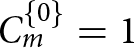$C_m^{\{0\}}=1$ $\mu F.\text{cm}^{-2}$.

We set the value of $\sigma^2$ in the definition of log-likelihood to be $\sigma^2 =1/800$ and perform 5300 iterations in MCMC.

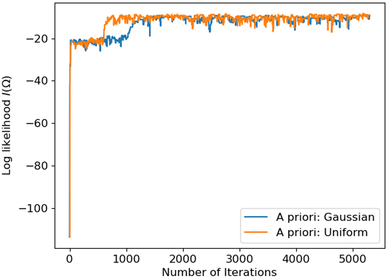
The results shown in Figure 11 demonstrate the stability of the MCMC method under different prior distributions: Gaussian and Uniform. The figure indicates that the performance of the method remains consistent regardless of whether a Gaussian or Uniform prior is used. However, a key advantage of the Gaussian prior is its unbounded support, allowing values to be sampled from $-\infty$ to $\infty$, whereas the Uniform prior samples values within a fixed bounded interval. This characteristic of the Gaussian distribution provides a greater capacity to escape from local optima, thereby improving the robustness of the inference process. In the following analysis, we focus on the results obtained using the Gaussian prior distribution.

Figure 11.

Log likelihood in the MCMC method for unfiltered data.

Based on the results shown in Figure 11, we omit the first 2000 burn-in iterations, to obtain the a posterior distributions of $g_{Na}$, $g_K$, $g_L$, $C_m$ as shown in Figure 12. The estimated values are the values with the highest probability of the posterior distributions which correspond to $g_{Na}=121.49$ $\mu.\text{mho}.\text{cm}^{-2}$, $g_K=12.55$ $\mu.\text{mho}.\text{cm}^{-2}$, $g_L=0.0018$ $\mu.\text{mho}.\text{cm}^{-2}$, $C_m=3.86$ $\mu F.\text{cm}^{-2}$. The corresponding traces are shown in Figure 13.

Figure 12.

Parameters’ posterior distributions of the unfiltered data.

Figure 13.

Parameters’ traces for the unfiltered data.

Using the estimated parameters above, we calculate the firing rates of the HH model and compare to the measured data as illustrated in Figure 14. We can observe that the response of estimated HH model correctly describes the nonlinearity of the PA. This study thus provides a fundamental theory for the J2C scheme proposed in [Reference Wang, Özçelikkale and Benlarbi-Delai15] that the PA network can intelligently process the data set as an NN.

Figure 14.

Comparison of the original non-filtered data and the simulated frequency by estimated data. Left: randomly chosen 1000 points; right: Total 10000 data points.

We perform the same estimation for the filtered data. The total number of the filtered data is 1000000 and we randomly select 5000 data points for the parameter estimation. The initial values of the parameters are also $g_{Na}^{\{0\}}=120$ $\mu.\text{mho}.\text{cm}^{-2}$, $g_K^{\{0\}}=36$ $\mu.\text{mho}.\text{cm}^{-2}$, $g_L^{\{0\}}=0.3$ $\mu.\text{mho}.\text{cm}^{-2}$, $C_m^{\{0\}}=1$ $\mu F.\text{cm}^{-2}$. The value of $\sigma^2$ in the definition of log-likelihood is $\sigma^2 =1/4000$. And we perform 10700 iterations in MCMC.

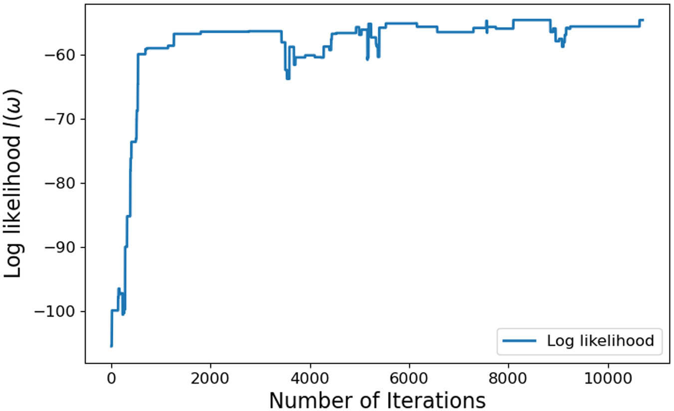
Figure 15 shows the trace plot of the log-likelihood. We omit the first 3000 burn-in iterations and obtain the posterior distributions of the parameters, as shown in the Figure 16. The estimated values as $g_{Na}=45.54$ $\mu.\text{mho}.\text{cm}^{-2}$, $g_K=17.26$ $\mu.\text{mho}.\text{cm}^{-2}$, $g_L=0.176$ $\mu.\text{mho}.\text{cm}^{-2}$, $C_m=1.49$ $\mu F.\text{cm}^{-2}$. Using these estimated parameters, we compute the firing rates of the HH model and compare to the measured data as illustrated in Figure 17. We can see that the HH model can describe nonlinear behavior well but not memory effects, as can be seen from the thickness of the blue curve [Reference Liu, Boumaiza, Sesay and Ghannouchi28]. Thus, further studies are needed on the impact of memory effects on NN computation in the framework of J2C scheme under the scenario that the bandwidth of the processed signal is wider than the allocated frequency range. It is also interesting to explore how the memory effects of the PA can be utilized in AI computing thanks to recursive NN techniques, including state space model (SSM) [Reference Albert, Goel and Ré29] and long short-term memory (LSTM) [Reference Hochreiter30].

Figure 15.

Log likelihood in the MCMC method for filtered data.

Figure 16.

Parameters’ posterior distributions of the filtered data.

Figure 17.

Comparison of the original filtered data and the simulated frequency by estimated data. Left: randomly chosen 5000 points; right: Total 1000000 data points.

In Table 2, we make a comparison among parameter estimation methods with the state-of-the-art, namely LS, Simulated Annealing (SA), and BE. LS is simple and efficient for models that are differentiable and have accessible gradients. However, as a point estimation method, it does not account for uncertainty quantification in parameter estimates, and is prone to getting stuck in local minima. SA, in contrast, does not require gradients and can handle non-differentiable models. Its probabilistic exploration of the parameter space makes it robust against local minima. However, as another point estimation method, it lacks uncertainty quantification. Additionally, it requires careful tuning of annealing parameters, which can increase the computational cost.

Table 2.

Comparison of different parameter estimation methods

The problem we consider introduces the following challenges: the HH model is nonlinear, and there is no analytical formula of the firing rate as a function of the parameters; as a result, it has a complex cost landscape and does not provide gradient. BE overcomes these issues by using a probabilistic framework and provides uncertainty quantification via posterior distributions.

We applied both SA and BE for parameter estimation. We observed that BE yielded more accurate results, reflected in a smaller error compared to SA. This improvement is likely because BE uses a probabilistic approach that takes data uncertainty and noise into account through the posterior distribution. By using the most likely value from the posterior distribution as our estimated parameter, BE fits the data effectively while also accounting for the variability caused by noise. In contrast, SA searches for a single point estimate without explicitly modeling data uncertainty, which may limit its ability to generalize when observational noise is significant.

By the BE, the errors $\epsilon$ defined in (9) for both non-filtered and filtered datasets are presented in Table 3 in linear unit and in decibel (dB), which is computed as

\begin{equation*}\epsilon_\text{dB} = 10\times \log_{10}(\epsilon).\end{equation*}

Table 3.

Modeling accuracy of HH for different datasets measured on PA

The NMSE value with BE for pHEMT PA modeling is around -15 dB, which corresponds to an error ratio of approximately 3%, and for Doherty PA is around -11.5dB corresponding to 7%. This low error indicates that the input-output characteristics of the pHEMT PA closely replicate those of a biological neuron, whereas the Doherty PA may exhibit slightly different types of nonlinear behavior that deviate from biologically plausible nonlinearities. The network of PA can reliably emulate the NN with high fidelity, supporting its use as a functional analog of a biological neuron in neuromorphic computing applications. We have also tested modeling performance with LIF, which gives an NMSE value at -16.9 dB corresponding to an error of approximately 2%. We remark that in the region of high values of external current, there are a few dots of simulated data that do not perfectly fit the measured data. Some inherent relations among the values of the parameters may need further investigation.