
1. Introduction
Phase change materials (PCMs) can store and release a large amount of thermal energy during melting or solidification, practically without changing the temperature. At present, latent heat storage using PCMs is very promising and is used actively in industrial, medical and domestic applications (Biwole, Eclache & Kuznik Reference Biwole, Eclache and Kuznik2013; Ma et al. Reference Ma, Zhang, Ji, Han, Ding and Xie2021; Hayat et al. Reference Hayat, Chen, Bevilacqua, Li and Yang2022; Liu et al. Reference Liu, Hammami, Trovalet, Bigot, Habas and Malet-Damour2022b). The rapid development of space technology imposes high demands on the thermal management system used in space exploration. PCMs have been used in manned space applications since the days of Apollo (Morea Reference Morea1988), and their utilization is growing constantly. The weight of a vehicle can be reduced greatly by temporarily storing energy on board and releasing it when there is excess. The usage of PCMs in spacesuits and astronaut gloves for the work outside the International Space Station has been commercialized for ground-based applications (NASA 2012). Future programmes of the European Space Agency aim to use the capabilities of PCMs to control temperature and provide heat storage capacity; for example, the use of PCMs is foreseen in the Moon Village programme (Williams et al. Reference Williams, Paige, Greenhagen and Sefton-Nash2017).
Selection of a PCM for a space application among a range of possible materials has indicated that organic PCMs made of paraffinic compounds are the most attractive (Collette et al. Reference Collette, Rochus, Peyrou-Lauga, Pin, Nutal, Larnicol and Crahay2011). After analysing nine paraffins, Collette et al. (Reference Collette, Rochus, Peyrou-Lauga, Pin, Nutal, Larnicol and Crahay2011) suggested that n-octadecane is one of the best candidates, due primarily to the highest value of latent heat, low volume change during melting, and stability of its properties. The thermal diffusivity is another important parameter for PCM charge and discharge, as it can limit the amount of energy that would be stored during the orbital period. Even though the thermal conductivity of n-octadecane in a liquid state is not very high, it remains a top candidate. This work is focused on the analysis of heat transfer enhancement in n-octadecane during the melting phase. The Prandtl number of n-octadecane, which defines the ratio of kinematic viscosity to thermal diffusivity, is  $Pr=52.5$.
In terrestrial applications, the presence of convective flows in the liquid phase helps to solve the problem of PCM low thermal conductivity. Extensive research on the subject since the 1980s has shown that convective motions caused by density gradients can enhance the heat transfer rate by about an order of magnitude compared to conductive heat transfer (Sparrow & Broadbent Reference Sparrow and Broadbent1982; Jones et al. Reference Jones, Sun, Krishnan and Garimella2006; Dhaidan & Khodadadi Reference Dhaidan and Khodadadi2015; Madruga & Curbelo Reference Madruga and Curbelo2018; Liu et al. Reference Liu, Zhang, Zhang, Xi, Yuan and Cao2022a). However, this approach is not applicable in microgravity. As an alternative strategy, the use of the thermocapillary effect – in which a non-uniform temperature induces surface tension gradients that drive convective motion – has been proposed as a source of convective heat transport in microgravity PCM devices (Madruga & Mendoza Reference Madruga and Mendoza2017a,Reference Madruga and Mendozab). A possible improvement in heat transfer due to thermocapillary (Marangoni) convection was verified in parabolic flight experiments (Ezquerro et al. Reference Ezquerro, Bello, Salgado Sánchez, Laveron-Simavilla and Lapuerta2019, Reference Ezquerro, Salgado Sánchez, Bello, Rodriguez, Lapuerta and Laveron-Simavilla2020; Salgado Sánchez et al. Reference Salgado Sánchez, Ezquerro, Porter, Fernández and Tinao2020b) and confirmed by numerical simulations (Salgado Sánchez et al. Reference Salgado Sánchez, Ezquerro, Fernández and Rodríguez2020a, Reference Salgado Sánchez, Ezquerro, Fernández and Rodriguez2021; Šeta et al. Reference Šeta, Dubert, Massons, Gavalda, Bou-Ali and Ruiz2021a,b, Reference Šeta, Dubert, Prats, Gavalda, Massons, Bou-Ali, Ruiz and Shevtsova2022).
The common shapes of the PCM containers under investigation are rectangular cavities and squares (Madruga & Mendoza Reference Madruga and Mendoza2020; Martínez et al. Reference Martínez, Salgado Sánchez, Porter and Ezquerro2021), spherical capsules, tubes or cylinders (Šeta et al. Reference Šeta, Dubert, Massons, Sánchez, Porter, Gavaldà, Bou-Ali and Ruiz2021a,b; Varas et al. Reference Varas, Salgado Sánchez, Porter, Ezquerro and Lapuerta2021), and annular cavities (Dhaidan & Khodadadi Reference Dhaidan and Khodadadi2015). The use of thermocapillary force implies the presence of a liquid–gas interface; in this respect, the configuration of a liquid bridge is advantageous, since the shape of the interface can be kept straight easily in microgravity. Literature on liquid bridges reports evidence that when the thermal stresses exceed the critical value, the flow undergoes a transition to oscillatory instability in the form of hydrothermal waves. Depending on the distance from the critical point, liquid properties, geometry and ambient conditions, the liquid bridge system admits the coexistence of waves with different wavenumbers (Shevtsova, Melnikov & Legros Reference Shevtsova, Melnikov and Legros2003; Yasnou et al. Reference Yasnou, Gaponenko, Mialdun and Shevtsova2018), or the emergence of two different modes with different symmetries (i.e.  $m = 0$ and
 $m = 1$) (Shevtsova, Melnikov & Nepomnyashchy Reference Shevtsova, Melnikov and Nepomnyashchy2009; Gaponenko et al. Reference Gaponenko, Yasnou, Mialdun, Nepomnyashchy and Shevtsova2021a). The numerical and experimental investigation of high Prandtl liquid bridges is well advanced in the laboratory (Liang et al. Reference Liang, Jin, Yang, Shi and Zhang2020; Fukuda et al. Reference Fukuda, Ogasawara, Fujimoto, Eguchi, Motegi and Ueno2021; Gaponenko et al. Reference Gaponenko, Yano, Nishino, Matsumoto and Shevtsova2022; Stojanović, Romano & Kuhlmann Reference Stojanović, Romano and Kuhlmann2022) and in microgravity conditions (Kawamura et al. Reference Kawamura, Nishino, Matsumoto and Ueno2012; Schwabe Reference Schwabe2014; Yano et al. Reference Yano, Nishino, Ueno, Matsumoto and Kamotani2017, Reference Yano, Nishino, Matsumoto, Ueno, Komiya, Kamotani and Imaishi2018; Kang et al. Reference Kang, Wu, Duan, Hu, Wang, Zhang and Hu2019).
The change in geometry is inherent to the melting process and solid/liquid front evolution, and it occurs in all PCM geometries, such as rectangular cavities, trapezoidal containers, etc. Recently, a first attempt was made to match the flow dynamics in rectangular liquid containers with those observed during melting (Salgado Sánchez et al. Reference Salgado Sánchez, Porter, Ezquerro, Tinao and Laverón-Simavilla2022). Since the thermal gradients along the PCM/air interface are large, with an increase in the PCM liquid phase, the system is prone to oscillatory instability. Accordingly, in systems with melting/solidification, one can observe the evolution of the nonlinear dynamics inherent in liquid bridges (Lappa & Savino Reference Lappa and Savino2002; Lappa Reference Lappa2018; Varas et al. Reference Varas, Salgado Sánchez, Porter, Ezquerro and Lapuerta2021).
The flow regimes in the melting bridge analysed by Šeta et al. (Reference Šeta, Dubert, Massons, Gavalda, Bou-Ali and Ruiz2021a,b) revealed the appearance of hydrothermal waves (HTWs) in a liquid volume of more than 80 %, except for a narrow region of thermal stresses  $27\ {\rm K} < \Delta T<35 {\rm K}$, where this occurs in a liquid fraction of about 65 %. The standing waves (SWs) are the first to appear (Šeta et al. Reference Šeta, Dubert, Prats, Gavalda, Massons, Bou-Ali, Ruiz and Shevtsova2022), but they decay quickly in favour of travelling waves (TWs). The dynamics of the melting bridge was explored under assumption of an adiabatic free surface. However, extensive experimental and theoretical studies of liquid bridges (Watanabe et al. Reference Watanabe, Melnikov, Matsugase, Shevtsova and Ueno2014; Melnikov et al. Reference Melnikov, Shevtsova, Yano and Nishino2015; Yano et al. Reference Yano, Maruyama, Matsunaga and Nishino2016; Romanò & Kuhlmann Reference Romanò and Kuhlmann2019; Yano & Nishino Reference Yano and Nishino2020) have shown that the heat transfer rate across the interface and the temperature of the surrounding gas can significantly change the supercritical thermocapillary flow and pattern selection. In this work, we extend the previous results on the melting bridge with a more detailed nonlinear analysis of wave properties, and consider the effect of heat transfer across the PCM/air interface on pattern selection and heat transfer rate.
The paper is organized as follows. The mathematical model with appropriate boundary conditions is formulated in § 2. Section 3 is devoted to general characteristics of a stationary flow, such as heat transfer rate and melting dynamics. Section 4 includes a detailed analysis of an oscillatory flow and HTWs. Concluding remarks are presented in § 5.
2. Mathematical model
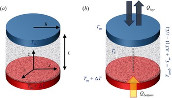
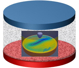
PCM is confined in a cylindrical volume of length  $L$ and radius
 $R$, as shown in the sketch in figure 1. The aspect ratio, defined as length to radius, is kept constant,
 $\varGamma =L/R=1$,
 $L=10$ mm and
 $R=10$ mm. The thermophysical properties of n-octadecane, a high Prandtl liquid, can be found in table 1. The heat influx from the hot disk initiates the melting process. Once PCM on a free surface is melted, the temperature gradient along the liquid part of the interface is established. The surface tension
 $\sigma$ of a liquid is temperature-dependent and defined as
 \begin{equation} \sigma = \sigma_{ref} -\sigma_T(T-T_{ref}) ,\end{equation}
where  $\sigma _T=({\rm d}\sigma /{\rm d}T)_{T_{ref}}$ is the surface tension gradient coefficient, and
 $T_{ref}=T_m+\Delta T/2$. The temperature gradient creates a surface tension gradient at a growing liquid/air interface that induces a thermocapillary flow in the melted liquid and surrounding air (although the latter is not considered). This convection provides a mechanism for heat transport in microgravity, which modifies the melting dynamics and heat transfer via the free surface. The phase change is investigated at several applied thermal stresses
 $\Delta T$, and the associated dimensionless parameter is the Marangoni number
 \begin{equation} Ma= \sigma_T L\,\Delta T/\mu_l \alpha_l. \end{equation}
Since the working liquid and geometry are selected (see table 1),
 \begin{equation} Ma=3149.6\,\Delta T. \end{equation}
Sketches of (a) the geometry and (b) the thermal environment of a melting bridge. A cylindrical volume filled with n-octadecane (the PCM) is held at constant cold ( $T_M$) and hot (
 $T_m+ \Delta T$) temperatures on opposite disks (where
 $T_m=299.65$ K is the melting temperature). The initial temperature of PCM inside the bridge is solidus temperature
 $T_s=298.25$ K. The linear temperature profile is set in ambient air.

Thermophysical properties of the n-octadecane according to Madruga & Mendoza (Reference Madruga and Mendoza2017a). Here,  $\sigma _T=({\rm d}\sigma /{\rm d}T)_{T_{ref}}$ and
 $\alpha _l=\lambda _l/\rho _l c_{p,l}$. The subscripts
 $m$,
 $l$ and
 $s$ stand for the melt, liquid and solid, respectively.

2.1. Governing equations
The flow dynamics of the system is described by the momentum and continuity equations for incompressible Newtonian fluids, with sink term in the momentum equation, which differentiates the velocity between the solid and liquid phases. The system is considered in the microgravity environment, thus gravity is absent ( $g = 0$):
 $$\begin{gather} \partial_t{\boldsymbol u} + ({\boldsymbol u} \boldsymbol{\cdot} \boldsymbol{\nabla}) {\boldsymbol u} =- \frac{1}{\rho_0}\,\boldsymbol{\nabla} p + {\nu}\,\nabla^2 {\boldsymbol u}+ \frac{1}{\rho_0}\, \frac{C(1-\gamma)^2}{\gamma^3+b}\,{\boldsymbol u} , \end{gather}$$
 $$\begin{gather}\boldsymbol{\nabla} \boldsymbol{\cdot} {\boldsymbol u} = 0, \end{gather}$$
where  ${\boldsymbol u}$ represents the velocity vector
 ${\boldsymbol u}=(u, v, w)$,
 $p$ is the buoyant pressure (the difference between total and hydrodynamic pressures),
 $\rho _0$ is the density at a reference temperature
 $T_{ref}$, and
 $\nu =\mu _l/\rho _0$ is the kinematic viscosity. The last term on the right-hand side of the momentum equation (2.4) represents the Carman–Kozeny model for a moving solid–liquid interface as a porous mushy layer where solid and liquid phases may coexist (Egolf & Manz Reference Egolf and Manz1994). Thus a single momentum equation is solved for both liquid and solid phases (the solid one is fixed in place).
The conservation of thermal energy takes into account the heat transfer and the phase change (latent heat  $\Delta H$):
 \begin{equation} \partial_t (c_p T) + {\boldsymbol u} \boldsymbol{\cdot} \boldsymbol{\nabla} (c_pT) = \frac{1}{\rho}\,\nabla^2 (\lambda\,T) - \Delta H\,\frac{\partial \gamma}{\partial t}, \end{equation}
where  $c_p$ and
 $\lambda$ are the weighted specific heat and thermal conductivity of liquid, defined as
 $$\begin{gather} \lambda=(1-\gamma)\lambda_{s}+\gamma \lambda_{l} , \end{gather}$$
 $$\begin{gather}c_p=(1-\gamma)c_{p,s}+\gamma c_{p,l} , \end{gather}$$
with the subscripts  $l$ and
 $s$ denoting ‘liquid’ and ‘solid’, respectively. The density across phases is constant, which means that the volume remains constant too.
The enthalpy-porosity formula combines the momentum, continuity and energy equations to describe the evolution of the phase change process. The important point of the model is the definition of the liquid fraction field,  $\gamma$, since it provides the coupling between the momentum and energy equations. This field depends on temperature and is constrained between 0 (a pure solid) and 1 (a pure liquid). In the regions where the solid and liquid are mixed together, the so-called mushy regions, the liquid fraction is not well-defined and should be approximated. The common approach for modelling the liquid fraction in mushy regions is to use a linear interpolation between the solidus temperature
 $T_s$ and the liquidus temperature
 $T_m$. Thus the liquid volume fraction in the bridge,
 $\gamma$, is defined as
 \begin{equation} \gamma = \left\{ \begin{array}{@{}ll} 0, & T \le T_s, \\ \dfrac{T-T_s}{T_m-T_s}, & T_s< T< T_m, \\ 1, & T\ge T_m. \end{array} \right. \end{equation}
The Darcy constant  $C$ in (2.4) is set to
 $C=1.6\times 10^6$ kg s m
 $^{-3}$; see Madruga & Mendoza (Reference Madruga and Mendoza2017a). This constant depends on the material's mushy region morphology, but generally has a high value in the range between
 $10^3$ and
 $10^9$. As can be seen from (2.4), when
 $\gamma \to 0$ (solid phase), the Darcy term tends to a very high value ensuring no-flow conditions in that region, while when
 $\gamma = 1$, this term disappears. The small constant
 $b=10^{-3}$ is added to this term to prevent division by zero when
 $\gamma =0$; its choice is arbitrary.
2.2. Boundary and initial conditions
The dynamic deformation of the PCM air/liquid interface is not taken into account, which is justified by the smallness of the capillary number  $Ca=\gamma \,\Delta T/\sigma _T$, and is about 0.1 at the maximum temperature gradient used in this study.
1. The PCM/gas interface
 $r=R$: the balance of viscous and thermocapillary forces and kinematic condition for a non-deformable interface are imposed:
(2.10)where\begin{equation} \mu\,\frac{\partial {\boldsymbol u}} {\partial n} = \sigma_T\,\frac{ \partial T}{\partial \tau}, \quad {\boldsymbol u}_n=0, \\ \end{equation}$\partial /\partial n$ and $\partial /\partial \tau$ are the derivatives in the normal and tangential directions.
The heat transfer through the interface is described as
(2.11)The Biot number is defined as\begin{equation} \frac{\partial T}{\partial n}=Bi\,(T-T_{amb}), \quad T_{amb}=T_{m}+\Delta T(1-z/L).\end{equation}$Bi=h R/\lambda _{l}$, where $h$ is the heat transfer coefficient. The idea of presenting the results in terms of the dimensionless Biot number is substantiated as follows. Presumably, the coefficient $h$ under microgravity conditions is small, since there is no natural convection, and the forced convection in air, caused by the moving interface due to the Marangoni effect, is weak (Shevtsova, Gaponenko & Nepomnyashchy Reference Shevtsova, Gaponenko and Nepomnyashchy2013). The common estimation for $h$ in the case of forced convection starts from 10 W ${\rm m}^{-2}\ {\rm K}^{-1}$ (Kosky et al. Reference Kosky, Balmer, Keat and Wise2013). Since the exact values of $h$ are unknown, we propose to consider the heat transfer in terms of the Biot number, which characterizes the conduction resistance inside a body with respect to heat convection at the surface. In this work, the Biot values have been chosen ranging from 0.5 to 3 in order for both effects to be important. In addition, this provides a range of $h$ values from 6.5 to 39 W ${\rm m}^{-2}\ {\rm K}^{-1}$ (see table 1), which is in good agreement with the proposed estimation by Kosky et al. (Reference Kosky, Balmer, Keat and Wise2013).
The ambient temperature is set as a linear profile along the free surface. The temperature profile in air near the interface was measured experimentally in a somewhat similar configuration (Shevtsova, Mialdun & Mojahed Reference Shevtsova, Mialdun and Mojahed2005). The results showed a temperature drop on the solid supports, while the rest of the interface had a linear profile.
2. The top and bottom of the domain
$z=0$, $z=L$: no-slip impermeable boundary conditions for velocity are imposed. The system is heated from below, and the temperature on the upper support is equal to the melting point:
(2.12a–c)\begin{equation} {\boldsymbol u}=0, \quad T(z=0)=T_m+\Delta T, \quad T(z=L)=T_m=299.65\ {\rm K}. \end{equation}3. Zero pressure gradient is considered on all the walls:
(2.13)\begin{equation} { \partial P}/{\partial n}=0.\\ \end{equation}4. Initial conditions: the melting bridge is in solid state and kept at constant solidus temperature
$T_s=298.25$ K, which is 1.4 K lower than that of the upper support ($T_m$). If the temperatures were equal, then the narrow zone close to the cold wall would remain solid. In addition, the region between $T_m$ and $T_s$, called the mushy region, helps to ensure numerical stability as there are no abrupt changes in thermophysical/transport properties.


2.3. Numerical method
The model is implemented in the open source software OpenFOAM. The cylindrical geometry of the melting bridge is discretized with a Cartesian mesh. In order to do this, the cylindrical domain has to be split into multiple domains, avoiding singularity in the central point of the cylinder. First, the core central part is chosen to be an octagon, as it has relatively smooth edges and makes the mesh cylindrical-like. The choice of the way the mesh is split plays an important role in the evolution of the flow dynamics, where, for example, the square central core part can favour an even wavenumber of modes (Aguilar Reference Aguilar2011; Šeta et al. Reference Šeta, Dubert, Prats, Gavalda, Massons, Bou-Ali, Ruiz and Shevtsova2022). Time step  $\Delta t$ has been assigned dynamically to accomplish the condition
 $Co<0.5$, where
 $Co=u_{max}\,\Delta t/\Delta x$ is the Courant number, the indicator of numerical stability, and
 $\Delta x$ is the length of the numerical cell.
2.4. Convergence of numerical solutions
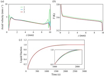
The convergence of the numerical simulations is examined for three different mesh choices in table 2. The meshes are compared and characterized by the number of cells, simulation cost (in time for 100 s), melting time to achieve 50 % and 99 % liquid fractions, and deviations with respect to the finest mesh used. Since one of the goals of this work is to analyse the effect of thermocapillary convection during the PCM melting, it is natural to use the melting time as an indicative value for checking numerical convergence.
Results of the mesh convergence test for numerical simulations at  $\Delta T=25$ K. The selected mesh is mesh 2; deviations in the melting time for 50 % and 99 % liquid fractions are calculated with respect to mesh 3.

A comparison of the interface velocity calculated at different meshes in figure 2(a) illustrates that our mesh has a slight twisting on the cold side, which does not affect characteristics of interest in this study such as the melting time and the oscillation frequency. To avoid this twisting, the regularization of boundary conditions is often used in the literature, after Wanschura et al. (Reference Wanschura, Shevtsova, Kuhlmann and Rath1995). A close analysis leads to the conclusion that the regularization cuts out this twisting artificially, and in the end, in both cases a similar modification of the flow is introduced. The finest mesh does not have such a twisting, but the calculation time is enormously large. Note that we also made simulations between our mesh and the finest one, and the twisting was still present.
Mesh convergence test. (a) Velocity at the interface. (b) Temperatures at the interface. The temperature scale is reduced to emphasize the difference. (c) Evolution of the liquid fraction with time. The inset presents a magnified view to illustrate the difference between the meshes as the system approaches complete melting. The selected mesh is in blue.

The temperature distribution along the interface on the selected mesh is smooth and practically coincides with the finest mesh. The difference in the evolution of the melting time can be noticed only under magnification; see figure 2(c). The level of the numerical error for the melting time with this choice is below 2.5 %, which is coherent with typical experimental uncertainties. The validation with the existing experiments in the literature has been done in our previous works (Šeta et al. Reference Šeta, Dubert, Massons, Gavalda, Bou-Ali and Ruiz2021a,b, Reference Šeta, Dubert, Prats, Gavalda, Massons, Bou-Ali, Ruiz and Shevtsova2022). In all the cases, mesh 2 (blue curves) is found to offer a good compromise between a reduced computational cost and numerical accuracy.
2.5. Digital signal processing
For frequency analysis, the fast Fourier transform has been calculated using a Hanning window of 2048 points, which gave a frequency resolution of the order of 0.5 mHz. To obtain the power spectral density evolution, records of 50 s delayed by 1 s between them were used systematically.
3. Results: heat transfer rate and melting dynamics
3.1. Balance of heat transfer
To determine the time evolution of the heat transfer rate through the upper (cold) and lower (hot) supports of the melting bridge, the local heat flux  $q=-\lambda \,\partial T/\partial z$ is integrated over the disk surface
 $A$:
 \begin{equation} Q =-\lambda \int_A (\partial T/\partial z)_{z=0, L}\,{\rm d}A, \end{equation}
where  $\lambda$ is the thermal conductivity of phase in contact with the support (
 $\lambda =\lambda _s+(\lambda _l-\lambda _s)f$, with
 $\lambda _s$ and
 $\lambda _l$ being the thermal conductivity of the solid and liquid phases respectively, and
 $f$ the liquid fraction). According to the direction of the
 $z$-axis, a positive value of
 $Q_{bottom}$ indicates a heat flux entering the melting bridge through the hot disk. Correspondingly, a positive value of
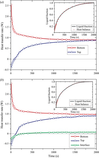
 $Q_{top}$ shows a heat flux leaving through the upper disk. Figure 3(a) presents the time evolution of
 $Q_{top}$ and
 $Q_{bottom}$ for adiabatic conditions (
 $Bi=0$) and
 $\Delta T=25$ K. As can be seen, heat always enters the melting bridge through the lower support and decreases rapidly as the melting process proceeds. At the initial stage, heat also enters through the upper disk, since the temperature of the bulk was first set to
 $\sim$1 K below the temperature of the cold disk, but then it reverses, and the bridge loses heat. The unbalanced heat (
 $Q_{melt}=Q_{bottom}-Q_{top}$) is absorbed by the PCM to melt. When the PCM is completely melted, the rate of heat transfer through both supports collapses to a value 0.882 W; see figure 3(a). Comparison of this value with that expected from a pure conductive state,
 $Q_{cond}=\lambda _l A\,\Delta T/L=0.102$ W, shows that in the liquid bridge, the heat transfer by the convection is 8.6 times more efficient than that provided by the heat conduction.
Heat transfer rate through the bottom, the top and the interface of the liquid bridge at  $\Delta T=25$ K when (a)
 $Bi=0$ and (b)
 $Bi=3$. The insets illustrate the temporal evolution of the liquid fractions
 $f$ and
 $f_{b}$ obtained by two different approaches: direct numerical simulation and (3.2). Here,
 $Ma=3149.6\,\Delta T$.

The analysis of the heat transfer behaviour for the other values of  $\Delta T$ reveals a similar tendency, but a steady state is reached earlier as
 $\Delta T$ grows, since the PCM is melted faster. The role of convection becomes more important as
 $\Delta T$ increases. Note that the heat transfer rate through solid substrates in the presence of convection and in the case of pure conduction increases with
 $\Delta T$, but to a different extent. This leads to a growth of the convective/conductive transfer ratio: i.e.
 $Q_{bottom}(t\to \infty )/Q_{cond}= 7$ (
 $\Delta T=18$ K), 8.6 (
 $\Delta T=25$ K) and 9.1 (
 $\Delta T=40$ K). Comparing these values, one can conclude that this ratio, which characterizes the improvement in heat transport due to convection, reaches a plateau with an increase in
 $\Delta T$.
To check the robustness of the calculations, the liquid fraction  $f_{b}$ is determined from the heat balance as
 \begin{equation} f_{b}(\tau)=\frac{\displaystyle \int_0^{\tau} (Q_{bottom}-Q_{top})\,{\rm d}t}{\displaystyle \int_0^{\infty} (Q_{bottom}-Q_{top})\,{\rm d}t}. \end{equation}
The comparison of the time evolution for  $f$ obtained in the course of simulations as a mean value at a given time, and
 $f_{b}$, is presented in the inset of figure 3(a). The figure illustrates good agreement between the evolutions of the liquid fractions determined by different approaches.
Under non-adiabatic conditions, the cylindrical PCM/air interface also takes part in the energy balance; in particular, after melting of a solid phase, heat goes across the liquid/gas interface. The heat flux through the unit of the free surface area ( $q$) and the total heat transfer through the interface (
 $Q_{int}$) are written as
 \begin{equation} q=-\lambda_l\left.\partial T/\partial r\right|_{r=R}=h (T_{int}-T_{amb}), \quad Q_{int}=-\lambda_l \int_{A_l} q\,{\rm d}A, \end{equation}
where  $h$ is the heat transfer coefficient at the liquid–gas interface,
 $(T_{int}-T_{amb})$ is the difference between the interfacial and ambient temperatures, and
 $A_l$ is the lateral surface area of the liquid bridge.
The heat flux through the interface is considered positive when the melting bridge loses heat. The temporal evolution of  $Q_{int}$ is shown in figure 3(b) for
 $Bi=3$ (
 $h=39\ {\rm W}\ {\rm m}^{-2}\ {\rm K}^{-1}$) and
 $\Delta T=25$ K, in addition to
 $Q_{top}$ and
 $Q_{bottom}$. The rates of heat transfer through both solid substrates behave similarly to those observed in the adiabatic case, but in the non-adiabatic case they are not equal in the steady state. Comparison of figures 3(a) and 3(b) shows that
 $Q_{bottom}$ (the red curve) is almost the same, while the heat flux through the top (the blue curve) is initially higher in the non-adiabatic case. This can be understood in a way that initially heat enters the system also through the interface, because over most of the liquid bridge height the ambient temperature is higher than inside. Over time, heat gain through the PCM/gas interface decreases, mainly due to the thermal Marangoni effect, which heats and melts the solid/gas interface in tens or hundreds of seconds. A careful inspection of figure 3(b) shows that the heat flux through the interface,
 $Q_{int}$, changes sign from negative to positive at
 $t\sim 250$ s. This occurs when the free surface becomes hotter than the ambient temperature. When the entire PCM is melted, the heat transfer rates are
 $Q_{bottom}=0.972$ W,
 $Q_{top}=0.904$ W and
 $Q_{int}=0.083$ W. Note that
 $Q_{int}$ is only 9 % of the conductive term. In the non-adiabatic case, the heat transfer rate through the disks is slightly higher than that corresponding to the adiabatic case (
 $Q_{bottom}=Q_{top}=0.882$ W).
The inset of figure 3(b) presents the comparison between the evolution of the liquid fraction obtained directly from the numerical code and that computed from the heat balance. As in the adiabatic case, the minor differences existing between the results are a consequence of the cumulative numerical errors.
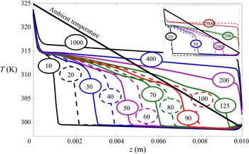
Figure 4 shows temperature profiles along the free surface of the melting bridge at selected times (indicated on each profile). In the earlier stages of the melting, a significant part of the surface is colder than the melting temperature, which leads to heat gain from the ambient gas. Later, at  $t\sim 125$ s, the thermal front with
 $T=T_{melt}$ reaches the cold disk (
 $z=0.01$ m), which means complete melting of the solid phase near the free surface. This situation provides a favourable scenario for convective heat transfer through the free surface without being limited with still unmelted solid part. The mean surface temperature becomes higher than the mean ambient temperature, which leads to a sign change of
 $Q_{int}$. Reaching the steady state, the central part of the interface has a nearly uniform temperature of about 316 K, with large gradients near both ends, which correspond to heat gain through the hot support of the bridge and heat loss through the cold part. To better characterize the effect of the interface temperature on the heat flux balance, the inset of figure 4 shows a comparison between the axial temperature profiles for the non-adiabatic and adiabatic cases. As long as there is a heat gain from the air (
 $t<250$ s), the surface temperature in the non-adiabatic case is higher than the temperature corresponding to
 $Bi=0$. The situation reverses at later times, when the bridge starts to lose heat to the air. Note that in the adiabatic case, the thermal front moves slower than in the non-adiabatic case. As
 $\Delta T$ increases, the general behaviour of the fluxes is preserved, but as in the adiabatic case, the relevant parameters are slightly readjusted. For example, at
 $\Delta T=40$ K and
 $Bi=3$,
 $Q_{bottom}=1.715$ W and
 $Q_{top}=1.545$ W; the latter is similar to that obtained for the adiabatic case at
 $\Delta T=40$ K. Because of the faster dynamics of the melting, the heat flux through the interface becomes positive earlier than in the
 $\Delta T=25$ K case,
 $t=150$ s versus 250 s. In addition,
 $Q_{int}(t\to \infty )=0.108$ W, which is significantly higher than the value obtained for
 $\Delta T=25$ K.
Axial surface temperature profiles at selected times for  $\Delta T=25$ K,
 $Bi=3$. The thick straight line represents the temperature in the ambient gas. The inset shows the comparison between the profiles for adiabatic (dashed line) and non-adiabatic (solid line) profiles.

3.2. The thermal performance of PCM
One of the most important parameters in the thermal performance of PCM is the amount of heat that can be removed from the hot source at a given time interval. Several approaches can be developed to quantify the efficiency of the heat removal process. For a two-dimensional parallelepiped configuration, Martínez et al. (Reference Martínez, Salgado Sánchez, Porter and Ezquerro2021) used the so-called enhancement factor, which is the ratio of the melting times in the adiabatic and non-adiabatic cases. They found that this enhancement factor increases with the  $Bi$ number.
In order to quantify the performance of the heat extraction in liquid bridge geometry, we propose to determine the mean heat transfer rate through the hot (lower) support during a given time  $t_1$:
 \begin{equation} Q_{mean}=\frac{1}{t_1} \int_0 ^{t_1} Q_{bottom}\,{\rm d}\tau. \end{equation}
We analyse two values of the time interval  $t_1$. First, we set
 $t_1 = 400$ s in order to study the system in the initial phase of melting, when a significant part of the PCM is still solid. Next, we set
 $t_1=2000$ s to evaluate the long-term performance, i.e. to determine the amount of heat removed from the system when the PCM is completely melted.
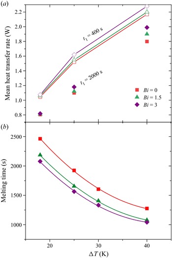
Here, we consider a dynamics of melting with a linear temperature profile in the ambient gas, which changes the heat transfer and the melting process. Figure 5(a) exhibits that the mean heat transfer rate  $Q_{mean}$ increases considerably with
 $\Delta T$, which is expected. The effect of the Biot number on the heat transfer rate through the hot support is much weaker and depends on time. The role of the Biot number at
 $t=2000$ s is more pronounced than at
 $t=400$ s. It is interesting to note that the mean heat transport decreases at longer times, reflecting the reduction of the efficiency as the PCM becomes more melted. This is clearly seen in figure 5(a), where the solid symbols are much lower than the open ones. These latter results suggest the advantage of removing the melting bridge from a source of heat before the complete melting is achieved. This strategy can improve the performance of heat removal by up to 20 %. In our opinion, this may be associated with the structure and inclination of powerful HTWs at the final stage of melting. The connection between the shape of liquid/solid interface interface and heat transfer at the solidification stage was discussed by Lappa & Savino (Reference Lappa and Savino2002).
(a) Mean heat transfer rate  $Q_{mean}$ through the lower (hot) support at different stages of the melting process (
 $t_1= 400$ s and 2000 s) as a function of
 $\Delta T$ and the Biot number. The line-connected open symbols correspond to
 $t_1=400$ s, and the solid symbols without a guide line correspond to
 $t_1=2000$ s. (b) Decrease of the complete melting time with
 $\Delta T$ at different
 $Bi$. The relation between the Marangoni number and
 $\Delta T$ is
 $Ma=3149.6\,\Delta T$.

The importance of heat transport across the PCM/air interface is nearly negligible at  $\Delta T=18$ K for all
 $Bi$, and grows with
 $\Delta T$. The slight enhancement of
 $Q_{mean}$ with an increase in
 $Bi$ can be associated with the activation of the Marangoni convection due to the heat transfer through the interface, which helps the conduction mechanism.
3.3. Dynamics and topology of the melting front
The overall dynamics of the melting time with  $Bi$ and
 $\Delta T$ is shown in figure 5(b). It is seen that the melting process is slowest in the adiabatic case. Comparison of the curves for
 $Bi=0$ and
 $Bi\neq 0$ indicates that the appearance of heat transfer through the interface essentially decreases the melting time, but depends a little on the value of the Biot number, at least in the explored range
 $1< Bi<3$. The effect of the Biot number is most noticeable at the smallest
 $\Delta T$, and is practically the same for different Biot numbers when
 $\Delta T$ reaches 40 K. Our results support previously reported data by Martínez et al. (Reference Martínez, Salgado Sánchez, Porter and Ezquerro2021) for a cavity that the Biot number accelerates the melting.
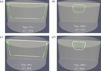
The topology of the melting front can be traced in figure 6. In the earliest times, heat transfer is dominated by conduction, and the melting front propagates parallel to the hot supports, and much faster at the bottom. Gradually, the thermocapillary force induces convection in a small region near the interface. At the interface, the Marangoni flow is directed from the hot part to the cold part, and accelerates melting in the hot corner region. This is well illustrated by figures 6(a) and 6(c), where the melting front penetrates deeper towards solid at the bottom at  $t\sim 100$ s (175 s). The thin melting zone propagates rapidly up along the interface as it is enhanced by the convective flow caused by the surface tension gradient due to the existing temperature difference. In a relatively short time, the melting front forms two directions: from the interface to the inner region, driven by the Marangoni convection, and from the bottom to the top, driven by thermal conduction. On the short time scale (figures 6a,c), the effect of the Biot number is insignificant (compare the white and green curves). Slight advancement of the melting process (green curves for
 $Bi=3$) visible at the upper part occurs due to the enhancement of convection by the ambient gas; see the temperature distribution in figure 4. There is no Biot effect on the melting front in the lower part, since the thermal field is controlled by thermal conduction from the hot support. In later times (figures 6b,d), the topology of the melting front changes. Although the same two directions of the melting front are clearly visible, their relation to interfacial heat transfer is different. The melting front, moving from the bottom (or top) is practically not affected by the Biot number, as the temperature field remains to be dominated by the hot (cold) support. Accordingly, the green and white curves have the same location at the top and bottom. Thermocapillary convection creates a quicker heat transport than conduction, resulting in faster progress of the solid/liquid interface perpendicular to the free surface. The melting front, governed by Marangoni convection, is affected strongly by heat transfer across the interface.
Topology of the melting front at different times for  $Bi=0$ (white) and
 $Bi=3$ (green) at
 $\Delta T=25$ K and
 $\Delta T= 40$ K.

Figures 6(b,d) demonstrate that melting occurs faster at  $Bi\neq 0$. The reason for the faster melting dynamics lies in the modification of the temperature profile and, more importantly, temperature gradients on the interface. When the heat loss becomes essential (e.g.
 $Bi=3$), the gradients near the solid supports are getting sharper, while they are more flat in the central part (Melnikov & Shevtsova Reference Melnikov and Shevtsova2014; Melnikov et al. Reference Melnikov, Shevtsova, Yano and Nishino2015). It results in the enhancement of convection and faster melting.
4. Results: oscillatory flow
4.1. Onset time of an oscillatory flow
The difference in the evolution time of the liquid fraction at various Biot numbers appears at rather late times when Marangoni convection develops, i.e.  $t>500$ s (
 $\Delta T=25$ K) and
 $t>400$ s (
 $\Delta T=40$ K); see figure 7. At the earlier times, a quick advance of the liquid fraction occurs due to enhanced conductive transport within the solid phase of PCM since the thermal conductivity of the solid phase is higher than that of the melt. With the predominance of the PCM liquid phase, melting slows down and the role of convection activated by the Biot number increases. The most distinct role of various Biot numbers is observed at the moments when more than 80–90 % of PCM is melted. Approximately at these moments, the convective flow undergoes transition from stationary to oscillatory. The onset of oscillations is indicated by the crosses on the curves in figure 7.
Evolution of the liquid fraction with time at different Biot numbers. The crosses indicate the beginning of the oscillatory regime: (a)  $\Delta T=25$ K and (b)
 $\Delta T =40$ K.

The study of the oscillatory flow regimes is based on the nonlinear dynamics of the temperature field. This is because temperature signals are more accessible in the course of experiments in a liquid bridge. Furthermore, the dynamic characteristics of the flow field are similar to the thermal ones. To follow the development of the oscillatory regime, a point located on the lateral surface close to the hot support at  $z=0.1 L$ is selected. The time signals in this point were recorded continuously with the following spectral analysis as described in § 2.5. On the basis of the spectral analysis, the onset time of the oscillatory regime was determined.
A summary of the data on the emergence of oscillations is presented in figure 8. In the adiabatic case, for relatively low  $\Delta T$, such as
 $\Delta T=18$ and 25 K, the stationary flow persists longer until oscillations occur. The opposite situation is observed at higher
 $\Delta T$, i.e.
 $\Delta T\ge 30$ K, when the Biot number delays the appearance of the oscillatory flow. It should be noted that in this
 $\Delta T$ range, the Biot number comes into play only for sufficiently strong heat transfer through the interface,
 $Bi>1$.
Onset time of an oscillatory flow as a function of Biot number at different  $\Delta T$.

4.2. Properties of HTWs
Above the critical  $\Delta T_{cr},$ a time-periodic three-dimensional flow
 ${\tilde F}$, at leading order, can be represented as
 ${\tilde F}\approx F_0+{F},$ where
 $F_0$ is the stationary flow, and
 ${F}$ is the oscillatory part. A three-dimensional oscillatory flow emerges in the form of two waves propagating in opposite directions, and the solution of the linearized problem can be written as
 \begin{equation} \left.\begin{array}{c@{}} {F}=a_+F_+ + a_-F_-,\\ \mbox{where}\quad F_{{\pm}}={\hat F}_{{\pm}}(r,z)\exp({\rm i}m\phi {\pm} {\rm i}\omega t)+{\rm c.c.} \end{array}\right\} \end{equation}
Here,  $a_+$ and
 $a_-$ are the arbitrary coefficients,
 $m$ is the azimuthal wavenumber, and
 $\omega =2 {\rm \pi}/f$ is the angular frequency. Usually, one observes either an SW,
 $a_- = a_+$, or a TW, while one of the amplitudes
 $a_{\pm }$ vanishes. For the sake of simplicity of the discussion, we neglect the multiple frequencies. To examine the properties of an HTW, we follow a recently developed methodology (Gaponenko et al. Reference Gaponenko, Yasnou, Mialdun, Nepomnyashchy and Shevtsova2021b).
In the supercritical region, the time periodic solution contains the entire spectrum of wavenumbers,  ${-\infty }< m<{-\infty }$, but only a few modes have a significant amplitude. According to the Fourier spectra shown later, in figure 12, the solution is time-periodic, with the form
 \begin{equation} F=\sum_{m=-\infty}^{\infty}\sum_{n=-\infty}^{\infty}\hat{f}_{m,n}(r,z) \exp({\rm i}m\phi+{\rm i}n\omega t), \end{equation}
where  $\hat {f}_{-m,-n}=\widehat {f^*}_{m,n}$,
 $m$ is the wavenumber, and
 $n$ is the number of the combinational Fourier harmonic for that component with wavenumber
 $m$. Note that the wavenumber in a cylindrical liquid bridge is an integer.
In the following, we are interested in the azimuthal wavenumber and properties such as whether the wave is travelling or standing. To examine the properties of an HTW with a given azimuthal number  $m$, the perturbation quantity
 $\tilde f$ is decomposed into real and imaginary parts at a fixed horizontal position. Then (4.2) is written in the suitable form
 \begin{equation} F= \sum_{{ m=}-\infty}^{\infty}{\tilde f_m}(r,z,t)\exp({\rm i}m{\phi}). \end{equation}
For further analysis, we consider only the non-axisymmetric part of the solution,  $\tilde f,$ which can be determined from the computed quantity
 $\tilde F(r,\phi, z)$ by subtracting the average field as
 \begin{equation} {\tilde f}(r,\phi, z,t)=\tilde{F}(r,\phi, z,t) - \frac1{2{\rm \pi}} \int_0^{2{\rm \pi}} \tilde F(r,\phi, z) \,{\rm d}\phi. \end{equation}
Then the perturbation quantity  ${\tilde f}$ is decomposed into real and imaginary parts at fixed horizontal position
 $z=\bar {z}$ for each
 $m$:
 \begin{align} F_m(t)&= \frac1A \int_0^{R}\int_0^{2{\rm \pi}}{\tilde f}(r,{\phi, \bar{z}},t)\, {\rm e}^{-{\rm i}m{\phi}}\,r\, {\rm d}r\,{\rm d}\phi\nonumber\\ & =\int{\tilde f}(r,{\phi, \bar{z}},t)\cos(m{\phi})\,r \,{\rm d}r \, {\rm d}{\phi} - {\rm i}\int {\tilde f}(r,{\phi, \bar{z}},t) \sin(m{\phi})\,r \,{\rm d}r \, {\rm d}{\phi} \nonumber\\ &= {\rm Re}[F_m(t)] - {\rm i}\,{\rm Im}[F_m(t)], \end{align}
where  ${\tilde f}$ can be any of
 ${\boldsymbol V}, P, T;$ we select
 $\tilde f$ to be associated with the temperature of the liquid. For the graphical representation of
 ${\rm Re}[F_m(t)]$ and
 ${\rm Im}[F_m(t)]$, they are divided by the cross-sectional surface area (
 $A={\rm \pi} R^2$). The observation of the prescribed temperature displacement with time (e.g. the position of a point on the trajectory in the phase plane) is performed from a two-dimensional steady state. The steady state in the plot is the origin of coordinates (point
 $(0,0)$) where
 ${\rm Re}[F_m(t)] = {\rm Im}[F_m(t)]=0$. In the case of a TW, the trajectory during one oscillation period forms a circle centred at point
 $(0,0)$. In the case of an SW, the trajectory appears as a straight line crossing the centre.
4.3. Hydrothermal waves at $\Delta T=25$ K

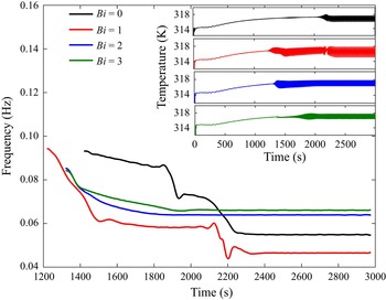
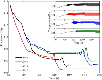
The approach presented above has been applied to the analysis of an HTW in a liquid bridge by Gaponenko et al. (Reference Gaponenko, Yasnou, Mialdun, Nepomnyashchy and Shevtsova2021a,Reference Gaponenko, Yasnou, Mialdun, Nepomnyashchy and Shevtsovab). Recent studies of melting bridges (Šeta et al. Reference Šeta, Dubert, Massons, Gavalda, Bou-Ali and Ruiz2021a,b, Reference Šeta, Dubert, Prats, Gavalda, Massons, Bou-Ali, Ruiz and Shevtsova2022) have shown that their nonlinear flow dynamics is more complex than in liquid bridges without melting. The evolution of the melting bridge dominant frequency over time at different Biot numbers is shown in figure 9 at  $\Delta T=25$ K. The frequency analysis starts from the moment of emergence of oscillations and continues until the completion of the entire melting process where the system reaches steady-state oscillations. First inspection of figure 9 indicates that for all the Biot numbers, the main frequency decreases continuously in time. This decrease is explained by the permanent increase in the liquid volume during the melting process. At an earlier stage of the process, the frequency decreases rapidly as the melting occurs rapidly; see figure 7. Over time, the growth rate of the liquid fraction slows down and, accordingly, the frequency changes more slowly. Sharp drops in frequency evolution are associated with changes in nonlinear dynamics of the system, for example, with the changes in the wavenumber of an HTW.
Evolution of the main frequency during the melting process and beyond at  $\Delta T=25$ K. Different colours are attributed to various Biot numbers. The insets illustrate the progress of the temperature oscillations.

The inset in figure 9 displays the time evolution of the temperature oscillations. Clearly, the growth of the amplitude at onset depends on the Biot number and  $\Delta T$. In most of the cases presented, the amplitude increases continuously with time, although sometimes it decreases and even may vanish for a short period of time. The sharp changes in the amplitude are consistent with jumps of the frequency in the main plot. The onset of oscillatory instability is determined from the information in the insets of the temperature oscillations.
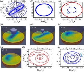
The emergence and evolution of HTWs are closely related to the transient behaviour of the frequency. We start the discussion about HTWs from  $Bi=0$. Figure 9 reveals the birth of a frequency
 $f\sim 0.09$ Hz at
 $t=1450$ s, which slowly decreases until
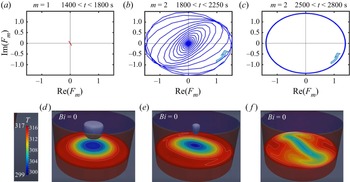
 $t=1800$ s. The corresponding tiny temperature oscillations are barely noticeable in the inset. The methodology presented in § 4.2 clearly shows that these low-amplitude oscillations correspond to an HTW with azimuthal wavenumber
 $m=1$; see figure 10(a). In the considered time interval, the trajectory of
 $m=1$ is a straight line passing through the origin of the phase plane, which is the signature of the SW. The black curve in figure 9 illustrates that later, there is a long two-step frequency drop, which lasts from
 $t=1800$ s until
 $\sim 2250$ s. During this time, the SW is attenuated and a spiral wave is originated, the development of which leads to the formation of a TW with
 $m=2$, as can be seen in figure 10(b). Also during this stage, the final melting of the solid PCM takes place. At an even later time (see figure 10c), a uniform TW with
 $m=2$ is established, which is characterized by the trajectory in the form of a circle centred at the origin of coordinates. Over time, the TW keeps a constant frequency and an oscillation amplitude, as follows from figure 9. The constancy of the temperature pattern and wave properties can be attributed to a completely melted PCM. Figures 10(d–f) present the temperature fields at the same times as the trajectories. The isolines in cross-sections help us to understand the structure of HTWs, while the dark blue three-dimensional drawings show the solid part of PCM.
Trajectories of the dynamic system at different time intervals when  $Bi=0$ and
 $\Delta T=25$ K, illustrating: (a) SW
 $m=1$; (b) transition between dynamic states; and (c) developed TW with
 $m=2$. (d–f) Corresponding temperature patterns. The dark blue three-dimensional shapes illustrate the non-melted PCM.

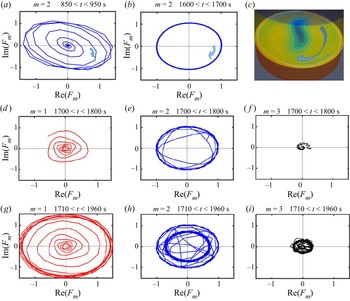
Nonlinear dynamics of the system is more complicated in the non-adiabatic case. Let us consider the behaviour of the system when  $Bi=1$. In order to explore the system dynamics, one should simultaneously follow the spectral characteristics shown by the red curve in figure 9 and the trajectories in figure 11. From the onset of an oscillatory state, its frequency decreases continuously at a sufficiently large rate, while the amplitude of the temperature oscillations rises. At this time, the trajectory of the HTW winds up and forms a circle that has the features of a future TW with
 $m=2$, as seen in figure 11(a). Later, i.e. at
 $t\approx 1500$ s, the decrease rate of the frequency diminishes. The phase plane exhibits pronounced features of a TW with
 $m=2$. However, since the frequency is not constant, the trajectories continue winding on a circle with a little divergence in figure 11(b).
(a–c) Trajectories of the dynamic system at different time intervals when  $Bi=1$ and
 $\Delta T=25$ K: (a) HTW with growing amplitude; (b) developed TW with
 $m=2$; and (c) the final state with coexistence of two TWs with different
 $m$, where both waves travel in the clockwise direction. (d–f) Snapshots of temperature field at times corresponding to (a–c), where the dark blue three-dimensional shapes illustrate the non-melted PCM. (g–i) Details of the transition from uniform TW with
 $m=2$ to HTW with mixed modes:
 $m=1$ and
 $m=2$ with a smaller amplitude.

The next big changes in the frequency behaviour are observed at the time interval  $2100 < t < 2300\ {\rm s}$. The dynamic behaviour becomes intriguing, and for clarity, the transient regime is detailed by three graphs in the bottom row, in figures 11(g–i). At these moments, the TW with
 $m=2$ loses its power, the amplitude of its oscillations decreases, and this gives a chance for the birth of a more energetic TW with
 $m=1$. Finally, the frequency stabilizes and the trajectories of two TWs settle in the phase plane, the more energetic one with
 $m=1$, and the weaker one with
 $m=2$. Both waves travel in the same clockwise direction. Snapshots of the temperature field in figures 11(d–f) are given for the same time instants as the trajectories in figures 11(a–c). They make clear that the emergence of
 $m=1$ and the weakening of
 $m=2$ occur after complete melting of PCM. The constant radii of the trajectories in figure 11(c) indicate that the amplitude and frequency of oscillations do not change in time, and the patterns will be stable in a rotating frame of reference, since one revolution corresponds to one oscillation period, while the observer is in the centre of the plane,
 $({\rm Re}(F_m),{\rm Im}(F_m))=(0,0)$.
The Fourier spectra in figure 12, characterizing the oscillatory behaviour of the system, clearly distinguish one fundamental frequency with additional peaks corresponding to the frequencies  $2f_1, 3f_1$, therefore the solutions are periodic in time.
Fourier spectra in the time interval 2500–2900 s when  $\Delta T=25$ K: (a)
 $Bi=0$,
 $f_1=0.046$ Hz,
 $f_2=2f_1$,
 $f_3=3f_1$; (b)
 $Bi=3$,
 $f_1=0.066$ Hz,
 $f_2=2f_1$,
 $f_3=3f_1$.

Supplementary movie 1 (available at https://doi.org/10.1017/jfm.2023.463) accompanies figure 11, showing the temporal evolution of the flow pattern and trajectories of the system in the phase plane at  $\Delta T=25$ K and
 $Bi=1$.
4.4. Hydrothermal waves at $\Delta =40$ K

For  $\Delta T=40$ K, we explore in detail the case with
 $Bi=3$. For this, one should analyse simultaneously the green curves in figure 13 and the whole of figure 14. The melting time is rather fast,
 $t\sim 1000$ s, and the oscillatory regime sets in shortly before the complete melting, i.e. at
 $t \approx 900$ s as seen in figure 7(b). The green curve inset in figure 13 exhibits that after a short initial time interval, the temperature oscillations retain a constant amplitude for a long time, until
 $t\sim 1800$ s. During the initial stage, when the amplitude and frequency of oscillations are settling, the trajectory of the emerging TWs is an unwinding spiral; see figure 14. With time, this spiral turns into a uniform TW with
 $m=2$, rotating clockwise. Later, at
 $t \approx 1800$ s, the amplitude of oscillations decreases sharply to almost zero, and then rapidly increases; see the green curve inset in figure 13. Usually, this is associated with a transition between oscillatory states.
Evolution of the main frequency during the melting process and beyond, at  $\Delta T=40$ K and various Biot numbers. The insets illustrate the evolution of of the temperature oscillations.

Trajectories of the dynamic system at different time intervals when  $Bi=3$ and
 $\Delta T=40$ K. (a–c) Here,
 $t\le 1600$ s: formation of TW, developed TW with
 $m=2$ and flow pattern at
 $z=3$ mm illustrating TW rotating clockwise. (d–f) Here, the different stages of HTWs are shown at
 $t = 1800\ {\rm s}$: (d) birth of
 $m = 1$; (e) reverse of the rotation direction of the primary TW with
 $m = 2$ to counterclockwise; (f) birth of TW with
 $m = 3$ rotating clockwise. (g–i) Here,
 $t=2000$ s: coexistence of three TWs with
 $m=1$,
 $m=2$ and
 $m=3$.

Indeed, this moment corresponds to a total change in the nonlinear dynamics of the system. The fundamental frequency makes a couple of kinks and drops sharply. The long-lived TW with  $m=2$ starts to lose power and changes the direction of rotation; see figure 14(e). This stressful system behaviour triggers two additional HTWs,
 $m=1$ and
 $m=3$ as shown in figures 14(d,f). In general, their trajectories in the phase plane resemble a logarithmic spiral, when the distance between successive turns of the spiral increases. However, the nature of their spiral growth is very different. Spiral-like wave with
 $m=1$ unwinds counterclockwise, which is consistent with the
 $m=2$ new direction of rotation. The less energetic
 $m=3$ performs small coils that make up a spiral-like wave. Furthermore,
 $m=3$ rotates in the clockwise direction, which is opposite to
 $m=1$ and
 $m=2$.
Later, at  $t\sim 2000$ s, the system behaviour stabilizes. The final dynamic pattern of the system consists of three TWs, which are shown in figures 14(g–i): the most energetic TW with
 $m=1$ and the weakened TW with
 $m=2$ rotate counterclockwise; the less energetic TW with
 $m=3$ rotates clockwise.
4.5. Summary of nonlinear dynamics of a melting bridge
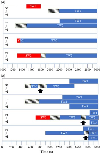
Figure 15 summarizes, in terms of Biot number and time, the evolution of nonlinear dynamics of the melting bridge at low and high thermal stresses, for  $\Delta T=25$ K and
 $\Delta T=40$ K. Standing waves exist only at the onset of instability and at selected Biot numbers. Later, over time, they break up in favour of TWs. If, for a given Biot number, an SW does not emerge at the onset of instability, then a spiral wave arises, which winds up and leads to the formation of a TW. At earlier times, for all the studied
 $\Delta T$, a TW appears with a dominant azimuthal wavenumber
 $m=2$. At low thermal stresses,
 $\Delta T=25$ K, only at
 $Bi=1$ is the primary TW accompanied by the secondary mode
 $m = 1$, and both rotate in a clockwise direction. For other Biot numbers, TW with
 $m=2$ is the only one that exists during the observation time. At high thermal stresses,
 $\Delta T=40$ K, the primary TW with
 $m=2$ is accompanied later in time by one or two other TWs with
 $m=1$ and
 $m=3$. The overall nonlinear dynamics becomes more complicated at high thermal stresses; over time, the primary TW can change direction (these moments are shown by the arrows in figure 15), and the TWs emerging later can have opposite directions of rotation.
Summary of nonlinear dynamics of melting bridge. Emergence of HTWs in time for  $Bi=0$, 1, 2 and 3 for (a)
 $\Delta T=25$ K, and (b)
 $\Delta T=40$ K. TW stands for travelling wave, SW for standing wave, and the last digit indicates the oscillatory mode
 $m$. Shaded areas indicate phases of formation of TW2 waves, and arrows indicate time moments when wave changes the direction of rotation. Supplementary movie 2 (
 $Bi=1$,
 $\Delta T=40$) and supplementary movie 3 (
 $Bi=2$,
 $\Delta T=40$) are available by clicking on the shadow regions for the selected
 $Bi$.

Supplementary movie 2 ( $Bi=1$,
 $\Delta T=40$) and supplementary movie 3 (
 $Bi=2$,
 $\Delta T=40$) are available by clicking on the shadow regions in figure 15 for the selected
 $Bi$, which show the coexistence and transitions of three modes with different
 $m$ and the transition from SWs to TWs.
5. Conclusions
This paper presents a detailed three-dimensional numerical investigation of melting dynamics of the phase change material (PCM) n-octadecane ( $Pr = 52.5$) subjected to thermocapillary effects. The dynamics of phase-change transition in microgravity is modelled using an enthalpy-porosity based formulation of the Navier–Stokes equations coupled with the energy equation. The PCM is enclosed in a cylindrical container, and the temperature difference
 $\Delta T$ between the lower (hot) and upper (cold) solid supports is applied. The lateral surface is in contact with air, the temperature of which changes linearly. As soon as a part of the lateral surface melts, the thermocapillary effect causes convection in an initially small area. The melting process is enhanced locally and accelerates the advancement of the solid/liquid front along the lateral boundary. When the liquid fraction occupies
 $\sim$80–90 % of the volume (depending on
 $\Delta T$), the flow undergoes transition from stationary to oscillatory. The properties of emerging HTWs in an oscillatory regime are analysed using recently suggested methodology (Gaponenko et al. Reference Gaponenko, Yasnou, Mialdun, Nepomnyashchy and Shevtsova2021a,Reference Gaponenko, Yasnou, Mialdun, Nepomnyashchy and Shevtsovab). The effects of heat transfer through the interface on the nonlinear dynamics are studied at different Biot numbers.
From the results obtained, it can be concluded that thermocapillary convection allows enhancing the heat transfer rate of n-octadecane by a factor of 7–9 compared with pure thermal conduction when  $\Delta T$ changes from 18 K to 40 K. This dependence is not linear, and as
 $\Delta T$ increases further, the improvement reaches a plateau.
Curiously, heat loss through the interface increases the average heat transfer ( $Q_{mean}$) through the hot support, albeit only slightly. The enhancement in
 $Q_{mean}$ with an increase in
 $Bi$ can be associated with the activation of Marangoni convection due to a change in the interface temperature. Another interesting finding is that
 $Q_{mean}$ decreases at later times (for example, at 400 s versus 2000 s), reflecting a decline in efficiency as the liquid fraction increases considerably. This suggests disconnecting the PCM system from the hot source before the PCM is completely melted.
Melting time is another important factor for PCM performance. The presence of heat transfer through the interface essentially decreases the melting time, but depends little on the value of the Biot number. The effect of the Biot value is most noticeable at the smallest  $\Delta T$, and is almost negligible when
 $\Delta T$ reaches 40 K. An analysis of the topology of the melting front reveals two somewhat independent mechanisms of its propagation: (a) driven by thermal conduction, when the front is parallel to the hot/cold substrate, and (b) driven by convection, when the front is perpendicular to the interface. The latter is affected by the Biot number.
We have paid special attention to the nonlinear evolution of HTW by means of Fourier analysis and building trajectories of various modes in the phase plane to identify SWs and TWs and their azimuthal wavenumber. As a general statement, it is worth noting that TW with  $m=2$ is the dominant HTW in the nonlinear dynamics of a melting bridge.
A detailed analyses of HTW properties at  $\Delta T=25$ K indicates that, with the exception of
 $Bi=1$, an SW emerges at the onset of the oscillatory regime. However, this wave lives for only a short time and is replaced by a TW with the azimuthal wavenumber
 $m=2$. The latter wave persists throughout the observation time. Again, as an exception at
 $Bi=1$, the
 $m=1$ mode appears at a much later time and coexists with
 $m=2$.
The nature of the coupling between HTW and Biot number is more complicated at high thermal stresses. At  $\Delta T=40$ K, an SW appears only at
 $Bi=2$. In all the other cases, the formation of HTWs begins with a spiral-like wave that unwinds clockwise and leads to the formation of a TW with
 $m=2$. Later, other TWs with
 $m=1$ and
 $m=3$ emerge, which affect the primary TW with
 $m=2$. As the result of such an interplay, a TW with
 $m=2$ can weaken (a decrease in the amplitude in the phase plane) and/or change direction of rotation.
Supplementary movies
Supplementary movies are available at https://doi.org/10.1017/jfm.2023.463.
Funding
The present work has been supported by grants 2021PFRURV- 74 (Rovira i Virgili University), MMASINT (KK-2023/00041) and IT1505-22 (Research Group Program) of the Basque Government, and PID2020-115086GB-C33 and PID2020-115086GB-C32 financed by (MICINN/FEDER) of the Spanish Government.
Declaration of interests
The authors report no conflict of interest.