1. INTRODUCTION
A fractal layout is defined as a factory within a factory, where several fractal cells are formed by different types of machines (Ozcelik & Islier, Reference Ozcelik and Islier2003). The main goal is to execute the different types of operations in the fractal cell that had been previously chosen, eliminating any long travels on the shop floor. Basically, in this type of layout, the traveling distance is composed of intercellular trip and intracellular trip distances. The first case occurs when a requested machine is allocated on the other fractal cell, and then workpieces are left from one fractal cell to reach the other. The second case occurs when the requested machine is allocated in the same fractal cell but it is located in a different position. Thus, the way machines are allocated on the shop floor and the order of how fractal cells are selected and positioned have a significant importance in traveling distance minimization.
In this research paper, we propose to allocate similar fractal cells as far as possible to obtain a reduced intercellular traveling distance, in a feasible computational time. A fractal cell similarity-based methodology is proposed to design fractal layouts by allocating cells on the shop floor. The concept of similarity between fractal cells was firstly cited by Montreuil et al. (Reference Montreuil, Venkatadri and Rardin1999). According to them, although all cells aim to process all products, each cellular layout has been specialized for different ratios of the product mix. Two cells are considered independent if no intercellular travel occurs between them. Two cells are considered similar if they are expected to process more or less the same products in the same quantities. Nevertheless, researchers have not proposed a procedure to solve this issue in fractal layout. We also explore the possibility of virtual cells formation in a fractal cell aiming to minimize the intracellular traveling distance. Thus, some issues must be analyzed: the allocation of fractal cells and machines, the division of operations of each workpiece in k parts in order to simulate intercellular traveling distance, the definition of virtual cells in each fractal cell, and the definition of criteria for choosing fractal cells for manufacturing workpieces (we adopted the selection based on the closest distance and on the highest similarity).
This paper is organized as follows: in Section 2, we report some of important procedures proposed in the literature for the fractal layout design, showing the differences among them, commenting on the results obtained and the conclusions. In Section 3, the adopted mathematical model is presented aiming to minimize intertravel and intratravel distances. Next, we present our procedures to separate machines among fractal cells (in a balanced or unbalanced way), to identify the similarity of fractal cells and to allocate it on the shop floor, for which we develop a Tabu search based heuristics. In addition, a Tabu search based heuristics is used to identify the best sets of machines in the selected fractal cell for a specific set of workpieces. In Section 4, a case study is presented to test our proposed procedures, where workpieces and layouts are generated and submitted to simulation. Following, we compare the performances among functional, distributed, and fractal layouts. Finally, the conclusions are described in Section 5.
2. LITERATURE REVIEW
This section aims to present some techniques for designing a fractal layout, discussing how each one works. The first methodology for the designing of fractal layout may be seen in the work of Venkatadri et al. (1997). Their methods consisted in three phases. The first phase aimed to estimate the number of fractal cells. This was obtained by dividing the total number of machines by the types of machines. Based on their approach, basically, fractals cells were randomly selected. After this, the second phase of the methodology consisted in choosing and allocating machines to form each selected fractal cell. Although these authors did not explain exactly how machines were selected and allocated on the shop floor for each fractal cell, we assume this procedure was randomly executed, that is, machines were randomly selected and allocated from top–bottom and from left–right of the shop floor. Finally, the third step consisted in flow assignment, where workpiece sequence was analyzed and traveling distance was calculated. In order to improve the performance, these authors proposed two pairwise exchange-based heuristics to improve the initial layout. First, two machines' positions were changed and traveling distance calculated. If the recent traveling distance calculated was lower, the previous traveling distance calculated was then updated by this recent one. Second, these authors also considered the manner of how fractal cells were allocated among them, because it affects intercellular traveling distance. It occurs when requested machines belong to other fractal cells. The calculation of intercellular traveling distance can be obtained based on the centroid of each fractal cell. These authors presented seven cases studies, comparing the performances of fractal cells to function, cellular, and holographic layouts, which these were considered two performance parameters (number of machines and total traveling distance). The makespan calculation was omitted. In each case study, for each layout type, they adopted a different number of machines for comparison. For instance, for Case 1, they adopted 29 machines for functional layout, 46 for cellular layout, 29 for distributed layout, and 32 machines for fractal layout. They concluded that their proposed method for the design of fractal layouts is computationally feasible in terms of computational time and that their iterative heuristics methods for flow assignments works well in order to improve the initial generated fractal layout.
Saad and Lassila (Reference Saad and Lassila2004) also proposed a methodology to design fractal layouts to reduce intercellular traveling distance. Their proposed methodology aimed to analyze the similarity between workpiece operation and cell capability. The main idea was, because most operations of a certain workpiece would be manufactured in the chosen fractal cell, the result of intercellular traveling distance naturally would be reduced. Hence, the cell with the highest capability was then chosen for manufacturing workpieces. One of the research studies that did not consider this issue was Venkatadri et al. (Reference Venkatadri, Rardin and Montreuil1997). In their research, the selected fractal cell could not pursue the requested machine, which has resulted in an increment of intercellular traveling distance. Saad and Lassila (Reference Saad and Lassila2004) proposed a Tabu search based heuristics to reallocate machines in each fractal cell by changing theirs positions in order to minimize intracellular traveling distance. In addition, fractal cells positions were changed and evaluated. The fractal cell positions that yielded the lowest total traveling distance remained. They concluded that the total traveling distance (intertraveling distance plus intratraveling distance) could be minimized by applying their methodology and also increasing the total number of machines.
Montreuil et al. (Reference Montreuil, Venkatadri and Rardin1999) proposed a few steps in order to a fractal design. Their approach can be described as including the following:
1. a “capacity planning” step, where basically the number of different types of machines was estimated according to the demand of parts. Thus, using the information about the processing time and the availability work shift of each type of machine, the number of replicas can be estimated;
2. a “cell creation” step, which was used to define the type of machine that should belong to which fractal cell;
3. a “flow assignments” step, which analyzed possible routings of each part to machines;
4. a step “cell” for each fractal cell aimed to change machines' positions to others located in the same fractal cell in order to search the lowest routings; and
5. a global layout aimed to reallocate fractal cells to search for the lowest intercellular traveling distance.
Sitorus et al. (Reference Sitorus, Nawangpalupi, Amelia and Wijaya2006) conducted a research paper in which layouts were generated and compared. In general, it could be said that the designing approach used for layout generation was similar to what Venkatadri et al. (Reference Venkatadri, Rardin and Montreuil1997) had proposed. For the evaluation of functional layout, these authors adopted the methodology proposed by Apple (Reference Apple1993), which consisted of three steps: capacity planning (where the number of each type of machine was estimated by dividing the operation time requested by workpieces of that requested machine per total available time per shift), determination of the flow matrix (where number of travels of workpieces between machines was registered), and department exchange (where departments positions were changed in order to obtain any performance improvement). According to the same authors, the procedure for the cellular layout was similar to the one used in the functional layout, except in the cellular layout formation phase, when a machine's clustering procedure for cell creation must be followed. Some clustering measure used by these authors can be seen in Singh and Rajamani (Reference Singh and Rajamani1996). For the fractal layout, the number of fractal cells was estimated, although these authors did not explain how it was done. Next, the machines were allocated to each fractal cell. The machines were probably randomly chosen. Based on this information, the calculation of total flow was done. The flow was computed as follows: for each workpiece, alternatives flows of workpieces were analyzed and the shortest distance remained. They repeated the procedure for all submitted workpieces. Based on the developed Tabu Search heuristics, fractal cells' positions were simply changed and the total distance recalculated. Finally, for holonic layout, the capacity planning step was used as previously described. Next, in order to allocate machines on the shop floor, an invisible curve based on the similarity coefficient (also called the Hilbert curve) was generated. Machines were then randomly selected, and they were allocated by following the obtained curve. First, to obtain the flow material, operations that require the allocated machine are ordered from highest processing time to the lowest. Second, it consisted in identifying the lowest demanded machine. Hence, highest processing time operation was allocated in the lowest demanded machine. The performance parameters adopted to conduct the comparison were number of machines, the flow score, and the mean flow time. These authors presented seven cases studies, in which layouts composed of a different quantity of machines were evaluated (the lowest quantity of machines was 14 and the highest was 60). They concluded that, in general, the fractal layout and the holonic layout offered better performance in comparison to traditional layouts (functional layouts and cellular layouts), because both always gave the lowest flow scores.
Askin et al. (Reference Askin, Ciarello and Lundgren1999) conducted a research performance comparison between distributed layout and fractal layout. They proposed two algorithms for the generation of distributed layouts. The first algorithm, called holonic random, consisted in generating some curves on the shop floor. These curves were also called space filling curves (SFC). Next, machines were randomly selected and allocated by following the generated curves. The second algorithm, called holonic similarity coefficient, was based on the probability of occurrence between processes. That is, machines responsible for consecutive operations were allocated as close as possible. The allocation of machines also followed SFC. For empirical analysis, they evaluated a total of 30 and 60 machines, and each part demanded from 5 up to 15 operations. They concluded that the performance of distributed layout was between the fractal layouts and the functional layouts. Since then, there have been few research projects about fractal layout.
1. In Venkatadri et al. (Reference Venkatadri, Rardin and Montreuil1997), fractal cells were randomly allocated. For each allocated fractal cell, the procedure of flow assignments was randomly repeated several times for each workpiece to find the best workpiece routing. Using the same idea, the procedure was also used in the algorithm proposed by Montreuil et al. (1999). We can raise some issues: the assignment effectiveness could be improved, especially when handling with large number of fractal cells; the chosen fractal cell might not pursue the requested machine, increasing consequently the intercellular traveling distance; and basically one performance parameter was considered (traveling distance), omitting makespan, for instance.
2. The methodology proposed by Saad and Lassila (Reference Saad and Lassila2004) aimed to analyze the similarity between workpieces operation and cell capabilities. This issue was omitted by Venkatadri et al. (Reference Venkatadri, Rardin and Montreuil1997) and Montreuil et al. (Reference Montreuil, Venkatadri and Rardin1999). Nevertheless, fractal cell positions were also changed and evaluated several times. There are several disadvantages of their procedure. When the number of fractal cells increases, the time spent by the CPU may increase significantly owing to the global searching. In other words, the manner in which fractal cells were allocated did not follow any criteria, which means the given fractal cell could be allocated in undesirable places on the shop floor several times. Unfortunately, these authors did not compute the time taken by the CPU. It shows promise if a procedure could be elaborated to allocate large number of fractal cells in a short period of CPU time. They evaluated the performance of the production system (total traveling distance) by varying the total number of machines. Therefore, we can also affirm they considered one performance parameter.
3. Finally, Sitorus et al. (Reference Sitorus, Nawangpalupi, Amelia and Wijaya2006) developed specifically a Tabu Search heuristics, where fractal cell positions were simply randomly changed and the total distance recalculated. Nevertheless, the methodology did not consider the similarity issue between fractal cells, which means that there are unnecessary intercellular travelings, and the proposed method also realized global searching several times.
As we can see, there are already researchers focusing on the design of fractal layout. The current approach usually executes several times the allocations of fractal cells on the shop floor and the flow assignment to find the best one. Because of combinatorial features, a fractal layout with a large number of fractal cells may present a significant disadvantage for efficient allocations. Thus, this paper aims to propose a criterion, based on similarity among fractal cells, developed and implemented in a Tabu search heuristics to obtain the best fractal layout in a feasible computational time.
3. MATHEMATICAL MODEL
In this research work, we aim to solve all previously cited disadvantages. To conduct this research paper, we formulate the following mathematical model in Eq. (1), where the main goal is to minimize the total traveling distance. Note that the adopted objective function z is composed of intracellular and intercellular traveling distances, respectively.
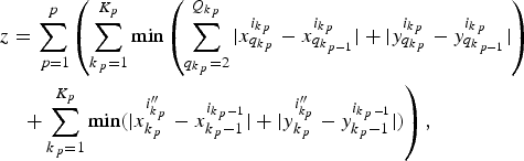 $$\eqalignno{&z = \sum\limits_{\,p = 1}^p \left(\sum\limits_{k_{\,p} = 1}^{K_p} \min \left(\sum\limits_{q_{k_{\,p} }=2 }^{Q_{k_{\,p} } } \vert x_{q_{k_{\,p} } }^{i_{k_{\,p}}} - x_{q_{k_{\,p - 1}}}^{i_{k_{\,p} } } \vert + \vert y_{q_{k_{\,p} }}^{i_{k_{\,p}}} - y_{q_{k_{\,p - 1}}}^{i_{k_{\,p}}} \vert \right)\right.\cr &\quad\left. + \sum\limits_{k_{\,p} = 1}^{K_p } \min \lpar \vert x_{k_{\,p} }^{i^{\prime\prime}_{k_{\,p} } } - x_{k_{\,p} - 1}^{i_{k_{\,p} -1} } \vert + \vert y_{k_{\,p} }^{i^{\prime\prime}_{k_p } } - y_{k_{\,p} - 1}^{i_{k_{\,p}- 1}} \vert \rpar \right)\comma}$$
subject to
 $$x\comma \; y \, \, {\rm integers}\semicolon \;$$
 $$x\comma \; y \gt 0\semicolon \;$$
 $$ \lcub x\comma \; y \rcub \in \lcub 1..X\comma \; 1..Y \rcub \comma \; {\rm respectively}\semicolon \;$$
 $$1 \le i \le n_c\semicolon \;$$
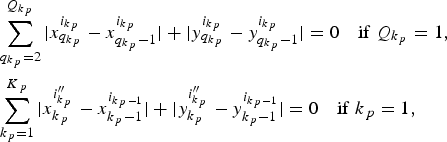 $$\eqalignno{& \sum\limits_{q_{k _{\,p}}=2}^{Q_{k_{\,p }} } {\vert x_{q_{k _{\,p}} }^{i_{k _{\,p}} } - x_{q_{k _{\,p}} - 1}^{i_{k _{\,p}} } \vert +\vert y_{q_{k _{\,p}} }^{i_{k _{\,p}} } - y_{q_{k _{\,p}} - 1}^{i_{k _{\,p}} } \vert =0\quad {\rm if}\ Q_{k_{\,p} }=1}\comma \cr & \sum\limits_{k_{\,p}=1}^{K_{\,p} } {\vert x_{k_{\,p} }^{i_{k_{\,p} }^{{\prime \prime} } } - x_{k_{\,p} - 1}^{i_{k_{\,p} - 1} } \vert +\vert y_{k_{\,p} }^{i_{k_{\,p} }^{{\prime \prime} } } - y_{k_{\,p} - 1}^{i_{k_{\,p} - 1} } \vert =0\quad {\rm if}\ k_{\,p}=1}\comma}$$
 $$i_{k_{p} } \ne i_{k_{p}+1}^{\prime \prime }.$$
The constraint Eq. (2) ensures the use of integer numbers just to simplify the calculation by Hamming distance formula. This approach is the same as used in the quadratic assignment problem (QAP), in which machines are considered as square format of the same sizes and positioned in horizontal and vertical on the shop floor. In addition to this, subsequent machines are separated in one unit of distance (as adopted by Rosenblatt & Golany, Reference Rosenblatt and Golany1992; Benjaafar, Reference Benjaafar1995; Ji et al., Reference Ji, Wu and Liu2006; Pitombeira Neto et al., Reference Pitombeira Neto, Chin and Gonçalves Filho2007; Chin, Reference Chin2013). The calculated distance is given in units of distance. Next, the constraint Eq. (3) is adopted simply to use positive coordinates X and Y. Variables x and y, which represent position of machine allocated on the shop floor, must receive values lower than layout settings X and Y [see the constraint in Eq. (4)]. Variable i represents the chosen fractal cell for manufacturing the q k pth step of the k pth set [see Eq. (5)].
The constraint in Eq. (6) is composed by two parts. The first means that if Q k = 1, no intercellular traveling distance occurs because all operations are carried out in the same chosen fractal cell i. The second means if k demands only one operation in each chosen fractal cell i, no intracellular traveling distance is computed.
After receiving operations (correspondent to subset k p) in the chosen fractal cell i, the workpiece is conducted to the next chosen fractal cell i k p+1′′ to receive the operations for the subset k p + 1. Therefore, the constraint [Eq. (7)] means no backtracking, which ensures that a certain workpiece must leave one fractal cell and reach another for processing next k p, that is, k p + 1.
Next, we present steps adopted in this research paper to design fractal layouts in order to accomplish the objective function [Eq. (1)]:
Step 1. Order types of machines according to number of replicas (from higher to lower).
Step 2. Estimate the number of fractal cells, through n c = T/n, as proposed by Venkatadri et al. (1997). Because it may result in a rational number, we will always truncate n c and then plus one.
Step 3. Quantify the number of machines in the ith fractal cell. We considered two possibilities, in both of which, there is at least one fractal cell pursuing all types of machines. This condition was implemented in order to avoid any deadlocks in the computational model, that is, because the chosen ith fractal cell is based on the similarity, then at least one must pursue all types of machines.
Step 3.1. For an unbalanced number of machines: select a machine (obeying the order established in Step 1) and allocate beginning from the first fractal cell up to n c. If the number of replicas of the chosen machine becomes zero before reaching n c, the next type of machine is chosen and the allocation begins from the first fractal cell; if the number of replicas of the chosen machine is different from zero, the allocation continues up to n c, and continues beginning from the first fractal cell.
Step 3.2. For a balanced number of machines: the first fractal cell receives one replica of each type of machine. No more machines are allocated in this first fractal cell. For each remaining fractal cell (i.e., from the second up to n c), select a random machine. If the replica is different from zero, then the machine is allocated. If the replica is zero, another machine is chosen. Once the n c is reached, if there are machines with replicas different from zero, the allocation begins from the second fractal cell up to n c, and so forth.
Step 4. The main idea is that similar fractal cells should be allocated as far as possible. For doing this, we propose to calculate similarity between fractal cells i in relation to fractal cell i′ through the use of the expression for the calculation of the Jaccard coefficient, such as shown in Eq. (8). The variable i′ represents the fractal cell that is composed by all types of machines (thus S i ′i ′ = 1):
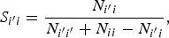 $$S_{i^{\prime}i}=\displaystyle{{N_{i^{\prime}i} } \over {N_{i^{\prime}i^{\prime}}+N_{ii} - N_{i^{\prime}i} }}\comma \;$$
where i ∈{1, … , n c} except i′; N i ′i is the number of machines in common between i′ and i; N i ′i' is the number of machines in common between i′ and i′; and N ii is the number of machines in common between i and i;
Step 5. We intend to calculate the distribution degree, such as proposed by Benjaafar and Sheikhzadeh (Reference Benjaafar and Sheikhzadeh2000), when the formula was applied to obtain the maximally distributed layout. Using the same idea, in order to calculate it, we develop a Tabu Search algorithm. Thus, this step aims to adapt the fractal layout to permit the calculation. It is necessary to define movable intervals G max and G min to evaluate how similar a fractal cell i is in relation to i′. These intervals are obtained by establishing a value for the maximum difference (max_diff) of similarities. The total number of intervals (represented by number_intervals) is estimated by (1/max_diff) + 1, because the highest value of similarity is 1. If the result of the division is an integer number, then for the first interval, G max ←1, and G min = G max – max_diff. The second movable interval is obtained through G max ← G min and G min ← G max – max_diff, and so on up to G min = 0. Otherwise, if the division is a rational number, the estimated number of intervals is the truncate of number_intervals and the movable intervals (except the last one) are also defined through G max ← 1 and G min= G max – max_diff, and so on. Only for the last interval, G max – G min = 1 – (number_intervals * max_diff). Once intervals are defined, compare each value of calculated similarity of fractal cell i to the interval. If the similarity is located in the first interval (i.e., G max ≤ S i ′i < G min), then all machines of that fractal cell i will be renamed to G = 1, and if it is in the second interval, then G = 2, and so forth.
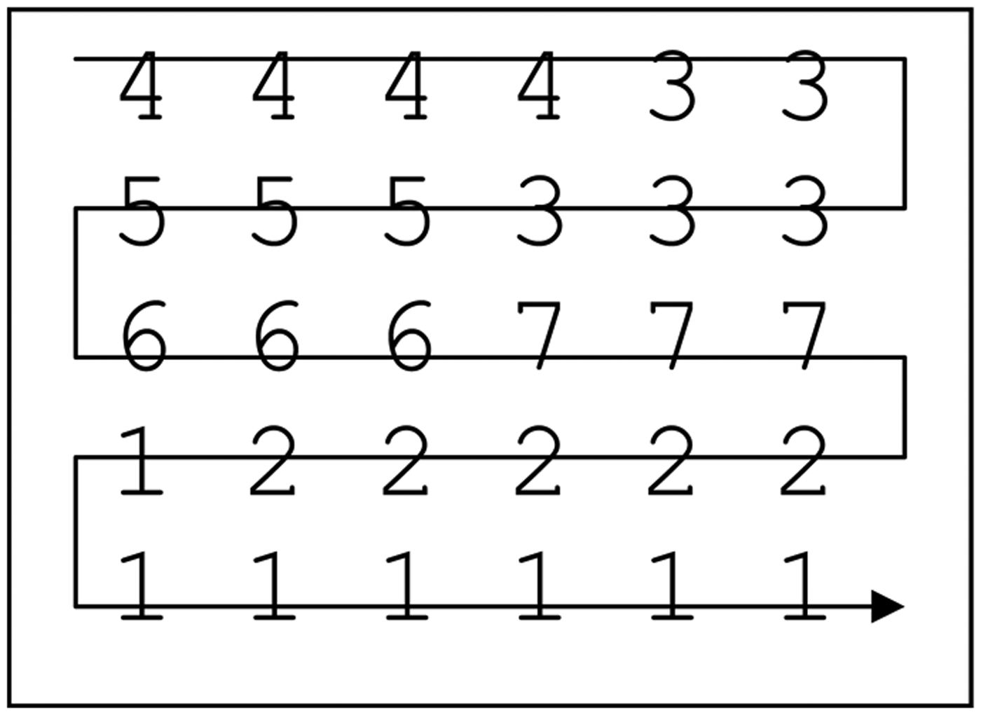
Step 6. Select g ∈ {1..G}, where g has not been previously selected, and allocate all replicas of g on the shop floor, according to X and Y (the format of the fractal layout, where machines are allocated in X horizontal and Y vertical) and obeying the SFC procedure. In this research paper, we adopted the simplest one, where machines are allocated from top to down and from left to right. Repeat Step 6 for all G.
Step 7. In order to attend the objective function minmax (proposed by Francis & White, Reference Francis and White1974; and adapted by Benjaafar & Sheikhzadeh, Reference Benjaafar and Sheikhzadeh2000), also called distribution degree, the computational model is initially designated to search positions for replicas of g.
Step 8. Calculate the distance among different fractal cells from the centroid. It can be done by identifying the position of each replica g and then calculating the mean distance between each g of different fractal cells. Repeat it for other g. Keep the layout that yields the lowest distribution degree aiming at allocating that each g belongs to a different fractal cell as far as possible.
Step 9. Repeat Steps 6, 7, and 8 Tabu_allocation_cells times.
Step 10. Reidentify the machines (i.e., convert each g), such as defined by the Step 3.
Step 11. Separate operations of each workpiece p into K subsets, in which each k is composed by subsequent operations.
Step 12. Intertravel calculation: choose the best fractal cell for each subset k, where k varies from 1 to K. In this research paper, we considered two approaches:
Step 12.1. In order to reduce idleness of machines, one alternative is to compare requested machines, which are responsible for processing operations of each subset k of a certain workpiece p (then k p), to machines of available fractal cells i. The similarity among subset k p and all available fractal cells i is calculated by adapting Eq. (8), resulting in Eq. (9).
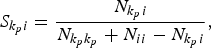 $$S_{k_p i}=\displaystyle{{N_{k_p i} } \over {N_{k_p k_p }+N_{ii} - N_{k_p i} }}\comma \;$$
where k p is subset k composed by subsequent machines of workpiece p; i is a fractal that pursues all machines to manufacture k p; i ∈ {1, … , n c}; N k pi is the number of machines in common between k p and i; N k pk p is the number of requested machines of k p; and N ii is the number of machines of fractal cell i. Make Inter_travel ← 0. For each k p, S k pi is calculated for all available fractal cells i that pursues all machines to manufacture k p. The fractal cell with the highest similarity in comparison to k p is then chosen. Keep it by using a variable last_fractal ← i. Repeat the same calculation for the next k up to K, and the subsequent chosen fractal i″ cell must be different to last_fractal. Update last_fractal ← i″. Based on the information of Step 9 about the distance between fractal cells i and i″, compute Inter_travel ← D i, i ″ + Inter_travel. Repeat the procedure up to K and for all workpieces P.
Step 12.2. In order to reduce the intertravel distance, make Inter_travel ← 0. There are two possibilities for choosing the closest fractal cell:
12.2.1. When k p = 1, then the variable inter_travel remain unchangeable.
12.2.2. When k p > 1, then for k p = 1 verify if all requested machines belong to available fractal cells. Calculate the similarity S k pi and keep the fractal cell that yields the highest value of similarity by using a variable last_fractal ← i. For the next k p, analyze if all requested machines belong to fractal cells. Then based on information provided by Step 9, compare the distance between last_fractal and each available fractal cell i. The fractal cell with the lowest distance, i″, is then chosen. Compute Inter_travel ← D i, i ′ + Inter_travel. Update the variable last_fractal ← i ″. Repeat the procedure up to K. Repeat for all P.
Step 13. Intratravel calculation: we developed a Tabu search heuristics in order to identify the positions of the machines that result in the lowest routing distance for workpiece p during the manufacturing of each k p. The heuristics works in the following way:
Step 13.1. For designated fractal cell i for manufacturing k p, choose randomly requested machines, which are responsible for manufacturing each q k p, and identify its coordinates (x and y).
Step 13.2. Make intra_travel ← 0.
Step 13.3. If q k p = 1, then the variable intra_travel remains unchangeable.
Step 13.4. If q k p > 1, then from q k p = 2 up to k p, calculate the distance Intra_travel ← d + Intra_travel.
Step 13.5. Repeat several times, variable iteration, Steps 13.1 up to 13.4, in order to find the lowest distance in each fractal cell i. In summary, Steps 13.4 and 13.5 may be expressed as shown in Eq. (10):
 $$d=\min \left\{\sum\limits_{q_{k_p }=2}^{Q_{k_p } } {\vert x_{q_{k_p } }^{i_{k_p } } - x_{q_{k_p } - 1}^{i_{k_p } } \vert +\vert y_{q_{k_p } }^{i_{k_p } } - y_{q_{k_p } - 1}^{i_{k_p } } \vert } \right\}\comma \;$$
subject to x, y ∈ integer; x ∈{1..X}; y ∈{1..Y}; i is the chosen fractal cell, defined by Step 12, to manufacture subsequent operations k of workpiece p.
Step 13.6. Repeat Steps 13.1 up to 13.5 for K and then extend it for all workpieces P.
Step 14. Calculate and keep the value of total distance, by using a variable called Total_distance ← Intra_travel + Inter_travel.
Step 15. Calculate the makespan.
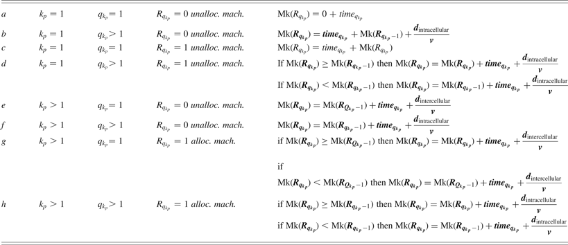
Step 15.1. Calculate the makespan for each workpiece p (see Table 1). The variable d intracellular is the distance of machines responsible for subsequent operations obtained from Step 13.5 and d intercellular is the distance between the current fractal cell i and the selected fractal cell i″, obtained from Step 12. Both variables are used to compute the traveling time. Other times, such as setup time, cleaning time, traveling time from the entrance to machines, and from machines to exit, are omitted. To interpret the information of Table 1, we will analyze only when all machines are unallocated, because the idea for busy machines are quite similar, by using remaining expressions. An unallocated machine means the task had never been allocated to a machine of the best virtual cell of the selected fractal cells. Consider the first workpiece, demanding five operations and separated in two subsets. The first subset (k p = 1) is composed of three operations and the second, k p = 2, of two operations (so Q k p = Q 1 = 3 and Q k p = Q 2 = 2), respectively. To calculate the makespan for this workpiece, because Q 1 >1, use the expression a for the first operation of Q 1 (that is q 1 = 1) and then the expression b for q 1 = 2, q 1 = 3. For the next k p, that is k p = 2 (which is k p > 1), use initially the expression e for the first operation of the second subset (q 2 = 1), and then f for q 2 = 2 (which is q 2 > 1), and so forth. Repeat it for all P.
Calculation of the makespan for each workpiece p submitted to selected fractal cells

Note: Adapted from Chin (Reference Chin2013).
Step 15.2. Compare the makespan of all machines and keep the highest value of makespan (because the manufacturing is concluded only after the last operation has finished).
Step 16. By using a variable named changing_positions, reorder the positions of the machines that belong to each fractal cell, changing_positions times from Step 11 up to Step 15.2. For each iteration of the variable changing_positions, compare the calculated Total_distance and keep the lowest distance and its respective makespan.
4. CASE STUDY
4.1. Layout and workpieces features
This section presents layout and workpiece features, which both are submitted to simulation. It is important to remember that according to Venkatadri et al. (Reference Venkatadri, Rardin and Montreuil1997), the number of fractal cells can be estimated by dividing the total number of machines by the types of machines. This result also defines the number of possibilities about how each fractal cell can be allocated on the shop floor. Taking this information to account (number of fractal cells), for the simulation, we have chosen three sizes (small, medium, and large sizes) of layouts in order to increment, in a purpose way, the number of fractal cells.
First, there are 5 types of machines, resulting in a total of 16 machines, such as used in Benjaafar and Sheikhzadeh (Reference Benjaafar and Sheikhzadeh2000). Thus, there are (16/5) ≈ 4! possibilities for allocating fractal cells. All these machines form X = 4 and Y = 4. Each type of operation process and their respective replicas are the following:
• operation process 1: 1 replica of a machine
• operation process 2: 2 replicas
• operation process 3: 3 replicas
• operation process 4: 5 replicas
• operation process 5: 5 replicas
Second, in order to increment the number of fractal cells, in this research we remained with 5 types of machines forming a layout size 30, which means 30 machines (with configuration X = 5 and Y = 6). Thus, for this case, there are 30/5 ≈ 7! possibilities. Replicas of each type of machine are the following:
• operation process 1: 1 replica of a machine
• operation process 2: 4 replicas
• operation process 3: 7 replicas
• operation process 4: 8 replicas
• operation process 5: 10 replicas
A reference to consider a layout as large size can be seen in Narayanan (Reference Narayanan2007), when it was considered 100 machines. In our research paper, we adopted a total of 120 machines with configuration X = 10 and Y = 12, composed by 8 types of machines (resulting in 120/8 = 16! possibilities). Replicas of each type of machine are shown below:
• operation process 1: 4 replicas of a machine
• operation process 2: 8 replicas
• operation process 3: 10 replicas
• operation process 4: 14 replicas
• operation process 5: 17 replicas
• operation process 6: 19 replicas
• operation process 7: 22 replicas
• operation process 8: 25 replicas
We generated 100 different workpieces, but only 40 of them are randomly selected (workpieces may be repeated). Each one demands from n(i) = 1 up to n(i) = five operations, and requested machines by subsequent operations are different. Because the type of requested machines is proportionate to the number of replicas of machines, we adapt and implement the Monte Carlo simulation based procedure proposed by Chin (Reference Chin2013) for generation of workpieces.
The time taken by each operation varies from 30 to 150 units of time.
We modeled and simulated all of the previously cited features in the following hardware settings: 2-GHz Pentium(R) Dual-Core CPU, 4 MB DDR2 RAM, and platform Pascal programming.
4.2. Definition of input parameter for simulating fractal layouts
In order to obtain simulation results of fractal layouts (traveling distance and makespan), some parameters must be defined, such as max_diff, Tabu_allocation_cells, k, iteration, changing_positions, and v. In the following, the meaning and the adopted value for each variable will be described.
In this research paper, the order of how fractal cells are chosen and allocated is considered. The allocation is based on the difference of similarity (max_diff), which means segregation and allocation of fractal cells is based on similarities. For instance, let us consider a value 0.5 for the variable. If the calculated similarity of a certain fractal cell is located between 1 and 0.5, then it is grouped with others fractal cells located in this same interval and allocated as far as possible to each other. Considering a value closer to 1, then all machines tend to form one only fractal cell, and in this case, intertravels tend to be eliminated and only intratravels occur. In summary, a fractal layout tends to perform similarly to a distributed layout when max_diff is closer to 1. For the evaluation of influence of interval on the performance, we choose values located between 1 and 0. Thus, we established four different values, which are 0.1, 0.3, 0.5, and 0.7.
For the variable Tabu_allocation_cells, we adopt a large enough value (10,000; see Appendix A). The computational model developed, then, calculates the distribution degree for each allocation. Repeat the allocation of cells Tabu_allocation_cells times (i.e., 10,000), which means the distribution degree calculation is also repeated 10,000 times. The allocation of the fractal cell that yielded the lowest value of the distribution degree is then retained. The result is similar for fractal cells as far as possible.
Once each fractal is allocated, now we need to define how workpieces are submitted to fractal cells. The decision of how workpieces will be submitted to fractal cells depends directly on the replica of each type of machine. That is, because of inequality of replicas of each type of machine, some fractal cell may pursue a specific type of machine, making necessarily a certain workpiece to travel between fractal cells. Thus, in order to simulate intertravel, in this research paper we adopt the division of operations to subsequent operations, represented by the variable k. For instance, if possible values of k are between 2 and 5, this means that operations of each workpiece can be separated into two to five parts, and each k is totally processed in the chosen fractal cell. Because we considered (as data input) up to n(i) = 5 operations for each workpiece, the maximum value to be attributed to k is 5, that is, 5 sets where each set is composed of one operation. Therefore, when k = 2 or k = 3, this does not mean that operations of all workpieces will be necessarily separated into two or three sets of workpieces, because the separation depends on the number of operations.
In order to process the first k of each workpiece, the fractal cell must be chosen. The paper is based on the comparison of the similarity between requested machines of each k and machines of each fractal cell. The fractal cell that pursues the highest similarity is chosen. Once k of a certain workpiece is processed in the chosen fractal cell, we need to define how to process k p+1. Thus, here we considered two approaches: based on the similarity and based on the closest distance. This proposed method analyzes all possible available fractal cells (by comparing requested machines of k p + 1 to machines of each fractal cell i′), compares the distances of each one, and selects the closest one (now called i″) in relation to i. After this, the processed workpiece leaves a fractal cell i and reaches i″.
The identification of a virtual cell in a fractal cell to process a certain k is searched iteration times (through the use of the developed Tabu search algorithm procedure). For the variable iteration, we adopt 500 (see Appendix A). That is, the developed computational software is designated to search 500 times the set of machines (remaining the lowest distance) for each k workpiece.
We also need to define a value for the variable changing_positions (see Appendix A). This determines the number of changing positions of machines in order to form new virtual cells in each fractal cell. For instance, if changing_positions receives a value 10, this means the procedure of randomly selection and reallocation of machines is repeated 10 times for each ith fractal cell, resulting in new virtual cells. Although variables iteration and changing_position are associated with intracellular traveling distance calculation, there is an objective function of minimization only for the first one. Thus, for the second, we simply adopt a value higher than 30 (here we adopt variable changing_positions equal to 10,000) just because of statistics issues.
Finally, for the variable v (which represents the workpiece routing velocity), we could test high and low velocities. For the first situation, the traveling time becomes insignificant in comparison to the makespan. Thus, it might be omitted. To avoid it, we decide to adopt a reduced velocity (a constant value of 0.5 units of distance per units of time).
The computational results are organized as follows: by layout size 16 (X = 4 and Y = 4), 30 (X = 5 and Y = 6), and 120 (X = 10 and Y = 12) of machines; by variable called max_diff; by balanced or unbalanced quantity of machines between fractal cells; and by k. We adopted only k = 1, k = 2, and k = 3; and choose next fractal cell i″ to process the next k based on the highest similarity and the closest distance.
For each layout size, 30 samples of input (each one composed of 40 workpieces) are generated. For each submitted sample, there is one best layout because machines of each fractal cell are allowed to change the position (affecting therefore the virtual cell formation). After submitting these 30 samples to the computational model (hence, there are 30 best layouts), two performance parameters (the means and standard deviation of the total distance and of the makespan) are calculated, which are given in units of distance and units of time, respectively. Independent of the layout size, by submitting 30 samples to the computational model, the CPU takes around 5 min 8 s to obtain these two performance parameters, and the CPU time for segregating and allocating fractal cells on the shop floor demands lower than 1 s.
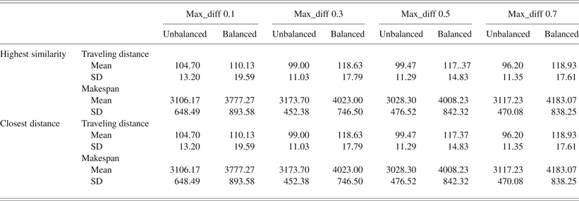
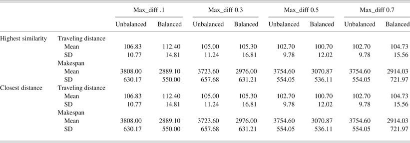
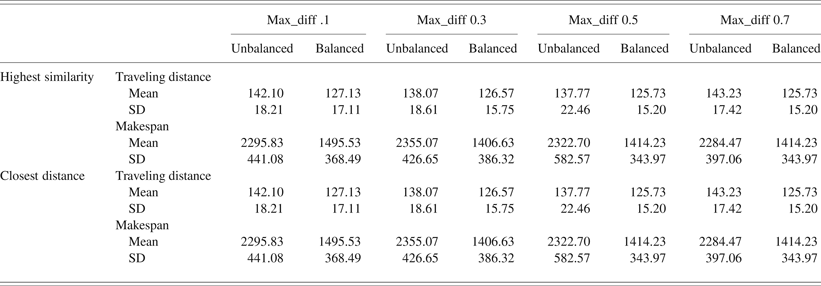
Because intercell traveling is undesirable, we consider k = 1, meaning that all operations of each workpiece are totally manufactured by machines located in the chosen fractal cell. Table 2 presents results, in total traveling distance and the makespan of the layout composed of 16 machines. Results are shown in Table 3 for layout composed of 30 machines. Finally, the performance of the layout size 120 machines can be seen in Table 4. Thus, these three tables demanded 4 h 6 min 36 s of CPU time.
Layout with 16 machines (4 × 4)
Layout with 30 machines (5 × 6)
Layout with 120 machines (10 × 12)
Table 2 shows that when k = 1, segregating and allocating as far as possible similar fractal cells (represented by the variable max_diff) and choosing the next fractal cell based on any adopted criteria (represented by the highest similarity and the closest distance) for manufacturing the next k do not affect the performance. Only the balanced and unbalanced quantity of machines forming each fractal cell affects the performance. In addition, based on our results, the unbalanced quantity of machines performs better in comparison to balanced quantity of machines, because both parameters are concomitantly reduced (balanced: around 115.00 of traveling distance, in units of distance, and around 4000.00 of makespan, in units of time; unbalanced: around 99.00 of total traveling distance, in units of distance, and 3100.00 of makespan, in units of time). In short, there are reductions of 13.91% in total traveling distance and 22.50% in makespan.
Increasing the total number of machines, from 16 to 30, the performance parameters still are affected only by the balanced and unbalanced quantity of machines. Note that, this time, the performance yielded (in total traveling distance), by applying balanced quantity of machines, became similar to the unbalanced quantity of machines (see Table 3). It is surprising that the makespan becomes lower (unbalanced: around 3700.00; balanced: 2900.00), with a reduction of 21.62%.
In the layout size composed of 120 machines, the performance parameters of fractal cells, composed of a similar quantity of machines (balanced quantity of machines), resulted in a reduction of the total traveling distance and makespan (around 10% and 38.26%, respectively) in comparison to the unbalanced quantity of machines (see Table 4).
4.3. Performance comparison among fractal layout, distributed layout, and functional layout
This section introduces the performance among the fractal layout, the distributed layout, and the functional layout. There are three well-known types of distributed layout: randomly distributed layout, where types of machines are randomly selected and allocated on the shop floor; partially distributed layout, where groups of the same type of machine are formed and allocated, and maximally distributed layout. For partially distributed layout, disaggregation is considered. For instance, if there is one level of disaggregation, it means there are two groups of the same type of the machine allocated on the shop floor. Initially proposed by Francis and White (Reference Francis and White1974), a measure (distribution degree) is used that aims to maximize the allocation position of the same type of machine on the shop floor. The layout that pursues the lowest distribution degree is maintained and then the maximally distributed layout is finally obtained.
Thus, beyond the fractal layout model, we construct the computational models in order to generate distributed layouts, functional layouts, and also another model to simulate the performance, by submitting the same workpiece's features.
The adopted procedure to generate each type of distributed layout did not take into account flow material but only replicas of each type of machine, such as used by Benjaafar and Sheikhzadeh (Reference Benjaafar and Sheikhzadeh2000). For partially distributed layout, we adopt two levels of disaggregation.
The procedure for generating functional layout consisted in defining the SFC (in this research paper, we adopt the simplest one; see Sagan, Reference Sagan1991)). Next, a machine is randomly selected and allocated on the shop floor. The allocation continues until the replica becomes zero. When it occurs, the next type of machine is selected, and so forth, until all types of machines are allocated.
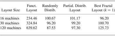
For these two types of layouts, there are 30 samples of each one. Hence, in functional layout, for 16 machines, there are 30 samples of layouts. In functional layout, for 30 machines, there are others 30 samples of layout,s and so forth. For each sample, we submitted 30 samples of parts (each one composed of 40 workpieces). The average of the mean of the traveling distance can be seen in Table 5.
Average of the mean of the total traveling distance (units of distance)
In Table 5, notice that in relation to total traveling distance, the performances of distributed layouts and fractal layout for small to medium size are similar. These performances were expected because in fractal layout only intracellular traveling distance will be computed (when k = 1). In short, a fractal layout tends to perform similarly to a distributed layout. For our large layout size, randomly distributed layout presents better performance in traveling distance in comparison to fractal layout. It was expected that the functional layout presents the worst performance in comparison to distributed layouts because of interdepartmental trips. Due to the worst performance of the functional layout, its makespan will not be computed.
Next, we compare the best of the functional layout, the best of distributed layout (maximally distributed layout), and the best of the fractal layout (when k = 1).
It is important to remember that, in fractal layout, there are not 30 samples of fractal layouts. That is, there is 1 best for each submitted sample of workpieces. Thus, in order to conduct the same comparison, we need to work with only 1 sample of layout and 30 samples of workpieces (which is composed of 40 workpieces).
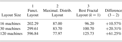
In the functional layout, after submitting 40 workpieces, the computational model exchanges the position of each department and keeps the lowest total traveling distance. For the exchange step, we need to adopt a higher enough value (we adopted also 10,000). Submit other samples (up to 30) and repeat the exchange procedure. The results (mean of the lowest traveling distance) are provided in Table 6. Note the performance of thefunctional layout has improved. Nevertheless, it is still the worst.
Mean of the total traveling distance (units of distance)
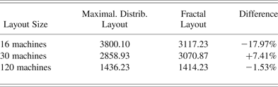
In the maximally distributed layout, there is no exchange because machines are already in the best positions. Thus, after submitting 30 samples of workpieces, the results (mean of the traveling distance) can be seen in Table 6. Comparing the maximally distributed layout to the fractal layout, in general, the first presents higher performance (better). The fractal layout outperforms the maximally distributed layout only in terms of makespan for the small size of the layout (–17.97%; see Table 7). For the large size (120 machines), the total traveling distance and the corresponding makespan of the fractal layout (+61.25%, see Table 6; –1.53%, see Table 7) are in comparison to the maximally distributed layout.
Mean of the correspondent makespan (units of time)
Based on our results, the maximally distributed layout seems to satisfy concomitantly the two adopted performance parameters (total traveling distance and makespan), except for the small layout size. However, as pointed out by Benjaafar and Sheikhzadeh (Reference Benjaafar and Sheikhzadeh2000) and Askin et al. (Reference Askin, Ciarello and Lundgren1999), in order to implement a suitably distributed layout, an efficient control system is required for identifying available machines to form efficient virtual cells, which naturally implies a high cost for the implementation. An alternative to minimize the cost of implementation is to segregate machines to form groups of it, where technology can be shared between machines.
As shown in previous sections, in the fractal layout, there are two possibilities: when k = 1, for which the workpieces are totally manufactured in a fractal cell; and k > 1, when intercellular travel occurs. Because of different replicas of each type of machine, we simulate intertravels by adopting k > 1 (k = 2 and k = 3), as shown in next section.
4.4. Simulation of intercellular travels in fractal layouts for k > 1
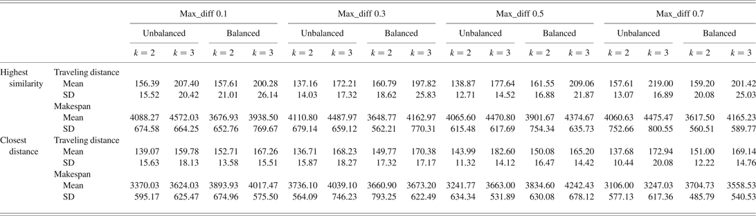
This section aims to analyze results of intertravels (when k >1) in fractal layouts obtained from the developed computational simulation model. We show the total traveling distance and its respective makespan to three adopted layout sizes (i.e., 16, 30, and 120 machines; see Tables 8–10).
Layout with 16 machines (4 × 4)
Layout with 30 machines (5 × 6)
Layout with 120 machines (10 × 12)
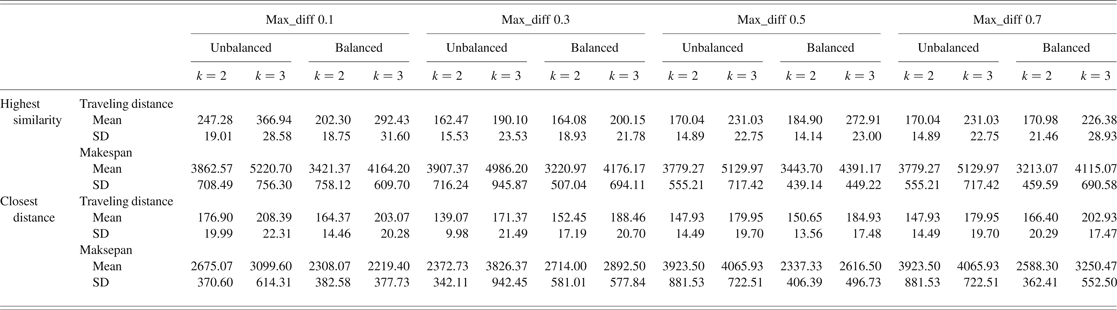
We notice that once intercellular traveling distance increases, the total traveling distance increases significantly. The mathematical proof is in Appendix B, and it proves our constructed computational model is valid. Moreover, it shows any tentative prediction for the minimization of intercellular traveling distance is appreciated. In order to discriminate the intercellular traveling distance from total traveling distance, we constructed Figures 1– 5. Figure 1 presents the performance of the intertraveling distance of submitted workpieces to the layout composed by 16 machines, and Figure 2 show the corresponding makespan.
The layout with 16 machines (4 × 4).
The layout with 16 machines (4 × 4).
It is already expected that the intercellular traveling distance becomes zero when k = 1 because the operations are totally executed in the fractal cell previously selected. Due to different replicas of each type of machine, the intertravel occurs, so we need to simulate it by adopting different short values for k (k > 1). We adopted k = 2 and k = 3, which means operations of a certain workpiece p can be separated up to two or three sets.
We will start the analysis when a fractal cell is chosen based on the highest similarity criteria selected. Comparing results, when k = 2, the intercellular traveling distance may be reduced by adopting and unbalanced quantity of machines and adopting a value of max_diff equal to 0.3. For this input parameter, we obtained an intercellular traveling distance of approximately 80 units of distance and a makespan of 4100 units of time. When k = 3, we obtained an intercellular travelling distance of 140 units of distance and a makespan of 4500 units of time. In addition, observe that minimization of intercellular trips does not imply in makespan minimization (see Figure 2).
The best result is reached when we adopt: unbalanced quantity of machine, the closest fractal cell chosen, and max_diff equal to 0.1. Although there are cases with a trade-off behavior, it is possible to minimize both parameters (intercellular travelling distance and makespan).
It may be generally concluded that, at this layout size, choosing a fractal cell based on the closest distance criteria yields a lower mean of the intercellular traveling distance in comparison to the highest similarity criteria. In addition to this fractal cell choice circumstance, when an unbalanced quantity of machines is adopted to form each fractal cell, it yields the lowest mean of the makespans. Figure 3 shows the performance of the intercellular traveling distance for the layout composed of 30 machines.
The layout with 30 machines (5 × 6).
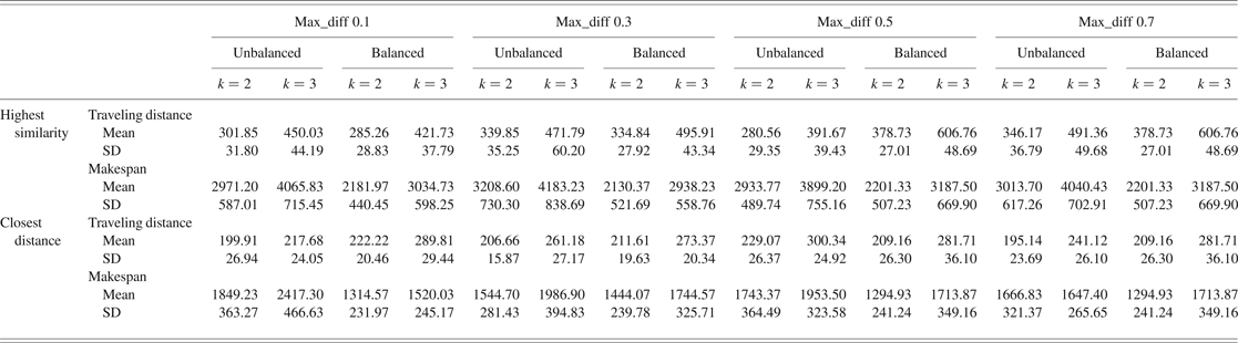
Thus, even when k = 1, it is expected that the intertravel distance becomes zero. For k > 1, a different performance of intercellular traveling distance can be obtained by varying values of the variable max_diff (represented by similarity 0.1, 0.3, 0.5, and 0.7). It is noticed that the lowest mean value of the intercellular traveling distance is reached when we adopt a value of 0.3 to max_diff variable and an unbalanced quantity of machines to form each fractal cell, and choose the closest fractal cell to manufacture the next k. These parameters yield a reduced mean of the intercellular traveling distance (around 75 units of distance; see Figure 3) and a corresponding makespan value (~2300 units of time; see Figure 4). Analyzing Figure 4, there is another makespan value closer to 2300 (for k = 2, max_diff = 0.1, balanced quantity of machines, and closest fractal cell), but the mean of the intercellular traveling distance receives an increment to around 35 units of distance. For k = 3, the lowest average traveling distance is obtained for max_diff equal to 0.3, unbalanced quantity of machines, and the closest fractal cell. Nevertheless, there are other reduced values of makespans, such as by adopting max_diff equal to 0.1, unbalanced quantity of machines, and the closest fractal cell.
The layout with 30 machines (5 × 6).
Finally, the results of 120 machines can be seen in Figure 5 and Figure 6. In short, for k = 2, the closest distance criteria outperforms in comparison to the highest similarity criteria. It can be confirmed in Figure 5, in which for any value of the variable max_diff, there are reduced average values of intercellular traveling distances (around 135 units of distance).
The layout with 120 machines (10 × 12).
The layout with 120 machines (10 × 12).
Moreover, for k = 2, even max_diff equal to 0.1 or equal to 0.7 might be used (in addition to the closest distance criteria and unbalanced quantity of machines) because both yields have reduced the intercellular traveling distance (~125 units of distance). Nevertheless, regarding makespan, max_diff equal to 0.1 yields higher makespan than max_diff equal to 0.7. When k = 3, max_diff equal to 0.1 yields the lowest average intercellular traveling distance (when the closest distance and unbalanced quantity of machines are adopted). However, the makespan becomes higher than other max_diff values.
4.5. Comparison between the literature (no similarity) and the best result of our proposed method
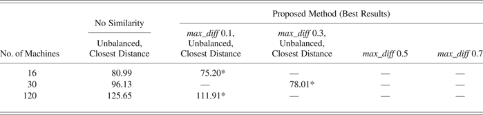
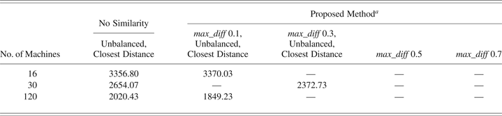
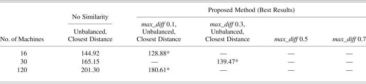
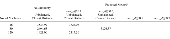
Tables 11, 12, 13, and 14 show the performance in intercellular traveling distance and makespan to three adopted sizes of layout. Concerning the relevant proposed method, only the best results are shown. Note that best results are obtained when the unbalanced and the closest distance strategies are adopted. Aiming to simulate the performance of fractal layout without considering segregated fractal cells based on their similarities, we adopted a reduced value of max_diff, particularly equal to 0.05, which means reduced segregated fractal cells (or no similarity). To keep the same comparison base, we use the same parameters to simulate the performance (unbalanced and the closest distance strategies). For more details, see Appendix C.
Mean of the intercellular traveling distance (for k = 2)
Mean of the correspondent makespan (for k = 2)
aCorrespondent makespan associated with Table 11.
Mean of the intertraveling distance (for k = 3)
Mean of the correspondent makespan (for k = 3)
aCorrespondent makespan associated with Table 13.
For k = 2, the best result yielded by adopting with no similarity, considering 16 machines, was 80.99 units of intercellular traveling distance, and for this proposed method, 75.20, which means a reduction of 7.15%. Considering 30 machines, the reduction becomes 18.85%, and for 120 machines, the reduction becomes 10.94%. Thus, when k = 3 is adopted, our proposed method yields a reduction of 11.07% for 16 machines, a reduction of 29.09% for 30 machines, and a reduction of 10.28% for 120 machines.
We notice in Tables 11 and 13 after 5 min 8 s, the simulated traditional fractal layout still could not find the best allocations for fractal cells. In contrast, for the same consumed CPU time, based on our proposed criterion (represented by max_diff), better results are obtained. Specifically, in less than 1 s of the total consumed CPU time (5 min 8 s), the computer could reach the “quasi” optimal allocation.
Based on all presented results, we may affirm an unbalanced quantity of machines strategy produces better results than a balanced quantity of machines. Likewise, in around 66.67% of our cases studies (see Tables 11 and 13) decreased values for the variable max_diff are desired (specifically, 0.1).
Although it may be possible to reach better results by executing several times the procedures for the allocations of the fractal cells and the flow assignments (as proposed in the literature and represented in our research work by “no similarity”), it is expected at higher consumed CPU time. Figure 7 shows the relation between mean of the intercellular traveling distance and iteration (number of changing positions of fractal cells based on the literature procedure). When the iteration is 5 means, the fractal cells changing positions are executed 5 times for each submitted sample of workpieces, retaining the lowest intercellular traveling distance, and repeating for all others 29 samples of workpieces. Thus, the presented intracellular traveling distance is, actually, the mean of these 30 samples. Because the allocation of fractal cells is randomly executed, it does not mean necessarily the minimization of the mean of the intercellular traveling distance, so it helps to explain why in a few cases high/low values are observed of intercellular traveling distance as iteration increases. Note that with increasing the number of iterations, the CPU times increase significantly.
The relation between the mean of the intercellular traveling distance × the iteration.
We also note the increasing of the number of iterations; the result of “no similarity” becomes similar to our proposed method (compare to Tables 11 and 13). Nevertheless, in some cases, there is no need to execute several times the allocation of fractal cells because the results are quite similar to our proposed method. For instance, when k = 2, reduced values of iterations are required. When k = 3, the proposed procedure tends to increase the effectiveness of allocations of fractal cells.
5. CONCLUDING REMARKS
This section provides conclusions about the results obtained from the constructed computational simulation model.
Based on the reviewed articles, proposed procedures are used several times to execute the allocations of the fractal cells and the flow assignment, both concomitantly, in order to find the best one. As pointed out by Montreuil et al. (Reference Montreuil, Venkatadri and Rardin1999), depending on the number of estimated fractal cells, the number of possibilities for allocating it on the floor may increase significantly, which may demand huge computational time. Thus, it is important to define a procedure spreading fractal cells on the shop floor efficiently. In this research paper, we propose a fractal cells similarity-based criterion, which consists in segregating similar fractal cells according to the movable intervals. Only after the definition of best allocation of the fractal cells, the flow assignment occurs. The procedure appears to be quite promising because it demanded reduced computational effort (<1 s).
Naturally, the best strategy is k = 1 in which no intercells trip occurs. For this case, it is suggested that maximally distributed layout be implemented, especially for large size of layout, in which makespan and total traveling distance are minimized. Owing to unequal replicas of machines and other issues, such as sharing technologies for an efficient production controlling system, intercellular trips happen inevitably.
It is assumed that adopting the strategy by choosing fractal cell to manufacture next k based on highest similarity, the makespan might be reduced compared to the strategy by choosing the closest fractal cell criterion. However it does not happen.
In general, it may be concluded that adopting the closest fractal cell criterion to manufacture the next k results in lower average of the intercellular traveling distance than the highest similarity criterion. Although the minimization of intercellular traveling distance has been explored in the literature, it does not mean the minimization of makespan. In many cases, based on our experiments, there is a trade-off behavior, that is, when the average of the intercellular traveling distance is reduced, the average of the makespan is increased, or vice versa. Thus, it is important, if possible, to minimize concomitantly makespan and intercellular traveling distance by identifying the best settings, such as for 30 machines: unbalanced quantity of machine, k = 2, choosing the closest fractal cell, and similarity equal to 0.3.
Based on our research, we notice that the quantity of machines to form each fractal cell is an important parameter to be considered, because it affects directly the performance of the production systems. Besides, it shows that in most cases low value to variable max_diff is required.
As a suggestion for future studies, other values of k and other values for the variable max_diff might be tested in order to complement what we have presented in this research paper. Chin (Reference Chin2013) and Gorgulho Júnior and Gonçalves Filho (Reference Gorgulho Júnior and Gonçalves Filho2007) have pointed out the importance in evaluating the performance of production systems when workpieces may be obtained in many ways (i.e., it does not follow only one operation sequence).
In addition, other values for variables Tabu_allocation_cells, iteration, and changing_positions could be tested. It is expected the that performance of fractal layouts would be improved.
In this paper, we implemented a simple SFC. Based on the results, we may affirm the intracellular traveling distance does not really affect the performance of the total traveling distance. Nevertheless, other SFCs could be tested (see Sagan, Reference Sagan1991).
6. LIST OF ABBREVIATIONS
- d
distance between machines responsible for processing subsequent operations of each k
- D
distance between two fractal cells computed from the centroid of each one
- g
gth fractal cell G
- G
fractal cells grouped in the same movable interval G
- i
ith fractal cell
- i′
ith fractal cell
- i″
next chosen fractal cell
- j
jth operation of workpiece p
- k
kth subset of operations of a certain workpiece
- K
total number of subsets of operations of a certain workpiece p
- minmax
minimize the maximum distance of different types of machines
- Mk(R q k)
makespan of machine responsible for processing the q kth operation
- n c
number of fractal cells
- p
pth workpiece
- P
total number of parts
- q k
q kth operation of kth subset
- Q k
total number of operations of kth subset
- R q k
replica of machine responsible for processing q kth operation
- time q k p
time of q k pth operation of k p subset
- x q ki k
horizontal coordinate of the machine, belongs to the ith fractal cell, which is responsible for the q k operation
- x q ki k
vertical coordinate of machine, belongs to the ith fractal cell, which is responsible for the q k operation
- x ki k
horizontal coordinate of the centroid of fractal cell i, which is chosen for processing subset k
- y ki k
vertical coordinate of the centroid of fractal cell i, which is chosen for processing subset k
- X, Y
horizontal and vertical coordinates of the layout
- v
workpiece routing velocity
ACKNOWLEDGMENTS
The authors acknowledge three anonymous reviewers for valuable comments and suggestions that contributed significantly to the improvement of this research work.
Yung Chin Shih is a Professor at the Technological Federal University of Paraná, where he teaches subjects such as queueing theory, quality control, logistics, production planning and control, facilities planning, and computational modeling and simulation. He serves as a referee for several international journals and has authored numerous articles. His research interests are in developing bioinspired algorithms for improving the performance of warehousing and manufacturing systems.
Eduardo Vila Gonçalves Filho is currently a Professor at the University of São Paulo. He attained a PhD in industrial engineering from Pennsylvania State University in 1988. Dr. Gonçalves Filho has experience in production engineering, with emphasis on planning, design, and control of production systems. Other areas of interest are product design, design for manufacturing, and assembly and manufacturing processes. He has acted as a referee for several journals and is the author of numerous articles.
APPENDIX A
A.1. Analysis of suitability of adopted values for the variables associated with loops
According to the order of the article, there are three types of loops. The first is associated with the allocation of fractal cells on the shop floor (Tabu_allocated_cells), which affects directly the intercellular traveling distance, see Proof 1. The second is associated with the identification of virtual cells (iteration), and the last one is associated with changing positions of machines (changing_positions) in a fractal cell. These last two affect the intracellular traveling distance, so both will be analyzed in Proof 2.
Proof 1: Analyzing the variable used for the calculation of intercellular traveling distance. After the segregation procedure, we have a typical problem of permutation with repetition. Depending on the number of groups formed by the movable interval, it still may result in a high number of allocation possibilities. We need an alternative for efficient allocation of these groups. ■
We propose here to use the adapted version of the distribution degree [Eq. (A.1)] first proposed by Benjaafar and Sheikhzadeh (Reference Benjaafar and Sheikhzadeh2000):
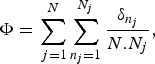 $$\Phi=\sum\limits_{\,j=1}^N {\sum\limits_{n_j=1}^{N_j } {\displaystyle{{{\rm\delta}_{n_j } } \over {N.N_j }}} }\comma \;$$
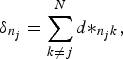 $${\rm\delta}_{n_j }=\sum\limits_{k \ne j}^N {d{\ast}_{n_j k}}\comma \;$$
where d*n jk is the distance between the nth machine of type j and the closest machine type k, n j is the nth machine of type j, N j is the number of machines of type j, and N is the types of machines (departments).
The strategy proposed by the calculation of the distribution degree is to identify replicas of the same type of machine and then allocate them as far as possible. As the distribution degree (given in units of distance) decreases, the best is the spread of the same type of machine.
The calculation of the distribution degree initially ignores the flow assignment. It is concerned with minimizing the average distance among different types of machines. Thus, it is expected to obtain the reduction of the total traveling distance, which occurs only after obtained lowest distribution degree and next calculation of traveling distance through the flow assignment. It helps to explain why a reduced CPU time is observed.
It is also important to observe, when the calculation of distribution degree is done for single replica of different types of machines, independent of how the allocation of machines is realized, the distribution degree is the same as the iteration increases (see an example shown in Figure A.1). This property is valid for any layout size and any types of machines.
The relationship between iterations and the calculated distribution degree for a single machine. Features: format 2 × 4, eight types of machines, one replica of each one.
When replicas of each type of machine increase, the distribution degree tends to decrease, which means the average distance of different types of machines becomes lower. Thus, it is expected reduction of traveling distance among different types of machines (see Fig. A.2)
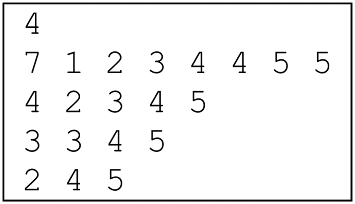
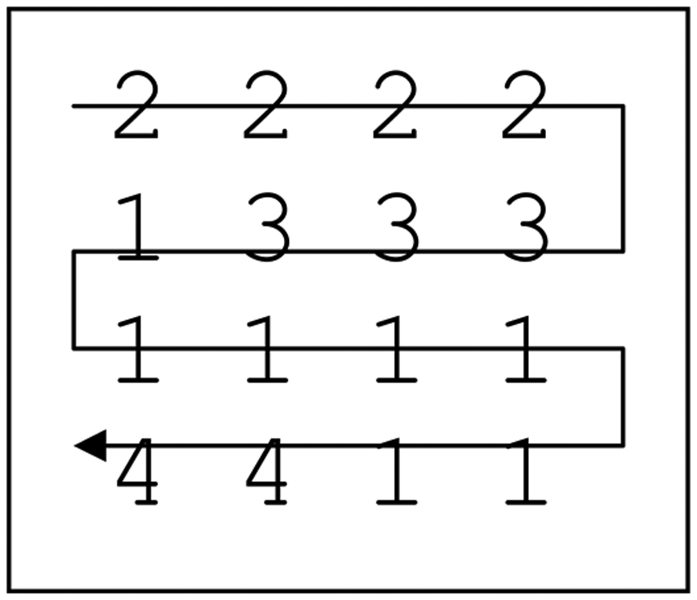
The relationship between iterations and the calculated distribution degree for replicas of machines. Features: format 3 × 4, 8 types of machines, 1 1 1 1 2 2 2 2 (which means 1 replica for machine type 1, 1 replica for machine type 2, etc., totaling 12 machines).
.
For the example shown in Figures A.1 and A.2, we notice if the adopted number of iterations is 2000 for the calculation of distribution degree, no reduction of it is observed.
Our calculation of the distribution degree was applied for the distributed layout. The previous representation of a machine in the distributed layout is now represented by a fractal cell in the fractal layout, and replicas of machines are a set of fractal cells that belong to the same movable interval.
For fractal layouts, even with the same distribution degree, as iterations increase (especially for single replica of machine, which means one movable interval composed by only one fractal cell), it is possible to reduce total traveling distance through flow assignment, because each different fractal cell may be composed of similar machines. In contrast, if fractal cells execute different operations, no reduction of total traveling distance is expected.
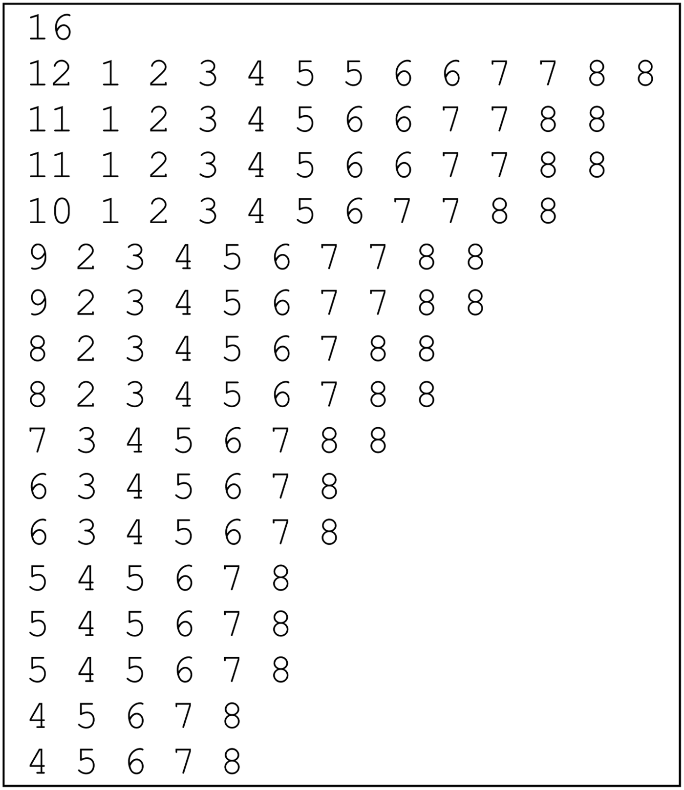
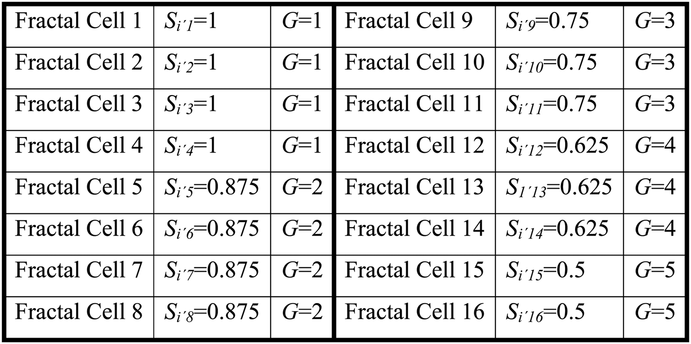
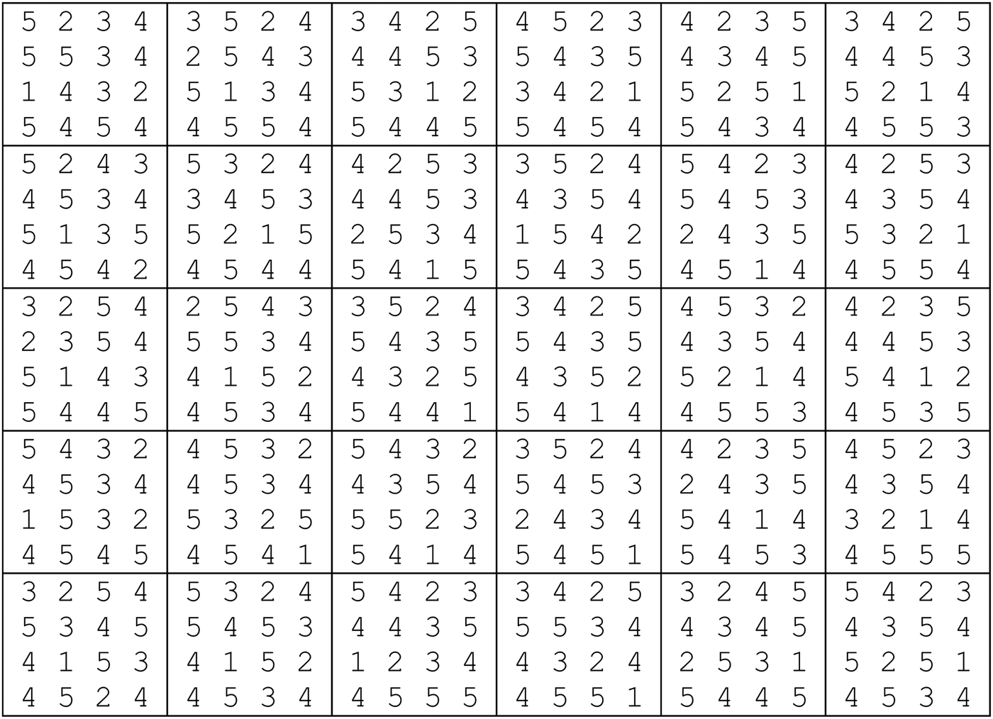
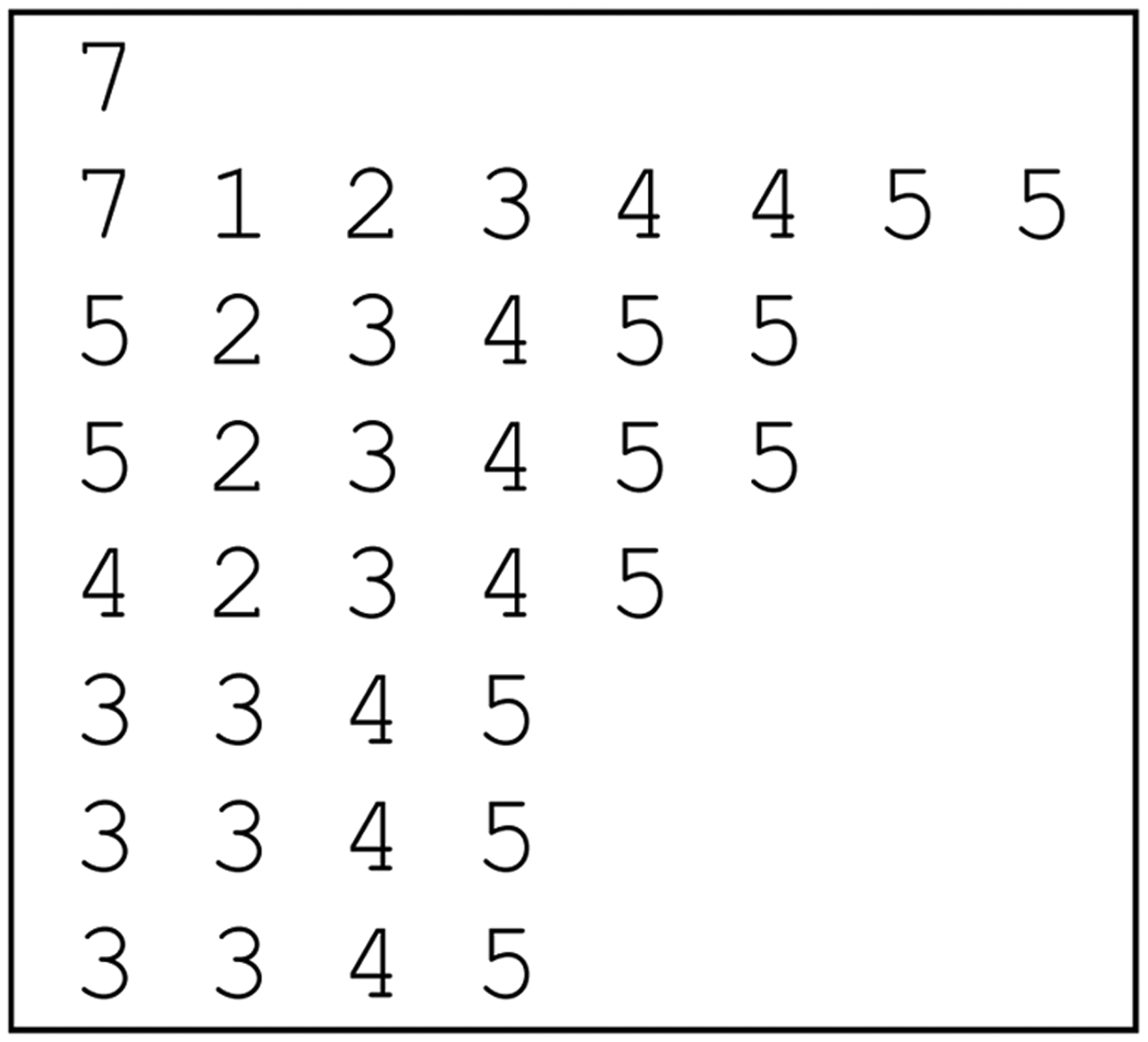
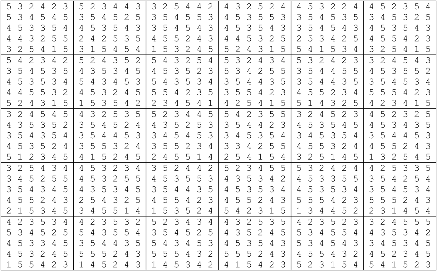
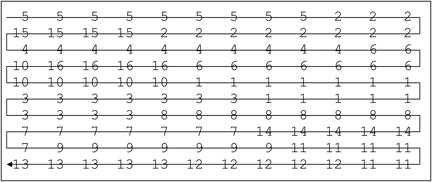
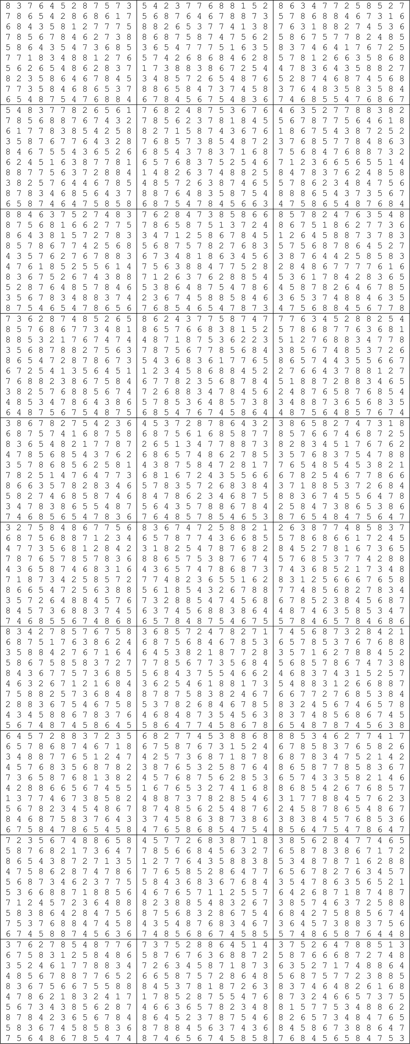
There are several simulation conditions in this research work. To simplify, we will show for the worst case when there is a high number of fractal cells. That is, because once the adopted number of iterations (Tabu_allocated_cells = 10,000) is attended for the worst case, the fractal layout with a small number of fractal cells will be also satisfied. Based on Figure A.3, there are a total of 16 fractal cells. Based on our proposed procedure for the definition of number of intervals, the variable number_intervals is determined, which is equal to 11 ((1/0.1) + 1). In Figure A.4, the first column repeats the information of Figure A.3. The second column shows the calculation of the similarity between the fractal cell and the fractal that pursues all types of machines i′. The third column shows the received G by comparing the calculated S i ′ i to the formed movable interval.
There are a total of 16 fractal cells.
The results after the segregation.
After renaming all machines of each fractal cell by the respective G, the procedure for the calculation of distribution degree starts. The relation between iterations and the distribution degree is shown in Figure A.5. Note that no reduction of distribution degree is observed from the iteration 1500. Consequently, the adopted number of iterations equal to 10,000 is adequate.
The relation between the iteration and distribution degree.
From Figure A.3, we obtained a total number of 16 fractal cells. Thus, by the traditional method, there are 16! possibilities. As shown in Figure 7, after only 80 iterations (of a total of 16!), which is significant lower in comparison to 10,000 adopted for our proposed method, the CPU already consumed 6 h 20 min 24 s. It shows clearly how disadvantage is by the traditional method.
Proof 2: Analyzing the variables used for the calculation of intracellular traveling distance. In the chosen fractal cell i″, where a certain Q k will be processed, the identification of a virtual cell (set of machines) is realized. The number of replicas of each type of requested machine constitutes a routing tree, where the number of possibilities (possibilities for virtual cell formation) is given by Eq. (A.3):
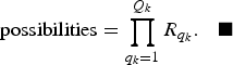 $${\rm possibilities} = \prod\limits_{q_k=1}^{Q_k } {R_{q_k } }.$$
In the presented case studies, the worst case is when there are two replicas of the requested machines. Because the highest value of Q k is 5, it results in 2 × 2 × 2 × 2 × 2 = 32 possibilities for the routing tree. The computational model then calculates, for each one of 32, the distance formed by the machines. The lowest distance is then chosen as virtual cell.
This means that the CPU will need to execute the variable iteration at least 32 times to select the cited virtual cell. Here we adopted 500 (which is oversized), assuming the CPU is capable of selecting all 32 possibilities at least one time.
Figure A.6 shows the evolution of virtual cell formation of 30 samples (each sample composed by 40 workpieces) by the Tabu search heuristics, which is designated to searching the best set of machines. Note that, in most cases, the significant reduction of intratraveling distance occurs up to 500.
The performance of Tabu search heuristics for searching the best virtual cell for the worst case.
From Eq. (A.3), there are two alternatives to increase the number of possibilities (number of operations and replicas of requested machines), which, in theory, would demand more than 500 loops. By keeping other simulation features (inputs) adopted in this research work and increasing the iteration from 500 to 10,000, the consumed CPU time is now 1 h 48 min. Although the CPU time becomes higher (i.e., worsened), the CPU time consumed (traditional method) with this new input is now 149 h 57 min, instead of the previous 6 h 20 min 24 s.
As reported, the variable changing_positions is used to establish the number of times for changing machines' positions, which occurs in a certain fractal cell.
Because the intracellular traveling distance becomes lower in comparison to intercellular traveling distance, see Appendix B, we much concerned with proposing a procedure for fractal cell allocation, instead of proposing a procedure for allocation of machines in each fractal cell. We could also calculate the distribution degree in order to obtain the best spread of the same types of machines as for intercellular traveling distance, but no benefits would bring to reduction of intracellular travelling distance. This is because, using the adopted procedures for separating machines (balanced and unbalanced), it is quite common for each fractal cell to pursue a single machine (not replicated), and as we already proved, the distribution degree tends to be the same. We simply adopt a value higher than 30 just because of statistical issues (changing_positions = 10000).
APPENDIX B
B.1. Relation of magnitude between inter- and intracellular traveling distance
The average distance between fractal cells i and i″ (intercellular traveling distance) can be estimated by Eq. (B.1):
 $$D = \displaystyle{1 \over {N_{i^{\prime \prime} } N_i }}\sum\limits_{i^{\prime \prime} i^{\prime \prime}=1}^{N_{i^{\prime \prime} } } {\sum\limits_{ii=1}^{N_i } {\left\vert {x_{ii} - x_{i^{\prime \prime} i^{\prime \prime} } } \right\vert +\left\vert {y_{ii} - y_{i^{\prime \prime} i^{\prime \prime} } } \right\vert } }\comma \;$$
where x ii, x i ″i ″ represents the horizontal coordinate of the machine that belongs to fractal cells i and i″, respectively; y ii, y i ″i ″ represents the vertical coordinate of the machine that belongs to fractal cells i and i″, respectively; and N i, N i ″i ″ represents the quantity of machines allocated in fractal cells i and i″, respectively.
The average distance between machines in the chosen fractal cell i, machines ii and ii − 1 (intracellular traveling distance) can be estimated by Eq. (B.2):
 $$d_{\rm intracellular \;traveling \;distance} = \displaystyle{{\sum\nolimits_{ii=2}^{N_i } {\left\vert {x_{ii} - x_{ii - 1} } \right\vert +\left\vert {y_{ii} - y_{ii - 1} } \right\vert } } \over {\sum\nolimits_{ii=1}^{N_i } {\lpar N_i - ii\rpar } }}\comma \;$$
where x ii represents the horizontal coordinate of the iith machine that belongs to fractal cell i; y ii represents the vertical coordinate of the iith machine that belongs to fractal cell i; and N i represents the quantity of machines allocated in fractal cell i.
Thus, the possible distances between i and i″ to be computed are the expression in Eq. (B.1) and the intracellular traveling distances before and after reaching i″, which on average is obtained by Eq. (B.3):
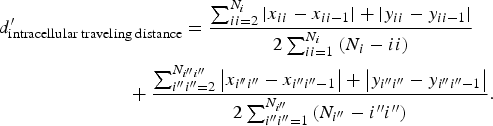 $$\eqalignno{& d_{\rm intracellular \;traveling \;distance} ^{\prime} = \displaystyle{{\sum\nolimits_{ii=2}^{N_i } {\left\vert {x_{ii} - x_{ii - 1} } \right\vert +\left\vert {y_{ii} - y_{ii - 1} } \right\vert } } \over {2\sum\nolimits_{ii=1}^{N_i } {\lpar N_i - ii\rpar } }} \cr &\,\,\;\; \quad\quad\quad\quad\quad\quad +\displaystyle{{\sum\nolimits_{i^{\prime \prime} i^{\prime \prime}=2}^{N_{i^{\prime \prime} i^{\prime \prime} } } {\left\vert {x_{i^{\prime\prime} i^{\prime \prime} } - x_{i^{\prime \prime} i^{\prime \prime} - 1} } \right\vert +\left\vert {y_{i^{\prime \prime} i^{\prime \prime} } - y_{i^{\prime \prime} i^{\prime \prime} - 1} } \right\vert } } \over {2\sum\nolimits_{i^{\prime \prime} i^{\prime \prime}=1}^{N_{i^{\prime \prime} } } {\lpar N_{i^{\prime \prime} } - i^{\prime \prime} i^{\prime \prime} \rpar } }}.}$$
For a given m ∈ {1..n c}, observe the denominator of Eqs. (B.1) and (B.3):
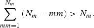 $$\sum\limits_{mm=1}^{N_m } {\lpar N_m - mm\rpar \gt N_m }.$$
Note that there is a trade-off to be analyzed. Thus, we need to prove how disadvantaged one is in comparison to the other.
Renaming the numerators of the expression in Eq. (B.3) as A and B
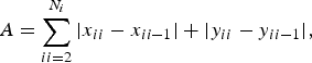 $$A=\sum\limits_{ii=2}^{N_i } {\left\vert {x_{ii} - x_{ii - 1} } \right\vert +\left\vert {y_{ii} - y_{ii - 1} } \right\vert }\comma$$
 $$B=\sum\limits_{i^{\prime \prime} i^{\prime \prime}=2}^{N_{i^{\prime \prime} i^{\prime \prime} } } {\left\vert {x_{i^{\prime \prime} i^{\prime \prime} } - x_{i^{\prime \prime} i^{\prime \prime} - 1} } \right\vert +\left\vert {y_{i^{\prime \prime} i^{\prime \prime} } - y_{i^{\prime \prime} i^{\prime \prime} - 1} } \right\vert }\comma \;$$
which results in Eq. (B.7):
 $$d_{\rm intracellular \;traveling \;distance}^{\prime} = \displaystyle{{A\sum\nolimits_{i^{\prime \prime} i^{\prime \prime}=1}^{N_{i^{\prime \prime} } } {\lpar N_{i^{\prime \prime} } - i^{\prime \prime} i^{\prime \prime} \rpar +B\sum\nolimits_{ii=1}^{N_i } {\lpar N_i - ii\rpar } } } \over {2\lsqb \sum\nolimits_{ii=1}^{N_i } {\lpar N_i - ii\rpar } \rsqb \times \lsqb \sum\nolimits_{i^{\prime \prime} i^{\prime \prime}=1}^{N_{i^{\prime \prime} } } {\lpar N_{i^{\prime \prime} } - i^{\prime \prime} i^{\prime \prime} \rpar } \rsqb }}.$$
From the numerator of Eqs. (B.1) and (B.7), it is valid that
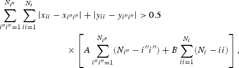 $$\fleqalignno{& \!\sum\limits_{i^{\prime \prime} i^{\prime \prime}=1}^{N_{i^{\prime \prime} } } \sum\limits_{ii=1}^{N_i } \left\vert x_{ii} - x_{i^{\prime \prime} i^{\prime \prime} } \right\vert +\left\vert y_{ii} - y_{i^{\prime \prime} i^{\prime \prime} } \right\vert \gt 0.5\cr &\quad \quad \quad\quad\quad\quad \quad\, \times \left[A\sum\limits_{i^{\prime \prime} i^{\prime \prime}=1}^{N_{i^{\prime \prime} } } \lpar N_{i^{\prime \prime} } - i^{\prime \prime} i^{\prime \prime} \rpar +B\sum\limits_{ii=1}^{N_i } \lpar N_i - ii\rpar \right]\comma}$$
and from (B.4)
 $$\quad \quad \quad \quad\ \left[N_i N_{i^{\prime \prime} }\lt \sum\limits_{ii=1}^{N_i } {\lpar N_i - ii\rpar } \right] \times \left[ \sum\limits_{i^{\prime \prime} i^{\prime \prime}=1}^{N_{i^{\prime \prime} } } {\lpar N_{i^{\prime \prime} } - i^{\prime \prime} i^{\prime \prime} \rpar }\right].$$
We conclude D > d′intracellular traveling distance.
Considering not subadjacent fractal cells, the difference between these two distances becomes significant, especially when k > 2.
This confirms the results shown in Table 8 and Figure 1, Table 9 and Figure 3, and Table 10 and Figure 5, where the intracellular traveling distance is lower in comparison to the intercellular traveling distance.
APPENDIX C
C.1. Computational model results
This section contains the graphical fractal layouts, which provided the results in Table 11.
How the computational model separates the total of machines in the number of fractal cells, the number of machines of each fractal cell, and which type of machine belongs to each fractal cell. There are a total of four fractal cells, which in the first fractal cell is composed of seven machines (machine type 1, machine type 2, etc.). Because the unbalanced option is chosen, each fractal cell pursues different numbers of machines.
The allocation procedure obtained from the Tabu search heuristics. The allocation begins with fractal cell 2, then fractal cell 3, fractal cell 1, and finally fractal cell 4. The allocation of the fractal cells follows the Hilbert curve (in this research work, we adopted the simplest one, following from top to down and left to right).
Each best fractal layout was obtained after submitting each sample of workpieces; features: fractal layout 4 × 4, unbalanced quantity of machines, max_diff 0.1, and k = 2, choosing the closest fractal cell. The result of 75.20 units of distance (see Table 11) is the mean of the intercell traveling distance of these 30 layouts.
An example of how to interpret each best fractal layout obtained from the computational model. Matching Figure C.2 and Figure C.3, this figure shows the second best obtained fractal layout, which each fractal cell was allocated by the proposed Tabu search heuristics (segregating similar fractal cells and allocating it as far as possible).
There are a total of seven fractal cells.
The allocation procedure obtained from the Tabu search heuristics. The allocation begins with fractal cell 4, then fractal cell 3, fractal cell 5, and so on.
Each best fractal layout was obtained after submitting each sample of workpieces; features: fractal layout 5 × 6, unbalanced, max_diff 0.3, and k = 2, choosing the closest fractal cell. The result of 78.01 units of distance (see Table 11) is the mean of the intercell traveling distance of these 30 layouts.
The allocation procedure obtained from the Tabu search heuristics. The allocation begins with fractal cell 5, then fractal cell 2, fractal cell 15, and so on.
Each best fractal layout was obtained after submitting each sample of workpieces; features: fractal layout 10 × 12, unbalanced, max_diff 0.1, and k = 2, choosing the closest fractal cell. The result of 111.91 units of distance (see Table 11) is the mean of the intercell traveling distance of these 30 layouts.