Optimal Hatch Filter with an Adaptive Smoothing Window Width

Byungwoon Park; Kyoungho Sohn; Changdon Kee

doi:10.1017/S0373463308004694

Optimal Hatch Filter with an Adaptive Smoothing Window Width

Published online by Cambridge University Press: 26 June 2008

Byungwoon Park ,

Kyoungho Sohn and

Changdon Kee

Show author details

Byungwoon Park: Affiliation:
(Seoul National University) (Email: coolguy4@snu.ac.kr)
Kyoungho Sohn: Affiliation:
(Seoul National University) (Email: coolguy4@snu.ac.kr)
Changdon Kee: Affiliation:
(Seoul National University) (Email: coolguy4@snu.ac.kr)

Article contents

Abstract
INTRODUCTION
THEORETICAL APPROACH TO HATCH FILTER
ALGORITHM
ADAPTIVE WINDOW WIDTH ALGORITHM AND SIMULATION
DGPS TEST AND RESULTS
CONCLUSIONS
References

Rights & Permissions

Abstract

The Hatch filter is a code-smoothing technique using integrated carrier phase observations. It is an easy technique that non-experts can use to reduce receiver noise on the pseudorange. This paper suggests a new algorithm for the optimal Hatch filter whose smoothing window width varies adaptively depending on the regional, diurnal and seasonal ionospheric variation and satellite elevation angle. We consider both quiet and storm conditions of the ionosphere. Using the well-known quiet ionospheric model, a conservative boundary value for ionospheric storm and the receiver noise statistics function of the satellite elevation angle, this algorithm can mathematically solve the optimal averaging constant for each satellite in every epoch. From a 24 hr data process result and real-time experiment, we found that the position accuracy of the optimal Hatch filter is better and more robust than that of the traditional Hatch filter. The optimal Hatch filter algorithm and its results are expected to provide a new solution for a single-frequency DGPS receiver and a thorough understanding of the relationship between the position error and the averaging constant. Furthermore, a DGPS user who applies this algorithm to a low-cost single-frequency receiver can obtain a more accurate and robust position result than via the classical Hatch filter.

Keywords

DGPS optimal Hatch filter ionospheric delay

Information

Type: Research Article
Information: The Journal of Navigation , Volume 61 , Issue 3 , July 2008 , pp. 435 - 454

DOI: https://doi.org/10.1017/S0373463308004694 [Opens in a new window]
Copyright: Copyright © The Royal Institute of Navigation 2008

1. INTRODUCTION

The Hatch filter is an averaging filter that can smooth pseudorange measurement with a carrier phase. It is a type of recursive filter that uses the current measurement and previous estimate without any dynamic model or additional sensor. It is so simple that even a non-expert can use it, and it is well known and popular with researchers and receiver developers. There are many smart filters now available such as the divergence-free hatch or the Kalman filter, but it is still used in simple system construction, cheap single-frequency receivers or local Differential GPS (DGPS) because of its advantages.

The performance of the Hatch filter is profoundly coupled to the width of the smoothing window. In principle, the larger the smoothing window width used in the filtering process, the more precise the smoothed pseudorange. However, it remains a problem that the ionospheric divergence effect between the code and carrier increases with smoothing window width. According to the Federal Aviation Administration (FAA) report, the Local Area Augmentation System (LAAS) recommends a 100 second time constant, and many experts in North America follow this. Elsewhere, others insist that the results with other constants can be better than those with 100 s. Each researcher has developed a constant value that is best for the receiver in his or her region after much experience or recommendation. There is little clear explanation of this key value, and many use it without question or consideration.

Moreover, it is not reasonable that the constant applies to all satellites for all the considered time. A small averaging constant should be applied to measurement with a low-lying satellite, because its ionospheric divergence may be enlarged by the Hatch filter with a large smoothing window. On the other hand, we feel safe in broadening the window size for a satellite with a high elevation angle.

This paper approaches the Hatch filter constant theoretically and suggests an algorithm that calculates the optimal smoothing window width that can maximize the performance of the classical Hatch filter on the receiver DGPS in its established location. Moreover, using this for each satellite in real time may provide a new filter algorithm that gives a better position result than the classical Hatch filter.

2. THEORETICAL APPROACH TO HATCH FILTER

The Hatch filter is a code-smoothing technique using the change in carrier range. The filter exploits the accuracy of the pseudorange and the precision of the carrier phase, which in practice is in the order of millimetres, to mitigate multipath and other receiver-associated noise. This filter does not improve the stand-alone position very much, because the errors induced by the atmosphere and ephemeris are larger than the reduction in pseudorange noise and multipath. For differential code GPS, these factors may very well be the largest contribution to the error budget, and in this case, code smoothing does a good job.

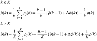
In principle, the more epochs of data that are used in the smoothing process, the more precise the smoothed pseudorange should become, and it should approach the precision of the carrier range. However, if the averaging constant is increased beyond a certain point, the filter diverges because the ionosphere delays the pseudorange and advances the carrier range. This effect is called the ionospheric divergence, and this effect increases with the averaging constant k. With a reduction in the ionospheric divergence, the variable k remains constant when it reaches K.

(1)

$\eqalign{\tab k\les K \cr \tab \hat{\rho }\lpar k\rpar \equals {1 \over k}\sum\limits_{j \equals \setnum{1}}^{k} {\rho _{j} } \lpar k\rpar \equals {{k \minus 1} \over k}\lcub \hat{\rho }\lpar k \minus 1\rpar \plus \rmDelta \phi \lpar k\rpar \rcub \plus {1 \over k}\rho \lpar k\rpar \cr \tab k \gt K \cr \tab \hat {\rho} \lpar k\rpar \equals {1 \over K}\sum\limits_{j \equals \setnum{1}}^{K} {\rho _{j} } \lpar k\rpar \equals {{K \minus 1} \over K}\lcub \hat{\rho }\lpar k \minus 1\rpar \plus \rmDelta \phi \lpar k\rpar \rcub \plus {1 \over K}\rho \lpar k\rpar \cr}$

where:

ρ(k): raw pseudorange measurement at the current epoch,
Δφ(k): change in carrier phase,
$\hat{\rho }\lpar k\rpar$: smoothed pseudorange at the current epoch,
$\hat{\rho }\lpar k \minus 1\rpar$: smoothed pseudorange at the previous epoch,
k: smoothing window width of Hatch filter,
K: maximum value of k.

At one observation per second, a maximum of 100 seems a good value for K, and the FAA reported it as the LAAS recommendation. It is, however, a recommended value not an optimal one. The value of K depends on where and when the GPS measurements are made, so we need to focus on reducing both the ionosphere-induced and measurement-noise error sources.

The estimated pseudorange (ρ_m(k)) for the current epoch (k) uses pseudorange (ρ_m(m)) and carrier phase (φ_m(m)) measurement of the past epoch (m) and includes the ionosphere-induced error $\minus 2\bar{i}_{dot} \cdot \lpar k \minus m\rpar$ and measurement noise.

(2)

$\eqalign{\rho _{m} \lpar k\rpar \tab \equals \rho _{m} \lpar m\rpar \plus \lcub \phi \lpar k\rpar \minus \phi \lpar m\rpar \rcub \cr \tab \equals \rho _{true} \lpar k\rpar \minus 2 \cdot \bar{i}_{dot} \cdot \lpar k \minus m\rpar \plus v_{\rho } \lpar m\rpar \plus v_{\phi } \lpar k\rpar \plus v_{m} \lpar m\rpar \cr \tab \equals \u{\rho } \lpar k\rpar \plus v_{\rho } \lpar m\rpar \plus v_{\phi } \lpar k\rpar \plus v_{m} \lpar m\rpar \cr}$

where:

$\bar{i}_{dot}$: average time-rate in ionospheric delay,
$\u{\rho}$: estimated pseudorange including ionosphere-induced error,
v _ρ: pseudorange measurement noise,
v _φ: carrier phase measurement noise.

After the first K epoch, the smoothing window width (k) should remain constant. Generally, the value K is far smaller than the total observable epochs of each satellite, so it is reasonable to concentrate on the second equation in (1), which is normally suitably applied.

If we gather together the estimations of the last K epochs to smooth the current measurement, the estimated pseudorange has the noise expressed in equation (3).

(3)

$\eqalign{\tab \rho _{k} \lpar k\rpar \equals \u{\rho } \lpar k\rpar \plus v_{\rho \lpar k\rpar } \cr \tab \rho _{k \minus \setnum{1}} \lpar k\rpar \equals \u{\rho } \lpar k\rpar \plus v_{\rho \lpar k \minus \setnum{1}\rpar } \plus v_{\phi \lpar k\rpar } \plus v_{\phi \lpar k \minus \setnum{1}\rpar } \cr \tab \rho _{k \minus \setnum{2}} \lpar k\rpar \equals \u{\rho } \lpar k\rpar \plus v_{\rho \lpar k \minus \setnum{2}\rpar } \plus v_{\phi \lpar k\rpar } \plus v_{\phi \lpar k \minus \setnum{1}\rpar } \cr \tab \hskip30pt\vdots\cr \tab \rho _{k \minus K \plus \setnum{1}} \lpar k\rpar \equals \u{\rho } \lpar k\rpar \plus v_{\rho \lpar k \minus K \plus \setnum{1}\rpar } \plus v_{\phi \lpar k\rpar } \plus v_{\phi \lpar k \minus K \plus \setnum{1}\rpar } \cr \tab \_\!\_\!\_\!\_\!\_\!\_\!\_\!\_\!\_\!\_\!\_\!\_\!\_\!\_\!\_\!\_\!\_\!\_\!\_\!\_\!\_\!\_\!\_\!\_\!\_\!\_\!\_\!\_\!\_\!\_\!\_\!\_\!\_\!\_\!\_\!\_\!\_\!\_\!\_\!\_\!\_\!\_\!\_\!\_\!\_\!\_\!\_\!\_\!\_\!\_\!\_\!\_\!\_\!\_\!\_\!\_\!\_\!\_\!\_\!\_\!\_\!\_\!\_\!\_\!\_\!\_\!\_\!\_\!\_\!\_\!\_\!\_\!\_\!\_\!\_\!\_\!\_\!\_\!\_\!\_\!\_\!\_\!\_\!\_\!\_\!\_\!\_\!\_\!\_\!\_\!\_\!\_\!\_averaging \cr \tab \hat{\rho }\lpar k\rpar \equals \u{\rho } \lpar k\rpar \plus {1 \over K}\lcub v_{\rho \lpar k\rpar } \plus v_{\rho \lpar k \minus \setnum{1}\rpar } \plus \cdots \plus v_{\rho \lpar k \minus K \plus \setnum{1}\rpar } \rcub \cr \tab \quad\quad\ \plus {1 \over K}\lcub \lpar K \minus 1\rpar v_{\phi \lpar k\rpar } \plus v_{\phi \lpar k \minus \setnum{1}\rpar } \plus v_{\phi \lpar k \minus \setnum{2}\rpar } \plus \cdots \plus v_{\phi \lpar k \minus K \plus \setnum{1}\rpar } \rcub \cr}$

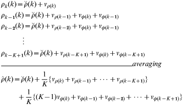
Recalling that the carrier noise is far smaller than that of the code and that these have similar properties to those of white noise, the estimation noise (N(k)) can be simplified as equations (4) and (5).

(4)

$\eqalign{ N\lpar k\rpar \equals \tab {1 \over K}\lcub v_{\rho \lpar k\rpar } \plus \cdots \plus v_{\rho \lpar k \minus K \plus \setnum{1}\rpar } \rcub \plus {1 \over K}\lcub \lpar K \minus 1\rpar v_{\phi \lpar k\rpar } \plus v_{\phi \lpar k \minus \setnum{1}\rpar } \plus \cdots \plus v_{\rho \lpar k \minus K \plus \setnum{1}\rpar } \rcub \cr \approx \tab {1 \over K}\lcub v_{\rho \lpar k\rpar } \plus \cdots \plus v_{\rho \lpar k \minus K \plus \setnum{1}\rpar } \rcub \cr}$

(5)

$\eqalign{ E\lpar N\lpar k\rpar ^{T} N\lpar k\rpar \rpar \equals \tab {{\lcub v_{\rho \lpar k\rpar } \plus \cdots \plus v_{\rho \lpar k \minus K \plus \setnum{1}\rpar } \rcub ^{T} \lcub v_{\rho \lpar k\rpar } \plus \cdots \plus v_{\rho \lpar k \minus K \plus \setnum{1}\rpar } \rcub } \over {K^{\setnum{2}} }} \cr \equals \tab {1 \over {K^{\setnum{2}} }}\lcub \sigma _{\rho \lpar k\rpar }^{\setnum{2}} \plus \sigma _{\rho \lpar k \minus \setnum{1}\rpar }^{\setnum{2}} \plus \cdots \plus \sigma _{\rho \lpar k \minus K \plus \setnum{1}\rpar }^{\setnum{2}} \rcub \approx {1 \over {K^{\setnum{2}} }}K\sigma _{\rho \lpar k\rpar }^{\setnum{2}} \equals {1 \over K}\sigma _{\rho \lpar k\rpar }^{\setnum{2}} \cr}$

The ionosphere delays the code and advances the phase, so it gives the estimation an ionosphere-induced error. Equation (6) shows that it reaches $\minus {{K \minus 1} \over K}2\bar{i}_{dot} \cdot 1$ for the last epoch, and the cumulative error for K epochs is expressed in Equation (7).

(6)

$\eqalign { \hat{\rho }\lpar k\rpar \tab \equals {{K \minus 1} \over K}\lcub \hat{\rho }\lpar k \minus 1\rpar \plus \rmDelta \phi \lpar k\rpar \rcub \plus {1 \over K}\rho \lpar k\rpar \cr \tab \equals {{K \minus 1} \over K}\lcub \hat{\rho }\lpar k \minus 1\rpar \plus \rmDelta \rho \lpar k\rpar \minus 2\bar{i}_{dot} \cdot 1\rcub \plus {1 \over K}\rho \lpar k\rpar \cr \tab \equals \rho _{true} \lpar k\rpar \minus {{K \minus 1} \over K}2\bar{i}_{dot} \cdot 1 \cr}$

(7)

$\eqalign{ \hat{\rho }\lpar k\rpar \tab \equals {{K \minus 1} \over K}\lcub \hat{\rho }\lpar k \minus 1\rpar \plus \rmDelta \rho \lpar k\rpar \minus 2 \cdot \bar{i}_{dot} \rcub \plus {1 \over K}\rho \lpar k\rpar \cr \tab \equals {{K \minus 1} \over K}\lcub \rho _{k \minus \setnum{1}} \lpar k\rpar \minus {{K \minus 1} \over K}2\bar{i}_{dot} \minus 2\bar{i}_{dot} \rcub \plus {1 \over K}\rho \lpar k\rpar \cr \tab \equals {{K \minus 1} \over K}\lcub \rho _{k \minus \setnum{2}} \lpar k\rpar \minus \left( {{{K \minus 1} \over K}} \right)^{\setnum{2}} 2\bar{i}_{dot} \minus \left( {{{K \minus 1} \over K}} \right)2\bar{i}_{dot} \minus 2\bar{i}_{dot} \rcub \plus {1 \over K}\rho \lpar k\rpar \cr}$

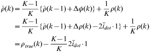
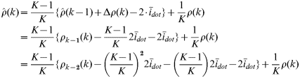
Assuming that the ionospheric delay varies linearly for K epochs, $\bar{i}_{dot} \equals {\rm constant}$ , the ionosphere-induced error (R(k)) is derived by Equation (8).

(8)

$\eqalign{ R\lpar k\rpar \tab \equals \minus \sum\limits_{i \equals \setnum{1}}^{K} {\left( {{{K \minus 1} \over K}} \right)^{i} } 2 \cdot \bar{i}_{dot} \equals \minus {{{{K \minus 1} \over K}\left\{ 1 \minus \left( {{{K \minus 1} \over K}} \right)^{K} \right\} } \over {1 \minus \left( {{{K \minus 1} \over K}} \right)}}2 \cdot \bar{i}_{dot} \cr \tab \equals \minus \lpar K \minus 1\rpar \left\{ 1 \minus \left( {1 \minus {1 \over K}} \right)^{K} \right\} \cdot 2 \cdot \bar{i}_{dot} \cr}$

(9)

$\mathop {\lim }\limits_{K \to \infty } \left( {1 \minus {1 \over K}} \right)^{ \minus K} \equals e$

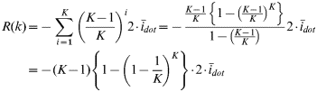
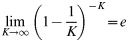
If K is great enough, the ionosphere-induced error (R(k)) can be simplified by Equation (10).

(10)

$R\lpar k\rpar \equals \minus \lpar K \minus 1\rpar \left\{ {1 \minus {1 \over e}} \right\} \cdot 2 \cdot \bar{i}_{dot}$

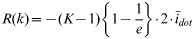
Therefore, the estimated pseudorange can be summarized as Equation (11), and we can find out the DRMS value of the pseudorange error in Equation (13).

(11)

$\hat{\rho }\lpar k\rpar \equals \rho _{true} \lpar k\rpar \plus N\lpar k\rpar \plus R\lpar k\rpar \equals \rho _{true} \lpar k\rpar \plus \delta \rho \lpar k\rpar$

(12)

$\eqalign{ DRMS^{\setnum{2}} \equals \tab E\hskip2\lsqb \delta \rho \lpar k\rpar ^{T} \delta \rho \lpar k\rpar \rsqb \cr \equals \tab E\hskip2\lsqb \lcub N\lpar k\rpar \plus R\lpar k\rpar \rcub ^{T} \lcub N\lpar k\rpar \plus R\lpar k\rpar \rcub \rsqb \cr \equals \tab E\hskip2\lsqb N\lpar k\rpar ^{T} N\lpar k\rpar \rsqb \plus R\lpar k\rpar ^{T} E\hskip2\lsqb N\lpar k\rpar \rsqb \plus E\hskip2\lsqb N\lpar k\rpar ^{T} \rsqb R\lpar k\rpar \plus R\lpar k\rpar ^{T} R\lpar k\rpar \cr}$

(13)

$\eqalign{ DRMS^{\setnum{2}} \equals \tab E\hskip2\lsqb N\lpar k\rpar ^{T} N\lpar k\rpar \rsqb \plus R\lpar k\rpar ^{T} R\lpar k\rpar \cr \equals \tab {1 \over K}\sigma _{\rho \lpar k\rpar }^{\setnum{2}} \plus \lpar K \minus 1\rpar ^{\setnum{2}} \left( {1 \minus {1 \over e}} \right)^{\setnum{2}} \cdot 4 \cdot \bar{i}_{dot}^{\,\,\setnum{2}} \quad \lpar \because E\hskip2\lsqb N\lpar k\rpar \rsqb \equals 0\rpar \cr}$

From Equation (13), we reconfirm that the pseudorange estimation has less noise but larger ionospheric error as the smoothing window width increases.

3. ALGORITHM

3.1. Optimal Averaging Constant

Equation (13) says that a large K makes the noise component in estimation error small but the ionospheric component large. It is a kind of trade-off problem, so an optimization is needed. For this, we take DRMS² to M (K). The optimal K minimizes the M (K), and it is in the root of Equation (14).

(14)

$\eqalign{\tab {d \over {dK}}M\lpar K\rpar \equals 2\lpar K \minus 1\rpar \left( {1 \minus {1 \over e}} \right)^{\setnum{2}} 4i_{dot}^{\setnum{2}} \minus {1 \over {K^{\setnum{2}} }}\sigma _{\rho }^{\setnum{2}} \cr \tab \equals 8\left( {1 \minus {1 \over e}} \right)^{\setnum{2}} \bar{i}_{dot}^{\,\,\setnum{2}} \cdot {1 \over {K^{\setnum{2}} }}\left\{ {K^{\setnum{3}} \minus K^{\setnum{2}} \minus {{\sigma _{\rho }^{\setnum{2}} } \over {8\left( {1 \minus {1 \over e}} \right)^{\setnum{2}} \bar{i}_{dot}^{\,\,\setnum{2}} }}} \right\} \equals 0 \cr}$

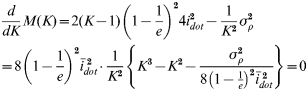
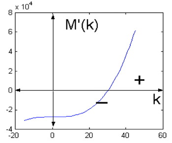
The smoothing constant K is a natural number, and the ${{\sigma _{\rho }^{\setnum{2}} } \over {8\left( {1 \minus {1 \over e}} \right)^{\setnum{2}} \bar{i}_{dot}^{\hskip2\setnum{2}} }}$ term in Equation (14) is a positive value, so the graph shape of ${d \over {dK}}M\lpar K\rpar$ is always similar to Figure 1. Accordingly, Equation (14) has only a root in the positive area, and M′ (K) changes from a negative to a positive value at this root, which means that the root makes the minimum value of M (K). Therefore, rounding the positive answer of Equation (14) to the nearest integer is the optimal smoothing window width of the Hatch filter.

Figure 1.

Graph shape of $<FT2>{d \over {dK}}M \lpar K \rpar$ .

3.2. Cardano's Method

One of the advantages of the Hatch filter is that it is a simple algorithm that is not a heavy load for the receiver process. When we apply the optimal constant to the classical Hatch filter, we should solve the cubic equation (15), and this can impose an additional heavy burden on the computing process.

(15)

$K^{\setnum{3}} \minus K^{\setnum{2}} \minus {{\sigma _{\rho }^{\setnum{2}} } \over {8\left( {1 \minus {1 \over e}} \right)^{\setnum{2}} \bar{i}_{dot}^{\hskip2\setnum{2}} }} \equals 0$

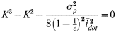
To keep the Hatch filter's merit as a simple algorithm, we bring Cardano's method to the calculation of the optimal averaging constant. This is a way of solving a class of cubic equations originally published in the 16th century by the Italian mathematician Gerolamo Cardano.

*************Cardano's Method*************

Cubic Equation: x ³+ax ²+bx+c=0

(16)

$\eqalign { x \equals \tab \root 3 \of {{1 \over 2}\left(\hskip-1pt {\minus q \plus \sqrt {q^{\setnum{2}} \plus 4p^{\setnum{3}} } } \right)} \plus \root 3 \of {{1 \over 2}\left( \hskip-1pt{\minus q \minus \sqrt {q^{\setnum{2}} \plus 4p^{\setnum{3}} } } \right)} \comma \cr \tab w\root 3 \of {{1 \over 2}\left( \hskip-1pt{\minus q \plus \sqrt {q^{\setnum{2}} \plus 4p^{\setnum{3}} } } \right)} \plus w^{\setnum{2}} \root 3 \of {{1 \over 2}\left( \hskip-1pt{\minus q \minus \sqrt {q^{\setnum{2}} \plus 4p^{\setnum{3}} } } \right)} \comma \cr \tab w^{\setnum{2}} \root 3 \of {{1 \over 2}\left( \hskip-1pt{\minus q \plus \sqrt {q^{\setnum{2}} \plus 4p^{\setnum{3}} } } \right)} \plus w\root 3 \of {{1 \over 2}\left( \hskip-1pt{\minus q \minus \sqrt {q^{\setnum{2}} \plus 4p^{\setnum{3}} } } \right)} \cr \tab where\comma {\rm \ }p \equals {1 \over 3}\left( \hskip-2pt{\minus {{a^{\setnum{2}} } \over 3} \plus b} \right)\comma \;q \equals {{2a^{\setnum{3}} } \over {27}} \minus {{ab} \over 3} \plus c\comma \;w^{\setnum{2}} \plus w \plus 1 \equals 0 \cr}$

***************************************

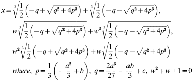
This method is still useful in Equation (15), and only the positive real root is available; therefore, the solution of Equation (15), K _temp, is expressed in Equation (17).

(17)

$\eqalign{\tab K_{temp} \equals \root 3 \of {{1 \over 2}\left( \hskip-1pt{\minus q \plus \sqrt {q^{\setnum{2}} \plus 4p^{\setnum{3}} } } \right)} \plus \root 3 \of {{1 \over 2}\left( \hskip-1pt{\minus q \minus \sqrt {q^{\setnum{2}} \plus 4p^{\setnum{3}} } } \right)} \plus {1 \over 3} \cr \tab where\comma \;p \equals {1 \over 3}\left( \hskip-2pt{\minus {1 \over 3}} \right)\comma \;q \equals \minus {2 \over {27}} \minus {{\sigma _{\rho }^{\setnum{2}} } \over {8\left( {1 \minus {1 \over e}} \right)^{\setnum{2}} \bar{i}_{dot}^{\hskip2pt\setnum{2}} }} \cr}$

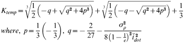
The optimal smoothing constant K _opt is an integer value, so we can get it by rounding K _temp to the nearest integer.

(18)

$K_{opt} \equals Roundoff\lpar K_{temp} \rpar$

3.3. Measurement Noise Statistics

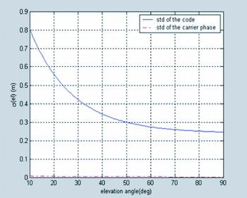
The measurement noise depends on the elevation angle, resulting primarily from the antenna gain pattern and signal attenuation due to atmospheric effects. Lower satellites are subject to substantially higher noise; however, different hardware might produce different noise, depending on the elevation angle (Grejner, Reference Grejner-Brzezinska and Toth2001).

In this paper, we used a Trimble 4000ssi Receiver Model for a simulation and DGPS test, so the receiver model that was introduced by Kee (Reference Kee1996) is useful for this algorithm. The standard deviation for each increment of elevation angle is fitted to Equation (19), and the parameters are summarized in Table 1. The standard deviation of pseudorange varies from 0·24 to 0·80 m as the elevation angle reduces from 90 deg to 10 deg, which is expressed in Figure 2.

(19)

$\sigma \lpar Ele\rpar \equals x_{\setnum{0}} \plus x_{\setnum{1}} \cdot e^{\left( \hskip-1{ \minus {{Ele} \over {x_{\setnum{2}} }}} \right)}$

Figure 2.

Noise statistics for L1 measurement.

Table 1.

Parameters for receiver noise.

3.4. Ionospheric Model

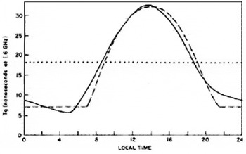
Receivers limited to L1 measurement have recourse to an empirical model whose parameter values are broadcast by the satellite. This is referred to as the Klobuchar model and represents the zenith delay as a constant value at night-time and a half-cosine function in the daytime as shown in Equation (20) and Figure 3. Eight parameters in the navigation message, local time and pierce point can be used to calculate the ionospheric vertical delay. The Klobuchar model represents the zenith delay as a constant value at nighttime and a half-cosine function in the daytime with a maximum at 2 pm local time. Update of the Klobuchar model coefficients occurs when there is a significant change in the 10·7 cm solar flux. This is combined with an obliquity factor dependent on the elevation angle.

(20)

$\eqalign{\tab \rmDelta t_{\setnum{1}} \equals A_{\setnum{1}} \plus A_{\setnum{2}} \cos \lsqb 2\pi \lpar t_{local} \minus A_{\setnum{3}} \rpar \sol A_{\setnum{4}} \rsqb {\rm \ } \cr \tab where \cr \tab A_{\setnum{1}} \equals 5 \times 10^{ \minus \setnum{9}} s \cr \tab A_{\setnum{2}} \equals \alpha _{\setnum{1}} \plus \alpha _{\setnum{2}} \varphi _{IP} \plus \alpha _{\setnum{3}} \varphi ^{\setnum{2}} _{\hskip3 IP} \plus \alpha _{\setnum{4}} \varphi ^{\setnum{3}} _{\hskip3 IP} \cr \tab A_{\setnum{3}} \equals 14\colon 00^{h} {\rm \ local\ time} \cr \tab A_{\setnum{4}} \equals \beta _{\setnum{1}} \plus \beta _{\setnum{2}} \varphi _{IP} \plus \beta _{\setnum{3}} \varphi ^{\setnum{2}} _{\hskip3 IP} \plus \beta _{\setnum{4}} \varphi ^{\setnum{2}} _{\hskip3 IP} \cr \tab \alpha _{i} \comma \beta _{i{\rm \ }} {\rm are\ 8\ ephemeris\ parameters} \cr \tab \rmDelta t_{\setnum{1}} \colon \ {\rm delay\ time\lpar s\rpar \comma \ }t_{local} \colon {\rm \ local\ time} \cr \tab \varphi _{IP} \colon \ {\rm spherical\ distance\ of\ pierce\ point\ } \cr \tab {\rm \ \from\ \ \ \ \ geomagnetic \ pole} \cr}$

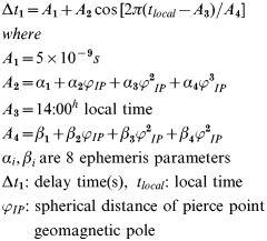
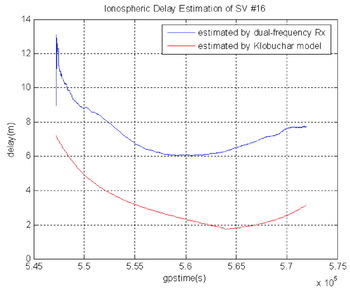
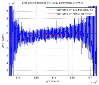
The dotted line in Figure 3 is obtained by this model, and the real value is shown as a solid line. Unfortunately, it is just a model and does not always describe the real world. It is generally accepted that it provides an estimate within 50% of the true delay. We can find this gap between the model estimation and the real delay in Figure 4. These data were obtained by the Youngju NDGPS reference station in Korea on a quiet day. The blue line is estimated using a dual-frequency receiver, and it is close to the real value, while the red line is calculated using the Klobuchar model with the ephemeris parameter of that day. The error is as high as 4 m, so there still remains an ionospheric error after using this model.

Figure 3.

Ionospheric delay estimation by the Klobuchar model.

Figure 4.

Ionospheric delay estimation by dual-frequency and Klobuchar model.

However, the model follows the tendency very well, as is shown in Figures 4 and 5. If we wish to estimate the current rate in quiet ionospheric delay, there is little problem in using this model.

Figure 5.

Ionospheric delay-rate estimation using dual-frequency receiver and Klobuchar model.

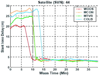
On the other hand, the tendency in ionospheric delay becomes very different on a stormy day. The tendency has already been studied by Ene et al. (Reference Ene, Qiu, Luo, Pullen and Enge2005). Figure 6 shows the tendency in a storm event. Because there is a steep gradient in the delay measurement in an ionospheric storm, the delay rate is much higher. Ene analysed the largest number of extreme ionosphere events of all the storms observed since Wide Area Augmentation System (WAAS) was fielded in the year 2000, and he concluded that ‘The other storms investigated, while potentially disruptive to civil aviation, fell well within the boundaries of the same threat model, as no events as critical as what was observed during the Autumn 2003 storms were found and confirmed’ (Ene, Reference Ene, Qiu, Luo, Pullen and Enge2005).

Figure 6.

Steep gradient measurement in a storm event [figure from Ene (Reference Ene, Qiu, Luo, Pullen and Enge2005) ].

Therefore, we set a conservative basic constant $\bar{i}_{dot}$ of the autumn 2003 storm as a worst case when a storm is noticed. A conservative high constant $\bar{i}_{dot}$ value weakens the noise performance but makes no critical bias. In conclusion, we use the Klobuchar model for a quiet day and the conservative constant $\bar{i}_{dot}$ value when a storm is noticed from the WAAS correction message.

3.5. Optimal Hatch filter constant

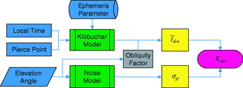
We have found that the optimal smoothing constant can be determined by a function of receiver noise and ionospheric variation in Equations (17) and (18). The measurement noise depends on the elevation angle in Equation (19), and the Klobuchar model is available to estimate the time rate in ionospheric delay on a quiet day. Now that we have the models, by inputting ephemeris parameter, local time, pierce point and elevation angle, we may get the measurement noise and time rate in ionospheric delay, which are definite components for the optimal constant. Therefore, we adopt a new function for elevation angle and ionospheric variation in the optimal Hatch filter constant.

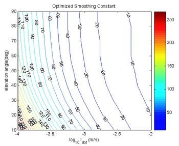
Using the suggested algorithm and noise model for the Trimble 4000ssi, we derive the optimal smoothing constant variation with the elevation angle and ionospheric delay rate as shown in Figure 7. In the case where the ionospheric delay varies slowly and the satellite is low lying, the optimal constant will be large. On the other hand, the limited measurement noise from a high elevation angle and a fast-moving ionosphere makes it small. When a storm is detected, a high basic constant $\bar{i}_{dot}$ value is used, and the optimal constant will be very low.

Figure 7.

Optimal smoothing constant variation.

To obtain a representative value, we took the mean elevation angle and time rate in ionospheric delay for all satellites during 24 hr on 24 May at Seoul, Korea as a quiet-day example. The mean values are summarized in Table 2, and inputting these to the function in Figure 8 gives the optimal constant 65. When we use the classical Hatch filter, we therefore expect that the smoothing window width of 65 will give the best DGPS performance.

Figure 8.

Block diagram for the optimal Hatch filter constant.

Table 2.

The mean value of the parameters for the optimal Hatch filter.

To see whether the suggested optimal averaging constant is effective for the classical Hatch filter, we did a 24 hr DGPS test for the various constants of 10, 30, 50, 70, 100, 200, and 300, and the results are summarized in Table 3. Using the same data as used in the previous analysis, we concluded that the constant that produced the best result was near 50. Considering that the averaging constant ranges from 0 to 1,000 or more and that the estimation was made by model, not by measurement, 50 is very close to the theoretical optimal constant of 65.

Table 3.

Classical Hatch filter DGPS result (2DRMS, m) with various smoothing constants.

4. ADAPTIVE WINDOW WIDTH ALGORITHM AND SIMULATION

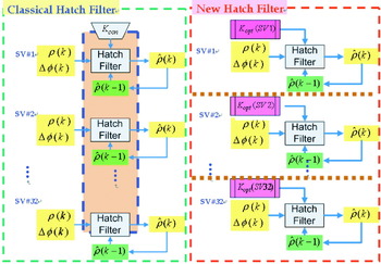
The classical Hatch filter uses a fixed smoothing constant for each satellite throughout the day as shown in the left block diagram in Figure 9. According to our new algorithm, this is not optimal. A number of satellites are rising, others are overhead, and some are setting. In the morning, the ionosphere changes quickly, but at night, it is quiescent. Should K remain constant for all satellites throughout? A small averaging constant should be applied to the measurement of the low-lying satellite in the morning, because then the ionospheric divergence may be enlarged by the Hatch filter with a large smoothing window. On the other hand, we feel that it is safe to broaden the window size for a high-elevation-angle satellite in the afternoon.

Figure 9.

Classical Hatch filter and new Hatch filter algorithm.

We suggest the flexible application of a different smoothing width $K_{SV_{i} } \lpar t\rpar$ for each satellite and each epoch. It is not a complex filter but a recursive one, which is added by one line of code in the existing receiver as shown in the right panel of Figure 9. We can therefore improve single-frequency receiver performance while maintaining the key advantage of the Hatch filter.

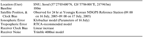
We did a simulation to verify that the new algorithm works well as summarized in Table 4. The reference station and user are located in Seoul. The 24 hr satellite positions and clock bias are calculated for the Youngju Korean NDGPS reference station in July. The ionospheric error varies based on the Klobuchar model whose ephemeris parameters are obtained by the station. The noise model is that of the Trimble 4000ssi receiver.

Table 4.

Adaptive smoothing window simulation summary.

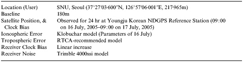
We derived the position from a stand-alone DGPS without filtering, a DGPS with Hatch filter whose averaging constant is 100, and an optimal Hatch filter with a adaptive smoothing width. For the performance comparison, we calculated the DGPS result for the divergence-free hatch filter using a dual-frequency receiver.

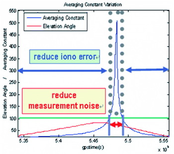
Figure 10 shows the variation of the optimal constant of PRN 14. It increases to 500, but for the classical Hatch filter remains at 100 throughout the day. For a low elevation angle, the optimal averaging constant is far smaller than 100, but it increases as the satellite moves overhead.

Figure 10.

Averaging constant variation with elevation angle.

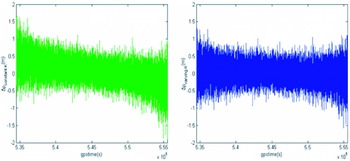
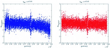
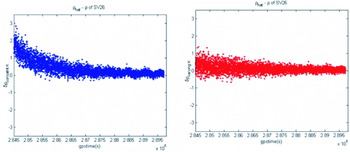
Figure 11 shows the comparison of PRN 14 pseudorange error between the classical Hatch filter and the new algorithm while the averaging constant varies as in Figure 10. The classical averaging constant, 100, is too large for low-elevation-angle measurement to have ionosphere-induced error in the shape of a bias. The new filtering algorithm keeps a small constant to reduce the ionospheric variation effect. On the other hand, the measurement noise for a high elevation angle is safely decreased by a large amount, because the ionospheric delay changes slowly.

Figure 11.

The classical (left) and optimal (right) Hatch filter error on the estimated pseudorange.

As noted before, the optimal constant depends on the elevation angle and ionospheric variation. Each elevation angle for the same epoch is different, so any two optimal constants are not the same in Table 5. Generally, we note that the higher the elevation angle, the larger the constant. The smoothing window widths are not equal in spite of the same elevation angle in Table 6 because the ionosphere varies not only in elevation angle but also in the pierce point and the measured time. Like these, the different constants are applied to different satellites, elevation angles, ionospheric variations and epochs by our new algorithm.

Table 5.

The optimal constants for the same epoch.

Table 6.

The optimal constants for the same elevation angle.

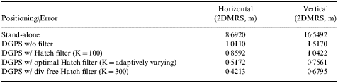
Figure 12 and Table 7 are the results of the simulation. Noise and occasionally severe bias are shown for the classical Hatch filter, but the optimal Hatch filter reduces both of these. The classical filter reduces the error by 15–30%, whereas our new algorithm decreases the error by 50%. From the result, the performance of our suggested filter algorithm using a single frequency matches that of a divergence-free Hatch filter that uses a dual-frequency signal.

Figure 12.

DGPS horizontal (left) and vertical (right) simulation results.

Table 7.

DGPS simulation results.

5. DGPS TEST AND RESULTS

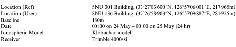
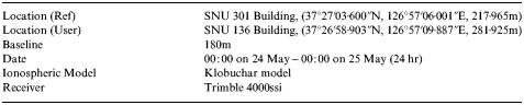
To check that our proposed algorithm with an improved performance is still effective for real data, we constructed a DGPS test system. It is explained in Table 8 and was made using the same data employed for the 24 hr optimal Hatch filter test. The Trimble 4000ssi was selected as the receiver type for the reference and user stations, and we used its noise statistics and the Klobuchar model for the optimal Hatch filter with a real-time adaptive smoothing window algorithm.

Table 8.

DGPS test construction.

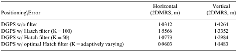
From our previous results, we concluded that the best performance from these data can be obtained when the smoothing width was fixed to 50. Therefore, we compared the DGPS results obtained by the new technique with those of 50 and 100.

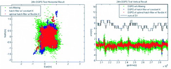
These results are shown in Table 9 and Figure 13. The traditional Hatch filter with 50 epoch smoothing did not improve the horizontal position accuracy and reduced the vertical error by 0·13 m (2DRMS) for 24 hr. The optimal Hatch filter with adaptive window width gave a better horizontal and vertical accuracy. The respective decrement seen is 0·07 m and 0·28 m (2DRMS). The errors for the fixed constant are smoothed but have some jumps as shown by the blue dots in Figure 13. The new algorithm brings these jumps to the true position as well as reducing the noise (red dots). The vertical error of DGPS with a constant K of 50 is as high as 4 m in the worst case, but it can be mitigated to under 3 m by our filtering algorithm.

Figure 13.

DGPS horizontal (left) and vertical (right) results.

Table 9.

DGPS test results.

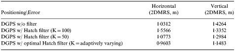
The new filter smoothes the errors as does the former one. Our smoothing performance is best, but the difference is not large. Examining the vertical results and the satellite constellation in the right graph in Figure 13, we see that the optimal Hatch filter is robust to the low satellites, while the classical Hatch filter is not. It can reduce the vertical error of the Hatch filter by 2 m.

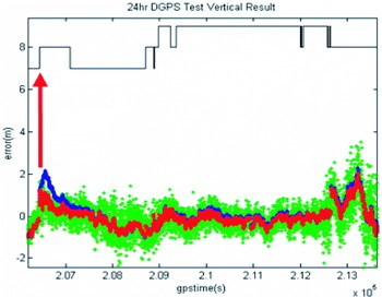
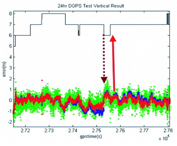
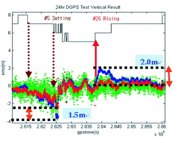
The following plots show how the low-elevation-angle satellite has affected the DGPS position accuracy with a classical Hatch filter. As soon as a new satellite rises as shown in Figure 14, the error jumps and returns to near zero after about 1000 sec. For about 1500 sec before the setting of a low-elevation-angle satellite in Figure 15, the positions are very noisy and biased. After a new satellite rises, the error increases as in Figure 14. The suggested Hatch filter causes the position to be robust to a low-elevation case, and it reduces the vertical position error of a traditional filter by as much as 2 m as seen in Figure 16.

Figure 14.

Low-elevation-angle positioning result (rising satellite case).

Figure 15.

Low-elevation-angle positioning result (rising and setting satellite case).

Figure 16.

Positioning accuracy improvement for low-elevation-angle satellite case.

If we look at what is happening to the averaging constant for rising and setting, the reason why the new algorithm is robust to a low-elevation-angle satellite is easily explained. We cannot forecast when this satellite will fall away, so the classical Hatch filter uses the fixed constant right before the satellite sets and causes a large ionosphere-induced error on the pseudorange estimation just before setting (left in Figure 17). However, the new algorithm can reduce it as shown in the right panel in Figure 17, because the low elevation gives much noise and reflects rapid ionosphere variation, and these narrow the smoothing window.

Figure 17.

Pseudorange error of a classical (left) and new (right) Hatch filter for a setting satellite (PRN #5).

A rising satellite case is similar to the previous one. For the first 50 epochs, the classical averaging constant increases continuously. It is still often large enough to inhibit an ionospheric divergence error as in the Figure 18 case. The optimal averaging constant slowly increases until the measurements may be safely smoothed.

Figure 18.

Pseudorange error of a classical (left) and new (right) Hatch filter for a rising satellite (PRN #26).

6. CONCLUSIONS

We can maximize the less expensive single-frequency receiver performance by adding the one line of Equation (17). This equation is useful in maximizing classical Hatch filter performance. Using 24 hr DGPS data, we verified that it derives the optimal constant reflected by the regional and receiver characteristics on a quiet day. We can also prevent a DGPS user experiencing severe bias due to a steep ionospheric delay gradient on a stormy day.

In applying our method to each epoch and satellite, we suggest a new optimal Hatch filter algorithm with an adaptive window width. The optimal Hatch filter we suggest maintains all the advantage of the classical Hatch filter. It is still recursive and simple and does not need any dynamic model or additional filter for time propagation. By using it, we can improve accuracy by 15%. Moreover, it is very robust to all the epochs, especially to those with low-lying satellites, and it occasionally reduces error jump by 2 m. The improvement of 15% (0·15 m) may not be so large because the 2DRMS value was calculated with the sense of 24 hr averaging. The user who obtains a position epoch by epoch will, however, see a 2 m error reduction as great progress.

If in future we have a smart ionospheric model that can estimate the tendency very well, our inexpensive single-frequency receiver will be able to compete with a highly priced dual-frequency receiver in DGPS positioning.

ACKNOWLEDGEMENT

The study was supported in part by in part by the Brain Korea 21 (BK-21) Program for Mechanical and Aerospace Engineering Research, the Institute of Advanced Machinery and Design, and Institute of Advanced Aerospace Technology at Seoul National University.

References

REFERENCES

Ene, A., Qiu, D., Luo, M., Pullen, S. and Enge, P. (2005). A Comprehensive Ionosphere Storm Data Analysis Method to Support LAAS Threat Model Development, the Institute of Navigation National Technical Meeting, San Diego CA, pp 110–130Google Scholar

Park, B. (2003). Comparison of the DGPS performance by various PRC filtering methods, MS thesis, Seoul National University, pp 16–36Google Scholar

Park, B. et al. (2006). RRC Unnecessary for DGPS Messages, IEEE Transactions on Aerospace and Electronic Systems, 42 (3), pp 1149–1160CrossRef Google Scholar

Parkinson, B. (1996). Global Positioning System: Theory and Applications II, Progress in Astronautics and Aeronautics, pp 81–114.Google Scholar

Klepczynski, B. (2003). Systematic Effects in GPS and WAAS Time Transfers, 34th Annual Precise Time and Time Interval (PTTI) Meeting, Reston, Virginia, pp. 405–412.Google Scholar

Kee, C., Park, B., Kim, J., Choi, S. (2004). PRC Generation in Time-Latency: Is RRC Still Required Even If S/A Has Been Turned Off?, ION 2004 NTM, pp 869–874.Google Scholar

Kee, C., Park, B., Kim, J., Cleveland, A., Parsons, M., Wolfe, D. (2007). A Guideline on Establishing DGPS Reference Station Requirements, The Journal of Navigation, 61 pp 99–114.CrossRef Google Scholar

Kee, C. (1996), Quality Control Algorithm on Wide-area Reference Station for WAAS, ION 52nd Annual Meeting, Cambridge, Massachusetts, pp 487–495.Google Scholar

Jwo, D. (2004), ARMA Neural Networks for Predicting DGPS Pseudorange Correction, The Journal of Navigation, 57 pp 275–286.CrossRef Google Scholar

Kim, D. (2000), The Multipath Divergence Problem in GPS Carrier-Smoothed Code Pseudorange, Proceedings of 47th Annual Conference of the Canadian Aeronautics and Space, Ottawa, Ont, pp 161–163.Google Scholar

Yun, D. and Kee, C. (1999), Single-frequency Differential GPS Accuracy Improvement via Local Area Ionospheric Time Delay Model Development, Telecommunications Review, 9 (1), pp 33–49.Google Scholar

Grejner-Brzezinska, D and Toth, C. (2001), Performance Study of High-End Dual Frequency GPS Receivers Tightly Integrated with a Strapdown INS, Proc. 3rd International Symposium on Mobile Mappig, Cairo, Egypt.Google Scholar

Loomis, P. (1989), Correction Algorithms for Differential GPS Reference Station, The Journal of Navigation, 36 pp 179–193.CrossRef Google Scholar

Misra, P., and Enge, P. (2001), Global Positioning System – Signals, Measurements, and Performance Ganga-Jamura Press, pp 123–171.Google Scholar

RTCA (1999), Minimum Operational Performance Standards for Global Positioning System/Wide Area Augmentation System Airborne Equipment RTCAGoogle Scholar

Wullschleger, V. (2000), FAA LAAS Specification: Requirements for Performance Type 1, European Institutes of Navigation GNSS 2000 Conference.Google Scholar