1 Introduction
Flow control is an attractive and promising technology as it aims to alter and improve inherent flow behaviour by externally applied forces. Reduction of drag, suppression of instabilities, extension of parameter envelopes and enhancement of mixing are just a few objectives that could be accomplished by flow-control strategies. Despite its potential for technological advances, the design of flow-control schemes still poses significant challenges, principally among them the modelling of the flow behaviour and the accurate description of the disturbance environment.
Model-based approaches, based on a prescribed set of equations and an a priori assumption on the characteristics of the noise environment, have been successfully applied to numerical simulations and have demonstrated their effectiveness within the range of design assumptions. For applications in experiments, in the absence of sufficient information on the disturbance environment, a different approach may be more appropriate which does not impose a preconceived model but rather extracts information for the control design, such as transfer functions, directly from measured (noise-contaminated) data. Techniques in this category rely on system-identification methods to obtain representations of the input–output behaviour of the flow; they fall into two major categories: subspace identification and Markov-parameter/realization techniques. Whereas the former exploits the low-rank nature of the control signal space to arrive at approximate system matrices via oblique projections (see, e.g., Katayama Reference Katayama2005), the latter first determines the discrete impulse responses (Markov parameters) of the flow, which are then, in a second step, used to derive a state-space model.
System identification has been an active field of research for many decades and has matured into a well-established discipline of system theory. Even though many techniques and algorithms are available, the use of system-identification techniques in the design of flow-control strategies is rather recent (see Huang & Kim Reference Huang and Kim2008; Hervé et al. Reference Hervé, Sipp, Schmid and Samuelides2012; Juillet, Schmid & Huerre Reference Juillet, Schmid and Huerre2013). For the identification of a reduced-order model that will form the basis of our control design, a two-step process is often advocated (see, e.g., Hjalmarsson Reference Hjalmarsson2005). It consists of a high-order identification of a preliminary model that best fits the available data, which is subsequently transformed into a low-order representation by model-reduction techniques. The approach ensures favourable statistical properties, since the asymptotic efficiency of the high-order system can be shown to be inherited by the low-order system; furthermore, the thus reduced low-order system is optimal within the constraints given by the high-order system.
Following this principle, we choose a Markov-parameter/realization technique in this study. In particular, we use an ARMarkov/LS technique to convert measured data sequences into discrete impulse responses (Markov parameters) by assuming an underlying autoregressive model that explicitly contains the Markov parameters; the parameters of the autoregressive model are determined by a least-squares (LS) matching to the measured data. The Markov parameters are then used in the eigensystem realization algorithm (ERA) to arrive at a state-space representation of the model, which in turn can be used to design a control law by standard techniques. The ARMarkov/LS procedure was originally proposed by Akers & Bernstein (Reference Akers and Bernstein1997), and many subsequent studies (see Van Pelt & Bernstein Reference Van Pelt and Bernstein1998; Kamrunnahar, Huang & Fisher Reference Kamrunnahar, Huang and Fisher2000; Fledderjohn et al. Reference Fledderjohn, Holzel, Palanthandalam-Madapusi, Fuentes and Bernstein2010) have confirmed it as a very efficient technique to obtain the Markov parameters of a system. The ERA state-space realization step was developed by Juang & Pappa (Reference Juang and Pappa1985), has been studied extensively (see Lew, Juang & Longman Reference Lew, Juang and Longman1993) and has recently been applied to flow-control problems in the form of an adjoint-free model-reduction procedure (see Ma, Ahuja & Rowley Reference Ma, Ahuja and Rowley2011).
One of the advantages and appeals of data-based control design using system-identification techniques is its applicability to realistic flow situations, where the only information about the system to be controlled consists of (low-dimensional) measurements. This advantage is, however, offset by the uncertainty these signals introduce into the design process, since the processed data will surely be contaminated by background and measurement noise and ultimately affect the control performance. In particular, for a practical control design, it is important to quantify the noise in the data and how it propagates through the procedural steps of the system identification and control design to ultimately influence the control performance and its internal stability margins. A sensitivity analysis of this type is the focus of this article. Due to our two-step approach, we can break apart the error in the identification step into a variance estimation of the identified model and a bias estimation of the reduced-order model. This distinction is valid as long as the model-reduction step is robust, i.e. shows a negligible sensitivity of the model parameters to noise in the underlying data.
Computation of estimates of the variance and bias error with respect to variations in the model parameters for an identification–realization algorithm has been the topic of previous articles in the identification/realization literature. For example, the model-order criteria of Akaike (Reference Akaike1974) and Rissanen (Reference Rissanen1983) apply penalization techniques to a repeatability estimate to arrive at an objective model order (see Ljung Reference Ljung1987). In the study of Longman et al. (Reference Longman, Lew, Tseng and Juang1991), the model parameters for the ERA step were chosen based on statistical information of the identified variables. Besides its obvious benefits for control and stability calculations, the quantification of the variance and bias of the identification–realization parameters can also be used as a model structure falsification criterion (see Hjalmarsson Reference Hjalmarsson2005).
We will concentrate on linear models as well as a representative system-identification algorithm. The first choice is motivated by the widespread use of control theories, model-reduction algorithms and system extraction techniques that rely on the linear evolution of small perturbations about a steady base or mean flow. Even though a great many fluid systems are more aptly described by nonlinear equations, linear techniques are often applied and indeed applicable when small manipulations about quasistationary states are concerned. For example, transition in boundary layers, initiated by a low-amplitude disturbance environment, as encountered on aerofoils under cruise conditions, can be successfully described (and controlled) by a linear model. As for the second choice, we have selected a system-identification algorithm that directly targets the Markov parameters (temporally discrete impulse responses) using a least-squares fitting technique for a rational model. This commonly applied algorithm will act as a placeholder for many other techniques based on
 $z$
-transformed frequency responses; the uncertainty analysis presented here can thus be applied to various other related techniques with only minor modifications.
This paper is concerned with the propagation of uncertainties and stochastic fluctuations in the processed data through a multistep procedure based on system identification, state-space realization and optimal control design. In particular, we wish to quantify how small perturbations in the data will ultimately affect closed-loop control performance and degrade internal stability margins. As system-identification techniques are increasingly applied to fluid dynamical systems in an attempt to extract models upon which control strategies are to be designed (see, e.g., Huang & Kim Reference Huang and Kim2008; Hervé et al. Reference Hervé, Sipp, Schmid and Samuelides2012; Juillet et al. Reference Juillet, Schmid and Huerre2013), it appears prudent to assess the sensitivity of the models and the control to stochastic variability in the underlying data. We start in § 2 by presenting the ARMarkov/LS/ERA identification–realization algorithm for a single-input–single-output (SISO) system. Section 3 will then concentrate on a perturbation technique to derive estimates of the error between the real and identified models; this section naturally divides into two parts: quantifying the ARMarkov/LS identification error and deriving an ERA error estimate. A validation of these error estimates is presented in § 4, where we consider the flow over an idealized aerofoil and demonstrate the utility of sensitivity measures in the analysis of closed-loop control problems based on system identification and realization. Conclusions are presented in § 5.
2 From data sequences to control performance
We start by developing the essential steps in the design of an efficient and robust control strategy, starting from input–output data sequences. These steps will consist of (i) a system-identification process, which matches the coefficients of a given model structure using observed input–output signals, (ii) a design of a feedback or feed-forward controller and (iii) the assessment of gain and phase margins of the compensated system.
2.1 General framework for linear time-invariant systems
We choose a discrete-time state-space representation to describe the flow-control set-up for a linear time-invariant (LTI) system and consider a single input and single output (i.e. a SISO system). The restriction to SISO systems does not pose limitations on the applicability of our analysis to more complex control settings, such as multiple-input–multiple-output (MIMO) systems. It has mostly been chosen for clarity of exposition and to focus on the conceptual uncertainty-propagation framework, rather than on full generality. In our SISO derivation below, our Markov parameters (discrete impulse responses) are scalars, while for the more involved MIMO case they constitute
 $n_{o}\times n_{i}$
matrices, with
 $n_{o}$
and
 $n_{i}$
as the numbers of output (sensor) and input (actuator) signals respectively; the essential steps in the analysis can readily be extended to the MIMO case. We have
 $$\begin{eqnarray}\displaystyle & \boldsymbol{x}(k+1)=\unicode[STIX]{x1D63C}\,\boldsymbol{x}(k)+\unicode[STIX]{x1D63D}u(k)+\boldsymbol{w}(k), & \displaystyle\end{eqnarray}$$
 $$\begin{eqnarray}\displaystyle & y(k)=\unicode[STIX]{x1D63E}\boldsymbol{x}(k)+Du(k)+g(k), & \displaystyle\end{eqnarray}$$
 $k$
denotes the discrete-time index,
 $\boldsymbol{x}(k)$
represents the state vector,
 $u(k)$
is the control,
 $y(k)$
stands for the measurement, and
 $\boldsymbol{w}(k)$
and
 $g(k)$
are the state noise and measurement uncertainties respectively. The system matrix is given by
 $\unicode[STIX]{x1D63C}$
, the actuation is modelled by
 $\unicode[STIX]{x1D63D}$
and the sensors by
 $\unicode[STIX]{x1D63E}$
. Finally,
 $D$
describes the instantaneous effect of the actuation on the measurement, also referred to as the throughput. For a system of order
 $n$
, the system matrix
 $\unicode[STIX]{x1D63C}$
is
 $n\times n$
, the actuation matrix
 $\unicode[STIX]{x1D63D}$
and the plant noise
 $\boldsymbol{w}$
are
 $n\times 1$
, the sensor matrix
 $\unicode[STIX]{x1D63E}$
is
 $1\times n$
, and
 $D$
and
 $g$
are scalar quantities.
The impulse response of the above system (2.1), in the case of vanishing noise terms, can be defined as a sequence of scalars. This sequence is also referred to as the Markov parameters
 $H_{j}$
. From the state-space representation (2.1) an explicit form of the Markov parameters can be derived according to
 $$\begin{eqnarray}\displaystyle & H_{0}=D, & \displaystyle\end{eqnarray}$$
 $$\begin{eqnarray}\displaystyle & H_{j}=\unicode[STIX]{x1D63E}\unicode[STIX]{x1D63C}^{j-1}\unicode[STIX]{x1D63D},\quad j\geqslant 1. & \displaystyle\end{eqnarray}$$
 $\boldsymbol{x}(k)$
. Rather, the output at
 $k$
can be determined solely as functions of past inputs and outputs. The definition (2.2) of the Markov parameters
 $H_{j}$
then allows us to formulate a regressive representation of general LTI systems as a discrete transfer function from the input
 $u$
to the output
 $y$
. We obtain
 $$\begin{eqnarray}y(k)=\mathop{\sum }_{j=0}^{\infty }H_{j}u(k-j).\end{eqnarray}$$
An approximation of this model, assuming that after a certain time the effects of the actuations are negligible, is the well-known finite-impulse response (FIR) model of order
 ${\it\mu}$
. We have
 $$\begin{eqnarray}y(k)=\mathop{\sum }_{j=0}^{{\it\mu}-1}H_{j}u(k-j).\end{eqnarray}$$
A more sophisticated representation is given by applying an autoregressive term to the signal
 $y$
, which yields the well-known ARX (autoregressive-exogenous-input) model
 $$\begin{eqnarray}y(k)=\mathop{\sum }_{j=1}^{n}-N_{j}y(k-j)+\mathop{\sum }_{j=0}^{n}M_{j}u(k-j),\end{eqnarray}$$
where
 $M_{j}$
and
 $N_{j}$
are coefficients to be determined. Akers & Bernstein (Reference Akers and Bernstein1997) showed that the Markov parameters can be extracted from the ARX representation via the following recursive algorithm. Using (2.5) and the definition of the measurement
 $y$
we obtain, after repeated substitution, the following autoregressive representation which explicitly isolates
 ${\it\mu}$
Markov parameters (referred to as
 ${\it\mu}$
-ARMarkov):
 $$\begin{eqnarray}y(k)=\mathop{\sum }_{j=1}^{n}-P_{j}y(k-{\it\mu}-j+1)+\mathop{\sum }_{j=1}^{{\it\mu}}H_{j-1}u(k-j+1)+\mathop{\sum }_{j=1}^{n}Q_{j}u(k-{\it\mu}-j+1).\end{eqnarray}$$
To proceed, the
 ${\it\mu}$
-ARMarkov model may be written as a linear relation between
 $y(k)$
, a vector
 ${\bf\phi}(k)$
and the model parameters, grouped into the vector
 $\boldsymbol{W}$
, according to
 $$\begin{eqnarray}y(k)={\bf\phi}(k)\boldsymbol{W},\end{eqnarray}$$
where
 ${\bf\phi}(k)$
and
 $\boldsymbol{W}$
are given as
 $$\begin{eqnarray}{\bf\phi}(k)=\left[y(k-{\it\mu}),\ldots ,y(k-{\it\mu}-n+1),u(k),\ldots ,u(k-{\it\mu}-n+1)\right]\end{eqnarray}$$
and
 $$\begin{eqnarray}\boldsymbol{W}^{\text{T}}=\left[-P_{1},\ldots ,-P_{n},H_{0},\ldots ,H_{{\it\mu}-1},Q_{1},\ldots ,Q_{n}\right]\!.\end{eqnarray}$$
Equation (2.7) is a compact form of the autoregressive representation of (2.6) where
 ${\bf\phi}(k)$
contains the input–output sequence just before the
 $k$
th time index and
 $\boldsymbol{W}$
contains the ARMarkov parameters. The transfer functions based on the
 $z$
-transform of the above models (FIR, autoregressive moving average (ARMA) and
 ${\it\mu}$
-ARMarkov) are given in appendix A for completeness. The following section presents the algorithm proposed by Akers & Bernstein (Reference Akers and Bernstein1997) to identify the
 ${\it\mu}$
-ARMarkov parameters (in
 $\boldsymbol{W}$
) from input–output data sequences. Once the Markov parameters are identified (as a part of the vector
 $\boldsymbol{W}$
), the system behaviour is predicted using the FIR model (2.4). The other coefficients (i.e.
 $P_{i}$
and
 $Q_{i}$
) – even though ultimately not used – are to account for noise in the dataset and thus yield more accurate Markov parameters (see Kamrunnahar et al.
Reference Kamrunnahar, Huang and Fisher2000; Hjalmarsson Reference Hjalmarsson2005).
2.2 From data to an identified system: ARMarkov/LS
This section shows how the coefficients of the ARMarkov model are obtained from data sequences via a least-squares minimization. Many alternative techniques exist to identify model coefficients, in particular, for the ARMarkov representation. While details are kept to a minimum in what follows, the interested reader is referred to Ljung (Reference Ljung1987) and Hjalmarsson (Reference Hjalmarsson2005) for more information about the mathematical and algorithmic principles underlying system identification.
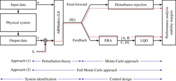
It will be emphasized here that the ARMarkov/LS algorithm is used to convert time sequences of the input and output signals into discrete impulse responses (Markov parameters), which in turn are fed to a realization algorithm (in our case, the ERA) to yield the system matrices of a state-space representation. A feedback controller can then be designed using standard techniques; a feed-forward controller can be devised directly from the identified transfer function. A sketch outlining the procedural steps is given in figure 1.
Outline of the procedural steps: from processed data, via system identification and control design, to performance analysis. The pathway in red indicates the uncertainty analysis, linking additive variance in the processed data to stability margins of the final control design. Approach (1), consisting of a perturbation part for the system identification, combined with a Monte Carlo approach for the control design, is pursued in this article; the alternative approach (2) is computationally far more costly, due to the high dimensionality of the input space.

2.2.1 The LS algorithm
Given an input–output dataset, a system-identification procedure is concerned with finding a model that can reproduce the output (
 $y$
) sequence using the input (
 $u$
) sequence. Formally,
 $y(k)$
is the array of measured outputs at time
 $k$
,
 $\boldsymbol{W}$
denotes a set of parameters that describe the model and
 $\widehat{y}(k\,\mid \,\boldsymbol{W})$
stands for the output computed using the input sequence and the model parameterized by
 $\boldsymbol{W}$
. The goal is to find
 $\boldsymbol{W}$
such that the sequence
 $\widehat{y}(k\,\mid \,\boldsymbol{W})$
best matches
 $y(k)$
. Thus, the ARMarkov/LS identification consists of minimizing
 $J$
given by
 $$\begin{eqnarray}J(\boldsymbol{W})=\frac{1}{N}\mathop{\sum }_{k=1}^{N}(y(k)-\widehat{y}(k\,\mid \,\boldsymbol{W}))^{2},\end{eqnarray}$$
with
 $N$
as the number of data points. For ARMarkov, the relationship between
 $\widehat{y}(k\,\mid \,\boldsymbol{W})$
and
 $\boldsymbol{W}$
is explicit and is given by (2.7). Substituting into (2.10) yields
 $$\begin{eqnarray}J(\boldsymbol{W})=\Vert \boldsymbol{Y}-{\it\Phi}\boldsymbol{W}\Vert _{2}^{2},\end{eqnarray}$$
with
 $$\begin{eqnarray}\boldsymbol{Y}=\left(\begin{array}{@{}c@{}}y({\it\mu}+n)\\ y({\it\mu}+n+1)\\ \vdots \\ y(N)\end{array}\right)\quad \text{and}\quad \unicode[STIX]{x1D731}=\left(\begin{array}{@{}c@{}}{\bf\phi}({\it\mu}+n)\\ {\bf\phi}({\it\mu}+n+1)\\ \vdots \\ {\bf\phi}(N)\end{array}\right).\end{eqnarray}$$
The minimization of
 $J(\boldsymbol{W})$
may be solved using the pseudoinverse to obtain
 $$\begin{eqnarray}\boldsymbol{W}={\it\Phi}_{{\it\epsilon}}^{\dagger }\boldsymbol{Y}.\end{eqnarray}$$
The coefficient vector
 $\boldsymbol{W}$
contains the Markov parameters
 $H_{j}$
. The pseudoinverse is often computed using Moore’s definition
 $$\begin{eqnarray}{\it\Phi}_{{\it\epsilon}}^{\dagger }\equiv ({\it\Phi}^{\text{T}}{\it\Phi}+{\it\epsilon}\unicode[STIX]{x1D644})^{-1}{\it\Phi}^{\text{T}},\end{eqnarray}$$
which minimizes a regularized cost functional
 $\widetilde{J}(\boldsymbol{W})$
of the form
 $$\begin{eqnarray}\widetilde{J}_{{\it\epsilon}}(\boldsymbol{W})=\Vert \boldsymbol{Y}-{\it\Phi}\boldsymbol{W}\Vert _{2}^{2}+{\it\epsilon}\Vert \boldsymbol{W}\Vert _{2}^{2}.\end{eqnarray}$$
The parameter
 ${\it\epsilon}$
can be set to machine precision, but it can also be used to enforce regularization of an otherwise ill-posed problem, as
 ${\it\Phi}$
is often rank-deficient. The term
 ${\it\Phi}$
contains the input–output data sequence: when the input does not consist of a broadband signal, the resulting LS problem becomes ill-posed. In this case, the use of Moore’s pseudoinverse definition allows us to implement a Tikhonov regularization of the problem (
 ${\it\epsilon}\neq 0$
, Fleming Reference Fleming2011). In this way, the norm of
 $\boldsymbol{W}$
remains bounded which, in turn, avoids numerical problems when using the identified model. In the different test cases presented in this paper, regularization is always applied with
 ${\it\epsilon}$
ranging from
 $10^{-5}$
to
 $10^{-16}$
(machine precision). The choice of
 ${\it\epsilon}$
depends on the application and the ill-posedness of the data sequence (
 ${\it\Phi}$
).
In order to have
 $\boldsymbol{W}$
represent the system dynamics rather than measurement noise, the minimization problem should be strongly underparameterized, i.e.
 $2n+{\it\mu}\ll N$
. In the limiting case of
 $2n+{\it\mu}=N$
, the input–output data sequence
 $(u,y)$
will be exactly matched by the reconstructed data
 $(u,\widehat{y})$
. In this case, the model parameters in
 $\boldsymbol{W}$
are strongly noise-dependent and are unlikely to be consistent with another set of data. In our examples, the parameters are chosen such that
 $2n+{\it\mu}<N/5;$
this choice is related to the AIC criterion defined below (see (2.16)). Even so, the model parameters in
 $\boldsymbol{W}$
are still dependent on noise, where the majority of this dependence is contained in the autoregressive part of
 $\boldsymbol{W}$
. For this reason, only the Markov parameters are kept (see Kamrunnahar et al.
Reference Kamrunnahar, Huang and Fisher2000; Hjalmarsson Reference Hjalmarsson2005), to minimize the noise dependence. The ARMarkov/LS procedure identifies all coefficients of the ARMarkov representation, but only an FIR (i.e. the set of Markov parameters) transfer function is kept. Still, with all of these precautions to identify a model that faithfully represents the system dynamics, the Markov parameters are influenced by noise, especially for a realistic dataset where the noise-to-signal ratio may be rather high. The uncertainty-propagation analysis aims to quantitatively estimate this dependence in order to improve the prediction of a controller’s performance.
2.2.2 Choice of data sequence
As we saw, the choice of the spectral content of the inputs has a significant impact on the statistical properties of the identified model, as it is related to the well-posedness of the minimization problem. The input signal has to be rich in frequencies that show a significant dynamic relevance in the physical system. In the absence of guiding information, a broad sweep through frequencies is commonly applied. However, since system-identification techniques are particularly attractive to experimental settings, the realizability of user-specified input signals becomes an additional point of concern. An attractive compromise consists of a pseudorandom binary signal (PRBS), a signal randomly changing between a zero and a unit state, which combines the requirements of a broadband frequency range, a simple relation between the duty cycle and the signal variance and, finally, a rather easy implementation in experiments by standard actuators. In numerical experiments with various input signals (e.g. chirp signals, random frequency sweeps etc.), the processing of data driven by a PRBS has yielded accurate and robust results. For further details on the choice and implications of the input signals, the reader is referred to the studies of Mehra (Reference Mehra1974), Brighenti, Wahlberg & Rojas (Reference Brighenti, Wahlberg and Rojas2009) and Gerencser, Hjalmarsson & Martensson (Reference Gerencser, Hjalmarsson and Martensson2009).
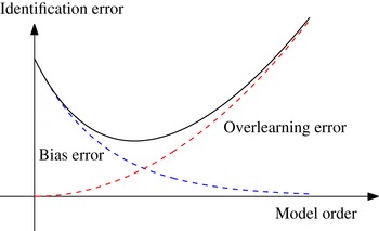
Sketch of the overlearning and bias error contributions to the total estimation error, as a function of the model order.

2.2.3 Model order and its link to model estimation error
The order of the model constitutes a crucial choice that has to be made in the identification process. For an ARMarkov model the order is
 $2n+{\it\mu}$
, while for an FIR model the order is simply
 ${\it\mu}$
. As shown previously, the model order is constrained, on one hand, by the length of the data sequence
 $2n+{\it\mu}\ll N$
. On the other hand, we have that
 $2n+{\it\mu}$
(and in particular
 ${\it\mu}$
since only an FIR is kept from the identification) has to be large with respect to the order of the model that describes the dynamics between the input and the output. A model order has to be chosen to balance these two criteria. Figure 2 graphically illustrates this balance that has to be struck. The bias error is related to an undermodelling of the dynamics, while the variance error is caused by a data sequence that is too small compared with the model order. An adequate model order can be found by various means. The very common Akaike criterion is chosen for our work (see Akaike Reference Akaike1974), which can be stated as
 $$\begin{eqnarray}\text{AIC}=\log (J(\boldsymbol{W}))+\frac{2}{N}\text{card}(\boldsymbol{W}).\end{eqnarray}$$
This value can be computed a posteriori, once a model has been determined. For model orders higher than Akaike’s criterion, see (2.16), the model error is assumed to be mostly due to variance error; for model orders below Akaike’s value, the model error is mostly due to bias error. The optimal model according to Akaike has a minimal AIC value. The criterion contains two terms. The first term
 $\log (J(\boldsymbol{W}))$
characterizes the residual minimization error, which is meant to represent the bias error of the identified model. Indeed, if the model order is sufficiently high, the problem becomes overparameterized and
 $J(\boldsymbol{W})$
consequently tends to zero. However, if the model order is rather low, the problem is overconstrained and
 $J(\boldsymbol{W})$
may not vanish. The second term in (2.16) denotes an index that is correlated with the variance error. It increases linearly with the number of parameters in the model and penalizes overparameterization. For our ARMarkov model, the cardinality
 $\text{card}(\boldsymbol{W})$
is the number of parameters
 $2n+{\it\mu}$
. The model order that minimizes AIC is taken as the optimal order for the identification procedure.
The uncertainty propagation developed later allows us to estimate the variance error; the bias error, however, is far harder to estimate, particularly when the noise-to-signal ratio is high. In order to take advantage of the variance error estimation, it is essential to choose a model order that is sufficiently high. What constitutes a sufficiently high order is difficult to define theoretically based on only the data sequence. For the remainder of the article, we base the model order on the minimal value of AIC given in (2.16).
2.3 From identified system to controller design
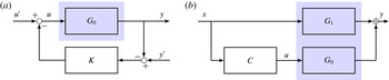
Once a model of appropriate order has been identified, a control strategy can be defined. Among the various choices to manipulate the flow, we will concentrate on two of the most common approaches: simple feedback control and simple feed-forward control. Both strategies are outlined in figure 3 in the form of a block diagram; they cover the most widely studied structures to control oscillatory and convectively dominated fluid flows.
Feedback (a) and feed-forward (b) control layout. The
 $G_{i}$
stand for transfer functions inherent to the system;
 $K$
and
 $C$
are the transfer functions of the respective controllers. The respective physical systems are indicated in shaded boxes.

In these configurations,
 $y$
represents the signal from the objective sensor which enters a user-specified objective function, and
 $u$
is the control variable, i.e. the signal passed to the actuator. In the feed-forward configuration, an additional sensor is present, which provides information about incoming disturbances and acts as a proxy for the (upstream) disturbance environment. In either configuration,
 $G_{i}$
stands for a transfer function describing the fluid behaviour between input and output signals; the transfer functions of the respective controllers are denoted by
 $K$
and
 $C$
respectively. For the feedback set-up, we also account for environmental noise sources, indicated by
 $u^{\prime }$
and
 $y^{\prime }$
. Before describing performance and stability criteria, we briefly outline common design algorithms for the two control configurations.
2.3.1 Feedback controllers
One of the most commonly applied strategies for feedback control is the infinite-time-horizon LQG/LQR control. After the identified system has been converted to a state-space representation, for example by using the ERA (Juang & Pappa Reference Juang and Pappa1985), a Kalman filter (for the optimal state estimation from measurements) and a proportional controller (which minimizes the control objective) can be designed. A large body of literature gives details of this design process; a data-based feedback approach applied to a fluid system can be found, e.g., in Illingworth, Morgans & Rowley (Reference Illingworth, Morgans and Rowley2011).
Regardless of the details of the designed controller, transfer functions of the feedback-controlled system can be expressed explicitly. They will be referred to as closed-loop transfer functions (CLTFs) throughout this paper. The CLTF describing the influence of the noise signal
 $u^{\prime }$
on the output
 $y$
reads
 $$\begin{eqnarray}T_{CL}=\frac{G_{0}}{1+G_{0}K},\end{eqnarray}$$
while the CLTF linking the noise signal
 $y^{\prime }$
to the same output is given by
 $$\begin{eqnarray}T_{CL}^{\prime }=\frac{G_{0}K}{1+G_{0}K}.\end{eqnarray}$$
2.3.2 Feed-forward controllers
This type of control is commonly applied to flows with a strongly convective behaviour, where disturbances originating upstream are to be compensated. In this set-up, an upstream sensor detects the incoming disturbances, after which an actuator counteracts them to create a nearly disturbance-free environment farther downstream (at the location of the objective sensor). General algorithms to design such controllers fall within the category of model predictive controllers (MPCs). Following the diagram in figure 3(b), the mapping between the measured incoming perturbations
 $s$
and the output (objective) sensor
 $y$
is given by the transfer function
 $G_{1}$
. An equivalent link between the actuator signal
 $u$
and the same output sensor
 $y$
can be established and described by the transfer function
 $G_{0}$
. The goal of the control design is then to construct a controller transfer function
 $C$
such that the signal passing through
 $C$
and
 $G_{0}$
destructively interferes with the signal passing though
 $G_{1}$
. It is straightforward to show that
 $C=-G_{0}^{-1}G_{1}$
provides a control law that accomplishes this task. Special care has to be exercised when inverting the transfer function
 $G_{0}$
, as substantially damped or eliminated frequencies in
 $G_{0}$
will yield numerical difficulties (or failure) during the inversion. For this reason, the inversion has to be understood as a regularized inversion, which can be accomplished, e.g., by Tikhonov regularization or by singular-value thresholding during pseudoinversion. As before, the transfer function of a system controlled by a feed-forward controller (from the upstream to the downstream sensor) can be stated explicitly. We will refer to it as the controlled-system transfer function (CSTF), given by
 $$\begin{eqnarray}T_{CS}=G_{1}+G_{0}C.\end{eqnarray}$$
2.4 From controller design to performance and stability: Nyquist and Bode plot analysis
The two transfer functions can be used to determine performance and stability measures. However, one has to keep in mind that the true transfer functions are not known; only their identified variants are available. To formally differentiate the exact and identified transfer functions, we introduce
 $G_{i}$
for the exact (but experimentally inaccessible) transfer function and
 $\widehat{G}_{i}$
for the nominal (identified) transfer function. Differences between these two transfer functions can be traced back to uncertainties or noise in the processed data.
For performance and stability studies, a simple substitution of
 $G_{i}$
by
 $\widehat{G}_{i}$
in (2.17) and (2.19) and a small-difference expansion can be applied for a first estimate of the influences of data corruption. In some high noise-to-signal cases, however, a different approach, involving a better approximation of the identification error, is called for. In the following section, we give a brief summary of stability criteria for the feedback (the Nyquist criterion) and feed-forward controller. Only stability issues will be dealt with in this article; uncertainty propagation, as introduced here, is not, however, limited to this output criterion.
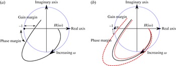
Nyquist plot of the OLTF, showing phase and gain margins, based on the nominal system (a) and the nominal system with uncertainty bounds (b).

2.4.1 The Nyquist stability criterion for feedback controllers
Considering the expressions in (2.17) and (2.18), the two CLTFs are singular when
 $G_{0}K=-1$
. This singularity is linked to the instability of the controlled system. The Nyquist plot is a representation of the open-loop transfer function (OLTF)
 $G_{0}K$
as a parameterized curve (by frequency) in the complex plane. The phase and gain margins defined by the Nyquist plot are measures that quantify the distance of the OLTF
 $G_{0}K$
from the point
 $-1$
in the complex plane. The phase margin is the maximally admissible phase variation of the system before stability is lost; the gain margin is the maximally admissible gain variation for the system to lose stability. The Nyquist curve can be recovered from the discrete-time transfer function (a function of
 $z$
) by a transformation to a continuous-time transfer function (a function of the frequency
 ${\it\omega}$
) via
 $z=\text{e}^{\text{i}{\it\omega}T_{e}}$
, where
 $T_{e}$
stands for the sampling time step of the data sequence.
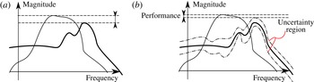
Figure 4 shows an example of a Nyquist plot. This figure gives a graphical definition of the phase and gain margins, as well as a potential reduction in the margins due to general uncertainties. For small noise-to-signal ratio the phase and gain margins can be satisfactorily estimated from the nominal system. As soon as uncertainties become more prevalent, the stability margins computed from the nominal system increasingly differ from the exact margins. In this latter case, uncertainty has to be directly taken into account to properly correct the margins.
2.4.2 Performance analysis for feed-forward disturbance rejection controllers
For feed-forward control configurations and strictly convective systems (i.e. with no feedback from the downstream input
 $u$
to the upstream sensor
 $s$
), the controller cannot be unstable. (In the presence of feedback from the downstream input
 $u$
to the upstream sensor
 $s$
, instabilities in the feed-forward control loop are possible; in this case, a state-space formulation would be more appropriate.) In this case, performance is of principal concern and constitutes the criterion for our analysis of uncertainty propagation. Performance will be defined using the maximum value of the CSTF (i.e. its
 $H_{\infty }$
norm). A controller is deemed effective if the maximum value of the transfer function without control is larger than the maximum value of the CSTF. Figure 5 provides a sketch of this criterion. In this figure, the uncontrolled and the controlled transfer function of the system are plotted, and the performance measure of the controller is evaluated. Similarly to the feedback configuration, uncertainty bounds about the nominal transfer function may yield a pronounced reduction of this nominal performance.
Bode diagram of the uncontrolled (thin black) and controlled (thick black) transfer functions, showing the
 $H_{\infty }$
-based performance of the nominal system (a) and the nominal system with uncertainty bounds (b).

3 Uncertainty propagation for the ARMarkov/LS identification process
We proceed by developing procedures to estimate uncertainty bounds in the identified system stemming from uncertainty in the processed data. In our case, we assume that the standard deviation of the data is known. First, the uncertainty propagation is demonstrated for the ARMarkov/LS identification algorithm, where the impact on the model parameters (Markov parameters and autoregressive parameters) is quantified. This is followed by establishing a link between the uncertainty in the Markov parameter and the resulting uncertainty bounds in the Bode and Nyquist diagrams. As a validation of this established procedure, a Monte Carlo variance estimation is then used, on a simple test case, to corroborate the uncertainty-propagation results by alternative means; since this validation step is advisable, but incidental to our development of a step-by-step procedure, we relegate this study to appendix B.
3.1 Variance error: linear perturbation analysis of the LS algorithm
Contrary to Monte Carlo techniques, we seek an explicit expression linking statistical information (such as the standard deviation) on the input data to an equivalent statistical measure of the Markov parameters. The uncertainty in the data is assumed to be additive; multiplicative uncertainty-propagation analyses can be found in Skogestad & Postlethwaite (Reference Skogestad and Postlethwaite2001), but will not be considered here. In addition, we restrict ourselves to sufficiently small measurement uncertainty in order to justify a first-order perturbation approach; furthermore, for simplicity, we assume noise-free input signals. The original data sequence, described by the vector
 $\boldsymbol{Y}$
, is perturbed as follows:
 $$\begin{eqnarray}\widetilde{\boldsymbol{Y}}=\boldsymbol{Y}+{\it\delta}\boldsymbol{Y}.\end{eqnarray}$$
The perturbations
 ${\it\delta}\boldsymbol{Y}$
are primarily perturbations of the input variables for the subsequent system-identification method. However, they have been generated by driving the physical system with a given input signal (in our case, PRBS) and hence contain, as subcomponents, measurement noise and observable plant noise. While a distinction between these two subcomponents will not be made, we acknowledge them as possible sources for the composite perturbation
 ${\it\delta}\boldsymbol{Y}$
. The influence of the perturbation
 ${\it\delta}\boldsymbol{Y}$
on the identified parameters (contained in
 $\boldsymbol{W}$
) can be quantified using (2.13). We note that, since
 $\unicode[STIX]{x1D731}$
contains past measurements, the size
 $N$
of the total data sequence differs from the number of equations
 $N-{\it\mu}-n+1$
. For this reason, two notations must be put forth: the vector of output data
 $\boldsymbol{Y}$
of size
 $N$
, and the solution
 $\boldsymbol{Y}_{t}$
of the LS problem of size
 $N-{\it\mu}-n+1$
:
 $$\begin{eqnarray}\left(\boldsymbol{W}+{\it\delta}\boldsymbol{W}\right)=\left(\unicode[STIX]{x1D731}+{\it\delta}\unicode[STIX]{x1D731}\right)_{{\it\epsilon}}^{\dagger }\left(\boldsymbol{Y}_{t}+{\it\delta}\boldsymbol{Y}_{t}\right).\end{eqnarray}$$
The resulting perturbation
 ${\it\delta}\boldsymbol{W}$
of the model parameters
 $\boldsymbol{W}$
is sought as a function of the perturbation
 ${\it\delta}\boldsymbol{Y}$
in the data
 $\boldsymbol{Y}$
. Under the previously mentioned assumption of small perturbations
 ${\it\delta}\boldsymbol{Y}$
, we linearize the above expression and derive a first-order perturbation solution for
 ${\it\delta}\boldsymbol{W}$
. This step is equivalent to linearizing the pseudoinverse term
 $\widetilde{\unicode[STIX]{x1D731}}_{{\it\epsilon}}^{\dagger }=\left(\unicode[STIX]{x1D731}+{\it\delta}\unicode[STIX]{x1D731}\right)_{{\it\epsilon}}^{\dagger }$
, a complex problem that has been the object of many past studies (see Wedin Reference Wedin1973; Stewart Reference Stewart1977, Reference Stewart1990). Following these studies, we can give an explicit expression for the model parameter perturbation
 ${\it\delta}\boldsymbol{W}$
(see Stewart Reference Stewart1977):
 $$\begin{eqnarray}{\it\delta}\boldsymbol{W}\approx \unicode[STIX]{x1D731}_{{\it\epsilon}}^{\dagger }{\it\delta}\boldsymbol{Y}_{t}+\left(-\unicode[STIX]{x1D731}_{{\it\epsilon}}^{\dagger }\unicode[STIX]{x1D64B}_{\unicode[STIX]{x1D731}}{\it\delta}\unicode[STIX]{x1D731}\unicode[STIX]{x1D64D}_{\unicode[STIX]{x1D731}}\unicode[STIX]{x1D731}_{{\it\epsilon}}^{\dagger }+(\unicode[STIX]{x1D731}^{\text{T}}\unicode[STIX]{x1D731})_{{\it\epsilon}}^{\dagger }\unicode[STIX]{x1D64D}_{\unicode[STIX]{x1D731}}{\it\delta}\unicode[STIX]{x1D731}^{\text{T}}\unicode[STIX]{x1D64B}_{\unicode[STIX]{x1D731}}^{\bot }-\unicode[STIX]{x1D64D}_{\unicode[STIX]{x1D731}}^{\bot }{\it\delta}\unicode[STIX]{x1D731}^{\text{T}}\unicode[STIX]{x1D64B}_{\unicode[STIX]{x1D731}}(\unicode[STIX]{x1D731}\unicode[STIX]{x1D731}^{\text{T}})_{{\it\epsilon}}^{\dagger }\right)\boldsymbol{Y}_{t},\end{eqnarray}$$
where
 $$\begin{eqnarray}\displaystyle \unicode[STIX]{x1D64B}_{\unicode[STIX]{x1D731}}\equiv \unicode[STIX]{x1D731}\unicode[STIX]{x1D731}_{{\it\epsilon}}^{\dagger },\quad \unicode[STIX]{x1D64D}_{\unicode[STIX]{x1D731}}\equiv \unicode[STIX]{x1D731}_{{\it\epsilon}}^{\dagger }\unicode[STIX]{x1D731}, & & \displaystyle\end{eqnarray}$$
 $$\begin{eqnarray}\displaystyle \unicode[STIX]{x1D64B}_{\unicode[STIX]{x1D731}}^{\bot }\equiv \unicode[STIX]{x1D644}-\unicode[STIX]{x1D64B}_{\unicode[STIX]{x1D731}},\quad \unicode[STIX]{x1D64D}_{\unicode[STIX]{x1D731}}^{\bot }\equiv \unicode[STIX]{x1D644}-\unicode[STIX]{x1D64D}_{\unicode[STIX]{x1D731}}. & & \displaystyle\end{eqnarray}$$
The matrix
 ${\it\delta}\unicode[STIX]{x1D731}$
contains perturbations of the data sequence. By definition, it can be directly expressed in terms of
 ${\it\delta}y(k)$
for
 $k\in [1,~N]$
according to
 $$\begin{eqnarray}{\it\delta}\unicode[STIX]{x1D731}=\left(\begin{array}{@{}ccccccc@{}}{\it\delta}y(n) & {\it\delta}y(n-1) & \ldots \, & {\it\delta}y(1) & 0 & \ldots \, & 0\\ {\it\delta}y(n+1) & {\it\delta}y(n) & \ldots \, & {\it\delta}y(2) & 0 & \ldots \, & 0\\ \vdots & \vdots & & \vdots & \vdots & \ddots & \vdots \\ {\it\delta}y(N) & {\it\delta}y(N-1) & \ldots \, & {\it\delta}y(N-n+1) & 0 & \ldots \, & 0\end{array}\right)\end{eqnarray}$$
or, in a more compact form,
 $$\begin{eqnarray}{\it\delta}\unicode[STIX]{x1D731}=\mathop{\sum }_{k=1}^{N}\unicode[STIX]{x1D640}(k){\it\delta}y(k),\end{eqnarray}$$
where we have introduced the operator
 $\unicode[STIX]{x1D60C}(k)_{i,j}$
as
 $$\begin{eqnarray}\unicode[STIX]{x1D60C}(k)_{i,j}=\left\{\begin{array}{@{}ll@{}}1 & \text{if }i-j+n=k\text{ and }i<n,\\ 0 & \text{elsewhere.}\end{array}\right.\end{eqnarray}$$
With this definition, we can reformulate the above relation between the data perturbations and the model parameter perturbations and state it in the form
 $$\begin{eqnarray}\displaystyle {\it\delta}\boldsymbol{W} & {\approx} & \displaystyle \unicode[STIX]{x1D731}_{{\it\epsilon}}^{\dagger }{\it\delta}\boldsymbol{Y}_{t}+\mathop{\sum }_{k=1}^{N}\left(-\unicode[STIX]{x1D731}_{{\it\epsilon}}^{\dagger }\unicode[STIX]{x1D64B}_{\unicode[STIX]{x1D731}}\unicode[STIX]{x1D640}(k)\unicode[STIX]{x1D64D}_{\unicode[STIX]{x1D731}}\unicode[STIX]{x1D731}_{{\it\epsilon}}^{\dagger }+(\unicode[STIX]{x1D731}^{\text{T}}\unicode[STIX]{x1D731})_{{\it\epsilon}}^{\dagger }\unicode[STIX]{x1D64D}_{\unicode[STIX]{x1D731}}\unicode[STIX]{x1D640}(k)^{\text{T}}\unicode[STIX]{x1D64B}_{\unicode[STIX]{x1D731}}^{\bot }-\unicode[STIX]{x1D64D}_{\unicode[STIX]{x1D731}}^{\bot }\unicode[STIX]{x1D640}(k)^{\text{T}}\unicode[STIX]{x1D64B}_{\unicode[STIX]{x1D731}}(\unicode[STIX]{x1D731}\unicode[STIX]{x1D731}^{\text{T}})_{{\it\epsilon}}^{\dagger }\right)\nonumber\\ \displaystyle & & \displaystyle \times \,\boldsymbol{Y}_{t}{\it\delta}y(k).\end{eqnarray}$$
Finally, this expression is equivalent to
 $$\begin{eqnarray}{\it\delta}\boldsymbol{W}=\unicode[STIX]{x1D647}{\it\delta}\boldsymbol{Y},\end{eqnarray}$$
where
 $\unicode[STIX]{x1D647}$
can be interpreted as the Jacobian of
 $\boldsymbol{W}$
with respect to
 $\boldsymbol{Y}$
. Consequently, the gradient of each component of
 $\boldsymbol{W}$
with respect to a specific perturbation in the processed data can be extracted from
 $\unicode[STIX]{x1D647}$
. We recall that only the Markov parameters
 $H_{i}$
are relevant for the representation of the system-identified model. With the definition of
 $\boldsymbol{W}$
, the propagation of data uncertainties into each Markov parameter can be found from (3.9). If we introduce the notation
 $\unicode[STIX]{x1D647}_{i}$
as the
 $i$
th row of the Jacobian
 $\unicode[STIX]{x1D647}$
, we obtain
 $$\begin{eqnarray}{\it\delta}H_{i}=\unicode[STIX]{x1D647}_{i+n}{\it\delta}\boldsymbol{Y},\quad i=1,\ldots ,{\it\mu}.\end{eqnarray}$$
With the above link between the data perturbations and Markov parameter perturbations, we can now establish a mapping between the statistical properties of the two perturbations. To this end, let
 ${\it\sigma}_{{\it\delta}y}$
and
 ${\it\sigma}_{{\it\delta}H_{i}}$
denote respectively the standard deviation of the measurement noise and that of the
 $i$
th Markov parameter. Further introducing the noise standard deviation
 ${\it\delta}\boldsymbol{Y}^{\text{T}}{\it\delta}\boldsymbol{Y}=N{\it\sigma}_{{\it\delta}y}^{2}$
, we can state
 $$\begin{eqnarray}{\it\sigma}_{H_{i}}={\it\sigma}_{{\it\delta}y}\sqrt{\unicode[STIX]{x1D647}_{i+n}\unicode[STIX]{x1D647}_{i+n}^{\text{T}}}.\end{eqnarray}$$
This final expression (3.11) describes the first-order uncertainty mapping (in terms of the standard deviation) from the output data sequence to the identified Markov parameters; given the noise standard deviation, it is now possible to determine uncertainty bounds for each Markov parameter. These bounds are associated with statistical probabilities: if the measurement noise is Gaussian, the
 $i$
th Markov parameter falls within the range
 $H_{i}\pm {\it\sigma}_{H_{i}}$
with a 68.2 % probability or is contained within
 $H_{i}\pm 2{\it\sigma}_{H_{i}}$
with a 95 % probability. However, evaluation of the 95 % probability range of a specific Markov parameter is not an effective way of probing the potential impact of data uncertainty on the controlled-system behaviour. Rather, a direct influence on stability or performance criteria is sought. As stated in § 2.4, we will limit our stability and performance assessment to criteria that can be straightforwardly extracted from Nyquist or Bode plots.
Two approaches to extend the uncertainty analysis to apply to stability and performance measures come to mind. First, the numerical procedures to compute the criteria and corresponding margins can be linearized about a nominal set of Markov parameters, after which the Jacobian of these criteria/margins with respect to data uncertainty can be extracted. Such a linearization, however, is rather cumbersome due to the complex steps in computing the criteria and margins; for instance, the stability phase margin in the Nyquist diagram of a feedback controller requires one to (i) compute a transfer function, (ii) find the frequency for which the gain is one and (iii) determine the minimal phase between this frequency and the singularity at
 $z=-1$
in the complex plane. Each of these three steps needs to be linearized to arrive at sensitivity measures. The complexity of this perturbative approach motivates us to consider a second approach. An alternative, and more attractive, technique to extend the uncertainty analysis to stability and performance measures is based on a Monte Carlo approach. We recall that the Monte Carlo method has been dismissed as an option for determining the uncertainty propagation from measurement errors to Markov parameters. Our reasoning came from the prohibitively large dimensionality of the input space that defines the measurement uncertainty, and ultimately led us to the linearization approach. Past the system-identification step, however, the dimensionality of the input space for the control design and performance evaluation is comparatively small: the number of Markov parameters
 ${\it\mu}$
is substantially smaller than the number
 $N$
of measurement points (for example,
 $N\approx 10^{4}$
whereas
 ${\it\mu}\approx 10^{2}$
). For this reason, Monte Carlo techniques become a viable option. We thus advocate a hybrid approach that uses an efficient perturbation approach for the high-dimensional data-input-to-Markov-parameters step and a more convenient Monte Carlo technique for the mapping of uncertainties in the Markov parameters onto performance and stability margins. This hybrid approach is indicated in figure 1 and labelled as approach (1), in contrast to the full Monte Carlo approach (2). The hybrid approach combines computational efficiency through the system-identification part and mathematical convenience through the control design and evaluation part. The uncertainty regions around the nominal Nyquist and Bode diagrams are thus computed using a large number of possible systems taken within the uncertainty bounds of the identified Markov parameters (see (3.11)).
The overall algorithm can be summarized as follows. For a given set of perturbed data, a Nyquist or Bode plot including uncertainty bounds may be computed by (i) solving the nominal problem for
 $W$
, using the
 ${\it\epsilon}$
-regularized pseudoinverse of
 ${\it\Phi}$
, according to (2.13), (ii) computing the Jacobian matrix
 $\unicode[STIX]{x1D647}$
defined in (3.9) using the nominal solution, (iii) computing the standard deviation of each Markov parameter based on (3.11), (iv) generating a large number (order
 ${\it\mu}$
) of transfer functions using Markov parameters that are given by their mean (nominal value) and standard deviation (from the above uncertainty propagation) and (v) computing the standard deviation of the Nyquist or Bode plots, or any other stability or performance criterion, from this set of transfer functions. In the following section we apply the above procedure to several test cases of controllers.
4 Application to a test flow
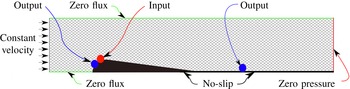
We consider a linear numerical simulation of flow over an idealized aerofoil followed by an infinite plate. The aerofoil consists of a circular body of radius
 $R$
and two straight segments joining at the trailing edge (see Wallace & McKeon Reference Wallace and McKeon2012 for an experimental implementation). The Reynolds number based on
 $R$
is
 $Re=400$
, the radius
 $R=0.5$
and the chord length is 4.6 non-dimensional units; see figure 6 for a sketch of the flow configuration. With a unit inflow velocity, the viscosity is chosen to correspond to the inverse Reynolds number
 ${\it\nu}=1/Re$
. The flow domain is meshed by a two-dimensional unstructured grid of approximately
 $5\times 10^{5}$
nodes. First, a stable base flow is computed using a Newton iterative solver. Then, equations for the temporal evolution of perturbations
 $(u,v,p)$
around this base flow are formulated and spatially discretized using finite elements (in our case,
 $P_{2}{-}P_{1}$
Taylor–Hood elements). The pressure field is computed using the Uzawa algorithm with a Cahouet–Chabart preconditioner (see Glowinski Reference Glowinski2003). The time discretization is semi-implicit based on a second-order backward-differentiation scheme. We choose a time step of
 ${\rm\Delta}t=0.003$
for the simulations. Data sequences generated by the simulations are extracted with a time step of
 $\text{d}t=0.075$
, before being subjected to the identification algorithms. The length of the sampled data is
 $N=1500$
, and the entire measurement sequence is used in the identification algorithms. Two simulations are performed: the first contains an upstream source of noise (one radius
 $R$
upstream of the leading edge) that creates fluctuations in the flow field which are detected by both sensors; in the second simulation, a broadband pseudorandom binary signal (PRBS) is applied to the input which mostly affects the downstream sensor. At the downstream sensor location, a shear-stress signal (as feasible in a physical experiment) is collected. Artificial measurement perturbations are added to the downstream sensor, using a white Gaussian noise with the same variance as the noise-free signal variance (i.e. we consider a 100 % noise contamination); this choice is intended to simulate adverse experimental conditions and, at the same time, challenge the robustness of the system-identification algorithm. We would like to point out, however, that the amount of noise contamination has little influence on the perturbation approach, and an uncontaminated output/sensor signal would have produced nearly identical results. All identified nominal transfer functions will be found using the ARMarkov identification algorithm with the set of parameters
 ${\it\mu}=200$
,
 $n=20$
and
 $N=1500$
. Based on the given noise standard deviation, the standard deviation of each Markov parameter is estimated using the uncertainty-propagation algorithm given by (3.11). Finally, exact transfer functions are also identified from longer noise-free data signals (with
 $N=4000$
). These latter signals are assumed to be unobtainable in realistic experiments; they are computed here solely for a performance evaluation of the uncertainty-propagation algorithm.
Numerical domain and boundary conditions for the case of flow over an idealized aerofoil.

With the nominal transfer function and the different controller transfer functions known, it is then possible to estimate the performance and stability of a given controlled system. The following subsections focus on two control set-ups: a feedback and a feed-forward configuration. It will be shown that the exact performance and stability are quite different from the nominal values, and that this difference is well predicted by the uncertainty-propagation technique.
4.1 Feedback control
We first consider a feedback configuration for flow over the idealized aerofoil. The developed framework applies to the block diagram shown in figure 3(a) where, in the present case,
 $y$
denotes the signal from the downstream sensor and
 $u$
stands for the upstream control input. From the realistic (i.e. noise-contaminated) data sequence, the nominal transfer function (Markov parameters) is identified using the ARMarkov/LS identification algorithm. The number of identified Markov parameters is set to
 ${\it\mu}=200$
, which is approximately 1.4 times the AIC value of
 ${\it\mu}=144$
. The nominal system together with the noise standard deviation then provides an estimate of the standard deviation of the identified Markov parameters. This latter standard deviation can be interpreted as uncertainty bands about the nominal transfer function.
For demonstration purposes, we assume a proportional feedback controller with
 $K=0.025$
. The stability of the closed-loop system is determined by the distance of the OLTF
 $G_{0}K$
from the point
 $-1$
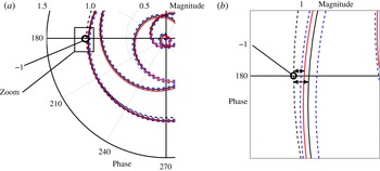
; see (2.17). Figure 7(a,b) show the Nyquist plots of the exact OLTF, the nominal OLTF and the uncertainty bounds associated with twice the standard deviation at each frequency. These bounds correspond to a confidence interval of 95 %, i.e. in only 5 % of cases does the real OLTF fall outside these bounds. Furthermore, the nominal transfer function of the controlled system shows a gain margin of
 $\text{GM}^{+}=0.033~\text{dB}$
, which overestimates the real gain margin by more than 40 % (
 $\text{GM}^{+}=0.023~\text{dB}$
). Our uncertainty-propagation algorithm gives estimates for the gain margin of more than
 $\text{GM}^{+}=0.017~\text{dB}$
with a probability of 95 %, and more than
 $\text{GM}^{+}=0.025~\text{dB}$
with a probability of 68.2 %. According to the same algorithm, the standard deviation of the gain margin is approximately
 ${\it\sigma}_{GM^{+}}=0.008~\text{dB}$
. In contrast, the singularity at
 $-1$
is nearly four standard deviations away from the nominal transfer function, which – according to the gain margin criterion and under the assumption of Gaussian noise – suggests that in only 0.1 % of all cases should we expect an unstable feedback-controlled system. A similar comparison may be performed using the phase margin: the nominal margin is
 $\text{PM}=29^{\circ }$
, the exact phase margin is
 $\text{PM}=21^{\circ }$
, while the
 $95\,\%$
-likelihood margin is determined as
 $\text{PM}=13^{\circ }$
.
(a) Nyquist plot of the OLTF. The red lines show the exact value and the black lines show the nominal value; the 95 %-likelihood bounds around the nominal value are given by dashed blue lines. (b) Magnified detail of the OLTF in (a) near the point
 $z=-1$
, with arrows showing the nominal and real gain margins. The dashed black line indicates the unit circle.

In this feedback control example, compared with the nominal transfer function, the real transfer function tends to overestimate the stability margins of the closed-loop system. The uncertainty-propagation technique allows a quantitative estimation of the error bounds, which results in a more realistic estimation of these margins.
4.2 Feed-forward control
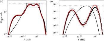
In feed-forward control applications, the control performance is often measured by the maximum magnitude of the CSTF. In this case, the input signal comes from the upstream sensor (see figure 6). As before, this CSTF can be estimated with the nominal identifications and compared with the real transfer function. Figure 8(a,b) shows the transfer function of the exact system without control, the nominal controlled system and the exact controlled system. This time, the performance of the controller seems to be positive (note the reduction of the maximal amplitude) with the nominal estimation. However, a closer look reveals that the real system behaves worse with control than without. This can be predicted using the 95 %-uncertainty bounds which show the probable lack of performance of the controlled system.
(a) Bode diagram of the uncontrolled system (black line), the nominal CSTF (black thick line), and the exact CSTF (red); the error bounds around the nominal CSTF are shown by black dot-dashed lines. The maximum amplitude of the uncontrolled system is represented by a dashed horizontal line. (b) Magnified view of (a) for a limited frequency range.

5 Conclusions
The identification error due to measurement uncertainty can have an important effect on the stability margins and performance bounds of any data-based controller. In this study, an uncertainty-propagation technique has been developed and applied to two types of control architecture: feedback and feed-forward control. In both cases, the nominal prediction overestimates either the controller performance or the stability margins. When input-data uncertainty is taken into account, more accurate predictions can be made. Even though uncertainty propagation may be treated via Monte Carlo analysis, the related computational costs are often prohibitive. In contrast, a linearization of the identification algorithm provides statistical information about the identified transfer function, requiring only a single experiment and thus overcoming the previous computational bottleneck. Estimating a priori the performance and stability characteristics of a given controller, using the data sequences from which the controller has been designed, may lead to a better design of control strategies. In fact, controllers are commonly built to be optimal in the nominal sense. Being able to give a robust definition of optimality with respect to uncertainty should allow the construction of control set-ups that are more relevant for implementation in experiments or more suited for the control of flows under realistic conditions.
We have restricted our analysis to linear models and a specific system-identification technique (ARMarkov/LS). Linear techniques still dominate the bulk of flow-control applications, as the evolution and manipulation of small-amplitude disturbances about steady or quasisteady states are common and widespread in a wide range of flow configurations (see, e.g., Rathnasingham & Breuer Reference Rathnasingham and Breuer2003; Juillet, McKeon & Schmid Reference Juillet, McKeon and Schmid2014). It should also be mentioned that even in the presence of an underlying nonlinear system, which has to be identified using nonlinear system-identification techniques as well as nonlinear control techniques, the influence of small disturbances in the processed data and their impact on control performance can still be analysed within a linear framework, i.e. by a sequence of linearizations. Special techniques developed for (nonlinear) Wiener or Hammerstein systems are conceivable for replacing the linear identification methods used in this study. Similarly, our choice of system-identification algorithm does not impose limitations on the applicability to other techniques, such as observer/Kalman filter identification (OKID); the perturbations in the identified Markov parameters due to uncertainty and noise in the processed data sequence will yield very similar expressions and only differ in the shape of the underlying frequency response model. Subspace identification techniques, which directly identify a state-space model and bypass the discrete transfer function, would require more notable changes to the present procedure; an effort in this direction is left for a future endeavour.
Appendix A. Transfer functions for linear time-invariant systems
Three different models have been introduced in § 2.1. For the sake of completeness, we present the transfer functions of these models, which can be obtained by taking the
 $z$
-transform of the equivalent discrete-time models.
For the FIR model we obtain the transfer function
 $$\begin{eqnarray}G(z)=H_{0}+H_{1}z^{-1}+\cdots +H_{{\it\mu}-1}z^{1-{\it\mu}},\end{eqnarray}$$
with
 $H_{i}$
as the Markov parameters (discrete impulse response). The transfer function is simply a sum of monomials in
 $z^{-1}$
. Following the same procedure, the more complicated ARMA model yields the transfer function
 $$\begin{eqnarray}G(z)=\frac{M_{0}+M_{1}z^{-1}+\cdots +M_{n}z^{-n}}{1+N_{1}z^{-1}+\cdots +N_{n}z^{-n}},\end{eqnarray}$$
which represents a rational function in
 $z^{-1}$
to approximate the transfer function of the identified system. The third and final model, the ARMarkov model, has the transfer function
 $$\begin{eqnarray}G(z)=\frac{H_{0}+H_{1}z^{-1}+\cdots +H_{{\it\mu}-1}z^{-({\it\mu}-1)}+z^{-{\it\mu}}(Q_{0}+Q_{1}z^{-1}+\cdots +Q_{n}z^{-n})}{1+z^{-{\it\mu}}(N_{1}z^{-1}+\cdots +N_{n}z^{-n})},\end{eqnarray}$$
which also represents a rational approximation of the system response but, contrary to the previous ARMA model, contains the first
 ${\it\mu}$
Markov parameters
 $H_{i}$
explicitly.
Appendix B. Validation using Monte Carlo simulation
We will validate the perturbation framework introduced in the main text using Monte Carlo simulations. In particular, we wish to assess the dependence of the perturbative approach on the signal-to-noise ratio of the processed data. To this end, we introduce the parameter
 ${\it\gamma}$
, defined as
 ${\it\gamma}={\it\sigma}_{{\it\delta}y}/{\it\sigma}_{y}$
, measuring the standard deviation of the perturbations relative to the standard deviation of the unperturbed data. For efficiency reasons, we choose as our test case a system that can be solved quickly, yet still has the characteristics of a full-scale fluid system. In particular, the chosen system should produce data sequences reminiscent of many fluid systems: with a range of certain frequencies amplified by the flow, while other frequencies are damped, and with a delay between input and output signals mimicking advection.
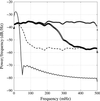
The power spectral densities of the different measurement disturbances: crosses denote the white noise, circles show the coloured noise 1, the dashed line displays the coloured noise 2. The spectrum of the noise-free output signal is represented by the solid line.

The selected test case consists of incompressible flow around a cylinder (
 $Re=40$
), modelled by the linear complex Ginzburg–Landau equation. An actuator is placed approximately half a radius upstream of the cylinder, and the sensor is located in the stable wake; both impose or provide signals of the normal-velocity component. The linear Ginzburg–Landau model equation is solved numerically using finite differences on a one-dimensional equispaced mesh of
 $N=100$
grid points. The relatively small dimensionality of the system facilitates the convergence of the Monte Carlo variance estimation. The flow behaves as a filter with delay, and the power spectral density of the output signal (given white-noise input) is plotted in figure 9 (solid line); it shows amplification of lower frequencies (around 25 mHz) and a strong damping of higher frequencies. The input sequence has been generated with a PRBS algorithm. A total of 500 noise-free numerical experiments have been performed, resulting in 500 independent noise-free input–output data sequences, with each sequence containing 1000 measurement points sampled at 1 Hz (i.e. approximately 50 times the characteristic time scale of the system). The length of each sequence represents 25 characteristic time units. This length and the sampling frequency are adequate to accurately identify the system behaviour (see § 2.2).
After establishing the baseline data sequences, we add noise to each of the 500 experiments. In general, three different approaches can be distinguished. The added noise could be (i) broadband and affect all frequencies nearly equally. Alternatively, it could be strongly coloured with (ii) higher amplitudes near the natural frequency of the system or (iii) higher amplitudes at higher frequencies that do not correspond to physically observed frequencies. Often, the characteristic frequency of the system can be estimated, which allows the application of low-pass filters to eliminate the noise for the third case. In the first two cases, low-pass filtering will not succeed in eliminating the noise components in the data. For this reason, we will focus on these cases.
Three different measurement contaminations will be considered: white noise and two coloured noise distributions with a pronounced amplitude near the characteristic frequencies of the system. Their power spectra are presented in figure 9 together with the output power spectrum. These noise spectra cannot be simply filtered and are likely to influence the values of the identified Markov parameters. Their noise-to-signal ratio
 ${\it\gamma}$
is set by choosing the noise amplitude. For each of the three noise spectra and for every considered noise-to-signal ratio, we compare the statistical information estimated by the Monte Carlo approach with the same information computed by the uncertainty algorithm of the main text. The mean standard deviation of the identified Markov parameter (mean(
 ${\it\sigma}_{H}$
)) is the objective for this test case; it has to be compared with the average of the Markov parameter value, which is 1. If
 $\text{mean}({\it\sigma}_{H})=10^{-2}$
, the variance error is estimated to be on average 1 % for each Markov parameter.
First, 500 noisy data sequences are used to estimate the standard deviation of the identified Markov parameters (the Monte Carlo approach). Then, one single input–output data sequence and the noise standard deviation are used to estimate the standard deviation of the identified Markov parameters (using the uncertainty-propagation approach). For the Monte Carlo estimation, each of the 500 perturbed input–output data sequences is used in the ARMarkov/LS identification algorithm, yielding the corresponding Markov parameters; from these 500 sets of Markov parameters, their means and standard deviations can easily be determined. For the uncertainty propagation, one arbitrarily perturbed data sequence is taken as input to the algorithm of § 3. Equation (3.11) produces the standard deviation of the Markov parameters based on the noise standard deviation, from which the mean can be computed. The parameters for the different algorithms are
 $N=1000$
,
 ${\it\mu}=400$
,
 $n=40$
, and
 ${\it\epsilon}$
is set to machine precision. The corresponding AIC is not given, since its value varies with each noise-to-signal ratio and each colour of noise. Figure 10 shows the results of the standard deviation estimates for each algorithm (Monte Carlo and uncertainty propagation) and for each noise-spectrum/noise-to-signal ratio.
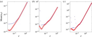
Monte Carlo (blue dots) and uncertainty-propagation (red squares) estimates of the standard deviation of the identified Markov parameters as a function of the noise-to-signal ratio
 ${\it\gamma}$
. (a) Measurement contamination by white noise; (b) measurement contamination by low-pass filtered noise 1; (c) measurement contamination by low-pass filtered noise 2.

As can be deduced from figure 10, the three different noise spectra (measurement contaminations) affect the standard deviation of the Markov parameters in a similar manner. Independent of the noise spectrum, the Monte Carlo and uncertainty-propagation approaches give identical estimates for high noise-to-signal ratios, thus validating the uncertainty-propagation algorithm for sufficiently high values of
 ${\it\gamma}$
. According to these experiments, accurate estimates of the standard deviation of the Markov parameters can be expected for noise-to-signal ratios
 ${\it\gamma}$
between
 $10^{-5}$
and 2 (very noisy signal). For low values of
 ${\it\gamma}$
(
 $\ll 10^{-5}$
), two reasons may explain the discrepancy between the Monte Carlo results and the uncertainty propagation. First, the standard deviation may be influenced by round-off errors which become important at
 $10^{-8}$
due to the square root dependence of the standard deviation. Second, with only 500 samples available, the Monte Carlo algorithm may only be converged up to
 $10^{-6}$
. In any event, realistic data sequences taken from fluid systems are rarely contaminated by noise of less than 0.001 %.
This simple test case illustrates that uncertainty propagation provides accurate and valuable estimates of the Markov-parameter variance error for realistic noise-to-signal ratios.