Introduction

In general circulation models (GCMs) the simulation of Antarctic sea ice for the present climate and global warming scenarios shows large climatic impacts of changes in the sea-ice area. However, large differences exist between the models in the simulation of the sea ice and its changes (Grotch, Reference Grotch1988). Treatments of sea ice in atmospheric GCMs have been relatively simple, without prognostic formulations of ice dynamics, drift and open-water fractions (Schlesinger and Mitchell, Reference Mitchell, MacCracken and Luther1985). Conversely, the simulations of the Antarctic sea ice using more sophisticated treatments of dynamics and thermodynamics have been applied to limited-area studies only, or have involved other simplifications, such as the use of prescribed atmospheric forcings (e.g. Parkinson and Washington, 1870; Hibler and Ackley, Reference Hibler, III. and Ackley1983; Parkinson and Bindschadlcr, 1984; Stössel and others, 1989). Our objective here is to include a more realistic formulation of sea ice in the global GCM to improve the simulations of the Antarctic sea ice.

There is a need to incorporate more advanced treatments of sea ice into the atmospheric GCMs with a coupled surface ocean, in order to generate prognostic determination of heat and moisture fluxes, sea-ice area (including the open-water fraction) and sea-ice advection. For coupled models to perform satisfactorily, it is necessary for the atmospheric GCM to reproduce adequately the present distribution of surface temperature, pressure and winds around the Antarctic. The present work builds upon the GCM studies of Simmonds and Budd (Reference Simmonds and Budd1990) who examined the sensitivity of a GCM to changes in the open-water fraction within the Antarctic sea-ice area. They found that the simulated mean surface-pressure pattern from the GCM for the “perpetual July” was in reasonable agreement with observations when the prescribed sea-ice concentration was also similar to that observed for July.

Our longer term aim is to simulate the annual cycle of sea ice and climate in a coupled system with a mixed-layer ocean and prognostic sea ice including the open-water fraction. It is also desirable for the sea-ice model in the GCM to be computationally efficient and to have high enough resolution to adequately represent changes in the sea-ice area. The GCM used for the sea-ice model outlined here is based on the Melbourne University spectral model (R21 × L9 version 5.3, used by Simmonds and Budd, Reference Simmonds and Budd1990).

The GCMs used to simulate the global climate and the response to a doubling of CO₂, tus described by Grotch (Reference Grotch1988), used motionless “slab oceans” with prescribed ocean “flux corrections” so as to give the observed sea-surface temperature distribution for the present climate. Similarly, prescribed ocean heat fluxes were used under the sea ice. Our objective is to include a wind-driven ocean with a variable mixed-layer depth, in conjunction with the dynamic-thermodynamic sea-ice model, so that the ocean advective, as well as storage, heat fluxes are computed rather than prescribed.

The Antarctic sea-ice changes develop as a result of a relatively fine balance between large atmospheric and oceanic heat fluxes. One of the problems so far has been to determine how the relatively thin and open Antarctic pack ice in winter can be sustained under large heat fluxes to the atmosphere. This paper addresses that problem.

We first examine the ocean mixed-layer dynamics and thermodynamics based on observations. We then briefly outline the essential features of the sea-ice model, following on from the work of Parkinson and Washington (Reference Parkinson and Washington1979) and Flato and Hibler (Reference Flato and Hibler, III.1990). Finally, we consider the atmospheric heat fluxes and some July sensitivity simulations of sea-ice thickness and concentration.

The GCM computes winds, heat fluxes, surface temperature, evaporation and precipitation, which influence the sea-ice and surface-ocean model. The sea-ice and

Fig. 1.

Pattern of Southern hemisphere monthly mean ocean-drift vectors for July from the Melbourne University 5° × 5° data set described by Budd (Reference Budd1986).

ocean parts of the model compute the ice thickness and concentration, as well as heat flux components required for the surface temperature, which provides the surface boundary condition for the atmosphere.

The Mixed-Layer Ocean Model

Fully coupled atmosphere-ocean models are still under development and, so far, have presented difficulties in simulating the full annual cycle of the observed atmosphere-ice-occan system. Here we use an upper mixed-layer ocean for thermodynamics, including horizontal advection for the present climate, derived from the present mean ocean drift as described by Budd (Reference Budd1986). It is assumed that the deep-ocean circulation and the circulation of the lower part of the mixed layer are controlled largely by the ocean bed topography, the mean wind forcing over the seale of a month and, to a smaller degree, the ocean geostrophic flow related to the deep ocean density structure. The surface ocean flow is assumed to be driven by both the surface wind on a daily time seale and a steadier deeper ocean flow.

The mean ocean-drift data set, described by Budd (Reference Budd1986), supports these assumptions. This data set was derived from the drift of buoys and icebergs. Observed drift data were used to construct a data set of mean monthly ocean surface drift rates for the Southern Ocean on a 5° lat. × 5° long. grid. This data set was then combined with that of Meehl (1980) to give a global coverage. Mean ocean current vectors for July, derived from the set, are shown in Figure 1. The integrated displacement from the currents over a six month period is illustrated in Figure 2. These displacements also depict the ap-

Fig. 2.

The pattern of mean six month surface, ocean-drift displacement (thick lines) from the gridded data set is shown superimposed on the 3000 m bed topography (thin dashed lines). The dotted line shows the average ice extent for September.

proximate movement of the sea ice during winter. The asymmetry of the mean maximum ice edge for September strongly reflects the influence of the ice drift.

The basis of the assumption above, that the monthly mean surface drift corresponds closely to the deeper ocean flow, is supported by the close correspondence between the monthly mean drift of the icebergs and the drifting buoys as shown by Tchernia and Jeannin (1983), Hamley and Budd (Reference Budd1986) and Allison (Reference Allison1989). On the shorter time scales, the buoys show much more reaction to the transient wind variations than do icebergs. The pattern of ocean drift also shows close similarity to the mean surface geostrophic wind, particularly at high latitudes, as depicted by the surface pressure pattern for July (Fig. 3). A close relation between the buoy drift and mean geostrophic wind was also obtained by Allison (Reference Allison1989). The following wind-driven drift formulation captures the most important aspects of these observations by including mean and transient components of the ocean and wind velocities.

The magnitudes of the mean ocean-drift velocity (V_o) from the data set were found by Budd (Reference Budd1986) to be related to the atmospheric surface geostrophic wind (V_O) by the approximate relation

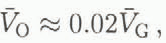
where the over-bar denotes the one month average.

To provide wind-driven drift relation which gives the present observed drift rates, and takes account of other effects such as topography and the deep ocean flow, the following relation is used for the velocity vectors:

Fig. 3.

The mean surface pressure for the southern hemisphere in July, from Schutz and Gates (Reference Schutz and Gates1974), shows a close relation to the pattern of mean ocean drift of Figure. 1.

where λ and V̄_D are determined for each grid point to provide a close matching between the present ocean drift and the geostrophic surface wind on a monthly-mean basis. The average value of A over all grid points gives a relation similar to Equation (1).

For the transient, unimpeded drift (“free” drift) of the sea ice and ocean surface (V_i) the following relation is used:

where V_G is the instantaneous atmospheric geostrophic wind. This relation allows the ice drift, when unobstructed, to respond to local transient wind changes. However, on the long term average for the present climate, the ice drift tends to follow the pattern of the observed mean ocean drift. For climatic change studies it is assumed that the deep-occan density structure and flow are less affected over the time seales under consideration. Such changes can only be addressed by deep global-ocean circulation models which can accurately simulate the present deep-ocean circulation and the physical processes involved in the changes, cf., for example, Mikola-jewicz and Maier-Reimer (Reference Mikolajewicz and E.1990).

Thermodynamics, Ice Thickness and Ocean Storage

The surface fluxes are computed from the GCM over the ocean and sea ice as described by Simmonds and Budd (Reference Simmonds and Budd1990). For grid boxes containing sea ice, separate heat balance conditions apply over the ice and over the open-water parts, which together constitute the balance over the grid box as a whole. The model of Simmonds and Budd (Reference Simmonds and Budd1990) determines the mean surface temperatures and fluxes over the grid box as well as those of the different surfaces. In particular, the GCM calculates the components of the surface heat balance which govern the atmospheric exchange with the ocean and sea ice. These heat balance components consist of the net radiation, N, the sensible heat flux, S, and the latent (evaporative) heat flux, L, (all upwards positive). Over the ice-covered water, the difference between the total flux to the atmosphere (N + S + L) and the flux from the ocean provides the thermodynamic balance which determines the ice growth or melt.

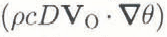
For ice-frce areas, the ocean heat storage change for the surface mixed layer is computed from the relation for an incompressible fluid

where ρ is the water density, c its specific heat, D the effective mixed-layer depth, θ the mean mixed-layer temperature, t time, V_o the mean ocean-surface layer drift rate and F₀ the exchange with the deeper water.

The deep-ocean heat flux, F₀ is a small residual term which is not accurately known from observations, and so is set to preserve the heat balance for the present climate. It should be noted that the conventional “flux correction” used in GCMs with a “slab ocean” (cf. Schlesinger and Mitchell, Reference Mitchell, MacCracken and Luther1985), also includes effects of the advection term

and in some cases also effects of varying D in the storage term

The effective mixed-layer depths used here have been taken from observations of the annual cycle of the temperature depth profile (e.g. Levitus, 1984; Allison, Reference Allison1989). When the surface ocean reaches freezing point (≈ −1.8°C), the additional heat loss is converted into ice growth. The model ice thickness needs to simulate the observed ice thickness for the annual cycle. The variation in ice thickness in the fast-ice zone around the coast through the year, where measurements are available, has been summarised by Budd (Reference Budd1982). For the open pack, fewer observations are available and the effects of ice movement and open-water fraction need to be taken into account. A compilation of the observed mean ice thickness at maximum is given by Budd (Reference Budd1986) and the variation through the year by Budd (Reference Budd1982).

Over the pack ice with open water, part of the ice growth goes to increase the ice thickness, and part to increase the ice area. To model this requires some assumptions. We make the following:

• • Well-mixed ocean surface layer assumption: it is assumed that, in the presence of ice, the upper mixed-layer of the ocean is continually well-mixed thermally and is uniformly at the freezing point. Any gain or loss of heat through the ice or open-water fraction is assumed to be converted into latent heat by freezing or melting of ice uniformly over the area.

• • Partitioning of ice thickness and area changes assumption: although the heat exchange over the open-water fraction may be much larger than that over the ice fraction, the well-mixed ocean assumption provides that the latent heat changes can be assumed to result in a uniform ice-thickness change over both areas. This process corresponds to the accumulation of frazil ice under the old ice floes from heat loss through the open water along with freezing within the open-water area.

• • Redistribution of thin ice (pancaking) assumption: only an average ice thickness over a grid box is carried in the model. It is assumed that during ice growth the new ice formed over the open-water fraction is redistributed to the edges of the existing ice to increase the ice area while maintaining ice of uniform average thickness. In practice, this occurs to a certain extent through the dynamic interaction between ice floes which compresses the new, thin ice to the edges of the existing floes. This is analogous to the processes involved with the formation of “pancake” ice on a smaller seale. A similar assumption is adopted for the melting processes.

These assumptions, along with the dynamics, provide the basis for the model to simulate the pattern of mean maximum ice thickness, given by Budd (Reference Budd1986), and the mean ice concentration shown, for example, for September, given by Zwally and others (Reference Zwally, Comiso, Parkinson, Campbell, Carscy and Gloersen.1983).

Ice Concentration Changes

Changes in ice concentration result from the dynamics through advection, convergence or divergence, and through the thermodynamics, which changes the relative ice and open-water areas.

The change of ice concentration (C _i) with time is then given by

where

represents the rate of ice-concentration change from the thermodynamics and V_i is the ice-drift vector.

We now consider some different forms of the sea-ice dynamics and rheology. Sensitivity studies are being carried out to examine the performance of different formulations, following Parkinson and Washington (Reference Parkinson and Washington1979), Hibler (1979) anil Flato and Hibler (Reference Flato and Hibler, III.1990). The simplest version which gives a reasonable approximation for the Antarctic sea-ice distribution considers the pack as a set of solid loose slabs which moves with the surface ocean in free drift until compacted. This formulation corresponds to the Flato and Hibler (Reference Flato and Hibler, III.1990) “incompressible cavitating fluid”. The additional requirements for compressible sea-ice pack are discussed in the following section.

Solid ice slabs with zero resistance to tension or shear (incompressible cavitating fluid)

The formulation for the dynamics has been given by Flato and Hibler (Reference Flato and Hibler, III.1990). They indicate that their formulation is an improvement on that of Parkinson and Washington (Reference Parkinson and Washington1979), in that it conserves momentum and, for the Arctic, does not tend to stagnation in confined regions. For the Antarctic this defect is not so pronounced.

Most Antarctic sea ice is first-year ice with a substantial open-water fraction. Around the coastal region some compact ice occurs, often with rafting several annual layers thick. However, this represents only a relatively small fraction of the total area, and is small relative to the grid seale of the model.

The main features of importance from the sea-ice model for the atmosphere are the relative areas of ice and open water. The solid-slab hypothesis allows ice compaction to 100% of ice concentration without thickness change, when obstructed and shearing, or divergence under wind forcing without additional ice resistance. It is found that this assumption leads to realistic ice concentrations around the continent (similar to that shown in Fig. 6) with generally higher concentrations around the coast and decreasing outwards towards the open-water areas. The solid-slab assumption, however, does not simulate the effect of ice-thickness increases due to compression with rafting and over-lapping of the ice floes, as observed in some parts of the Weddell Sea (Ackley, Reference Ackley1979) and near the coast off East Antarctica (Jacka and others, Reference Jacka, Allison, Thwaitcs and Wilson1987). To address these processes a simple compression rheology is introduced.

A SIMPLE COMPRESSION RHEOLOGY

A scheme for modelling sea-ice rheology using a variable ice-thickness distribution has been given by Hibler (Reference Hibler, III.1980). Here we use a simpler formulation which considers only an average ice thickness (h) over a grid area. The formulation is similar to the “compressible cavitating fluid” scheme of Flato and Hibler (Reference Flato and Hibler, III.1990) and has the following characteristics:

• • Tension or shear are not resisted in the absence of net convergence.

• • Compression is resisted beyond a critical ice concentration, currently set at (C_i) ₁ = 90%, (cf. Flato and Hibler, in press).

• • The rate of horizontal compaction of the floes is reduced beyond C_i = 90% by linearly reducing and redistributing the components of ice velocity (u,v), following Flato and Hibler (Reference Flato and Hibler, III.1990), with C_i reaching an order of magnitude reduction when C_{i 2} = 98%.

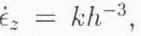
• • Ice volume is preserved through continuity by allowing compression beyond C_i = 100% to convert ice-area decrease from convergence into ice-thickness increase, i.e. the vertical strain rate

  
  is related to the horizontal strain rates by
  

  (6)
  or, in terms of change of ice thickness, h,
  

• • The rate of compression is taken to decrease, with increasing thickness beyond h₀ = 0.1 m, by the relation

  
  where k is chosen to correspond to the value of compression at C_i = 98%. This relation considers the ice-resistance stress to be distributed uniformly over the thickness, for given body forces (provided by the surface stresses). Since the deformation rate of ice in secondary or tertiary flow varies as the third power of stress, the compression rate of the pack is taken to decrease similarly with ice thickness.

The above formulation relates ice motion and convergence directly to the wind and current forcing, decreasing initially with increasing compaction, and then more strongly with increasing ice thickness. The prescribed constants, (C_i)₁, (C_i)₂, h₀ and k are not well known, a priori, for an arbitrary ice pack, but are all capable of being set to match observations. Modelling-sensitivity studies are being carried out to test the model response to a range of settings.

Heat Fluxes and Ice-Growth Rates

Strong coupling exists between the atmosphere and sea ice during the Antarctic winter. The open-water fraction of the sea-ice cover strongly influences the heat flux and atmospheric circulation, which in turn controls the ice growth and concentration. Parkinson and Cavalieri (Reference Parkinson and Cavalieri1982) showed how the atmospheric circulation influences the sea-ice distribution. Equally, the sea-ice distribution influences the atmospheric surface pressure field through the surface heat fluxes. Changes in zonal mean surface heat fluxes in the GCM, from prescribed increases in the sea-ice open-water fraction, are shown in Figure 4 for July. For 100% ice cover, heat losses from the ocean north of the sea-ice zone exceed 190 W m⁻² with negligi

Fig. 4.

Total zonal aerage energy flux (W m⁻²) into the atmosphre from the surface as a function of latitude for different open-water fractions prescribed in the GCM simulation for July.

ble loss over the sea-ice zone. For 50% ice cover the corresponding values are below 130 W m⁻² for the ocean north of the sea ice and about 70 W m^x−2 averaged over the sea-ice zone. The heat loss over the sea-ice zone amounts to about half from sea-ice growth and the remainder from ocean exchange. The latter is largely associated with the deepening of the freezing mixed layer into warmer water below. Some components of the ocean and sea-ice heat balance through the year are given in Table 1.

There is a rapid change in heat loss going from open-water fractions (f_w) of 5 to 50%, which span the bulk of the area of the observed concentration in July. The distribution of total heat flux from the model run for f_w = 50% is shown in Figure 5. The changes in sur-

Fig. 5.

The distribution of total heat flux from the surface to the atmosphere for the GCM July simulation, with 50% open water in the sea ice. Contours at 50 W m⁻² heat flux.

Table 1.

Mean ocean-sea-ice heat balance elements, θ̅ = mixed-layer temperature, D̅ = effective mixed-layer depth, H̅ = change in ocean heat storage,

= change in ice thickness, C_i = ice concentration, and L_i = latent heat storage

Table 2.

Mean heat balance elements over sea-ice zone for different prescribed ice concentrations (C_i) in the July GCM simulations

face temperature and various components of the heat flux with ice concentration are shown in Table 2. The atmospheric temperatures and surface heat flux are likewise important factors in determining the ice-growth rate and changes of ice concentration. These processes have been studied in the interactive, coupled model by sensitivity studies.

Sensitivity Studies with the Coupled Atmosphere Ice-Ocean Model

Sensitivity studies have been carried out for July, starting with various initial ice concentrations and ice thicknesses. The model shows reasonable stability and yields simulated growth rates which compare favourably with observations. The concentration distribution also evolves well, including reasonable drift rates.

Fig. 6.

Sea-ice concentration generated by the coupled GCM sea-ice model for 90 days of July radiation, starting with ice thickness 0.5 m, concentration 70%, and with prescribed oceanic heat flux of 40 W m ⁻². Contours at 0.3–0.8 concentration.

An example of the ice concentration generated from a model sensitivity run is shown in Figure 6. In this case, the GCM was used for a simulation of July conditions for 90 days. The initial ice thickness was 0.5 m and the initial concentration was 70%. The prescribed ocean flux under the ice was 40 W m⁻². The concentration evolved to above 80% around the coast, decreasing to less thiin 30% near the edge. This pattern shows some similarity to the results from the satellite observations given by Zwally and others (Reference Zwally, Comiso, Parkinson, Campbell, Carscy and Gloersen.1983), with greater extent in the regions of the Weddell and Ross sea gyres and near 90° E. A similar pattern is found for the ice thickness shown in Figure 7. The simulated ice thickness varies from about 2.5 m in the Ross and Weddell seas to an average of about 1 m over a large part of the area, decreasing quickly to less than 0.3 m near the ice edge. In general, the pattern is similar to the results compiled from observations by Budd (Reference Budd1986), although the thickness off the coast of East Antarctica appears excessive.

Fig. 7.

The resulting sea-ice thickness distribution for the same conditions as Figure 6. Contours 0.3 to 2.5 m.

Fig. 8.

Change in ice concentration (a) and ice thickness (b) for different July simulations with the coupled GCM sea-ice model starting with initial concentrations (50, 70%), ice thickness (0.5, 1.0m) and applied oceanic heat fluxes 40, 80 W m⁻².

The simulations show that the effects of an initial, large perturbation can persist over months, suggesting appreciable persistence and feedback within the coupled system. This feedback and persistence may contribute to the strong interannual differences in the ice concentration and atmospheric circulation described by Parkinson and Cavalieri (Reference Parkinson and Cavalieri1982).

An example of the changes in thickness and concentration from initial prescribed conditions is shown in Figure 8. The rates of ice growth and change in concentration are shown for two different initial ice thicknesses (0.5 and 1 m) and ice concentrations (50 and 70%) and for the prescribed heat fluxes of 40 and 80 W m⁻².

The initial ice concentration made only a small difference to the ice-growth rate and, over time, the mean concentration tended to a common value of about 77%, close to that observed. The time required for the approach to the common concentration shows that large initial anomalies can persist for several months. The initial ice thickness (above 0.5 m) also did not affect the growth rate greatly.

The specification of ocean heat fluxes from 40 to 80 W m⁻² produced growth rates which span the observed range. The sensitivity studies indicate that ocean fluxes in the range of 50–x60 W m⁻² provide a reasonable match to observations. It can be seen from Tables 1 and 2 that these ocean fluxes are compatible with the fluxes from ocean storage, sea-ice growth and the total heat loss to the atmosphere.

Similar sensitivity studies for summer simulations have been carried out, which show the rapid retreat of the sea ice comparable with the observed changes. The results of the wide range of sensitivity studies in progress indicate encouraging performance of the coupled model in simulating the present climate and as a diagnostic tool to investigate the different components of the climate system in the sea-ice zone. The sea-ice part of the model is efficient and quick to compute, adding less than 1% to the computation time of the GCM. The coupled model appears to be stable, but allows for feedback and persistence. Experiments are now underway, using the full annual cycle, to study the simulation of the present climate including prognostic sea-ice characteristics and their responses to climatic changes.

Conclusions

The distributions of Antarctic sea-ice concentration and thickness have been successfully modelled interactively with a global general circulation climate model.

• • Sensitivity studies with the model show that the relatively low winter sea-ice concentration (averaging about 76%) and thin ice (averaging about 1 m) are compatible with high heat fluxes to the atmosphere (about 100 W m⁻²).

• • The source of the high winter oceanic heat flux is primarily from the deepening and mixing of the freezing mixed layer into warmer water below, as given in Table 1.

• • The low Antarctic ice concentration in winter is maintained by a balance between the divergent atmosphere ocean forcing and the thermodynamic new ice growth.

• • From the summer simulation results (not presented here) the absorption of heat through the large open-water fraction is found to be a major factor in the rapid retreat of the ice.