2.1. Description of the IRS-DC pension model

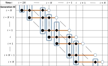
Figure 1 provides a schematic illustration of our pension model. The pension fund covers N overlapping working generations in each operating year (e.g., $N = 40$ ). The pension fund is fully funded. For simplicity, we assume that each generation consists of one hypothetical participant. Let $t \geqslant 0$ denote the time, with the unit being 1 year. We assume that the fund starts at time $t = 0$ with N initial generations.

Figure 1.

Schematic illustration of the pension model. The horizontal axis indicates time t and the vertical axis generation identifiers. For each generation, the black and white circles indicate the time points when that generation joins and retires from the pension fund, respectively; the orange line indicates the duration of the participation in the fund. For example, the generation i joins the fund at time $t = i-N$ and retires at $t = i$ . For each time point, the blue box indicates the current participants of the pension fund, and black diamonds indicate those participants (only shown for the generations displayed in the figure). For example, at time $t = i-1$ , the generations $i, i + 1, \dots, i+N-1$ are participating in the fund.

2.1.1. Generation identifier

We use an integer $i \in \mathbb{N}$ as the identity of the generation who retires at time $t = i$ (see Figure 1). Namely, the generation i joins the fund at time $t = i- N$ and leaves the fund at time $t = i$ ; thus, this generation is in the fund for N years. Using this notation, we can define the set of all the working generations in the fund at any time point $t \geqslant 0$ as:

\begin{equation*} I_{w}(t)\;:\!=\;\{i\vert i= [t] + 1,\ [t] + 2,\ \dots,\ [t] + N \}, \end{equation*}

where [t] denotes the integer part of t (e.g., if $t = 3.4$ then $[t] = 3$ ; if $t = 3$ then $[t] = 3$ ).

2.1.2. Financial market and pension asset dynamics

We consider a financial market where there exist two investment opportunities: a risky asset (e.g., a stock) and a risk-free asset (e.g., a bank account or a bond), denoted by S(t) and F(t), respectively. Specifically, we consider the Black–Scholes market, where S(t) is driven by a diffusion process with constant drift $\mu > 0$ and volatility $\sigma > 0$ , while F(t) develops at a risk-free rate $r > 0$ such that $\mu > r$ :

(2.1) \begin{align} {\textrm{d}}S(t)=\mu S(t){\textrm{d}}t+\sigma S(t){\textrm{d}}Z(t),\quad S(0)=1; \end{align}

(2.2) \begin{align} {\textrm{d}}F(t)=r F(t){\textrm{d}}t, \quad F(0)=1, \end{align}

where Z(t) is a standard Brownian motion under the real-world probability measure.

Let A(t) denote the asset of the pension fund at time t, with $A(0) > 0$ being the initial asset. For simplicity, we assume that the fund invests a constant fraction $\pi \in [0,1]$ of the pension asset A(t) in the stock S(t) and the rest $1-\pi$ in the risk-free asset F(t); thus, we can write the dynamics of the pension asset as:

(2.3) \begin{equation} {\textrm{d}}A(t)=\frac{\pi A(t)}{S(t)}{\textrm{d}}S(t)+\frac{(1-\pi)A(t)}{F(t)}{\textrm{d}}F(t), \quad\pi\in[0,1]. \end{equation}

We assume that the fund is prohibited from from borrowing ( $\pi>1$ ) and short selling ( $\pi<0$ ).

At the beginning of each year $t = 0, 1, 2 \dots$ , each working generation pays a constant amount of contribution, $c > 0$ , to the pension fund. Since there are N working generations, the fund thus receives a total of Nc contributions at the beginning of each year. At the same time, the fund pays a lump-sum benefit to the generation t, who retires at time t.

The dynamics of the pension asset can thus be written as:

(2.4) \begin{align} {\textrm{d}}A(t)= A(t)(\pi(\mu-r)+r)\;{\textrm{d}}t+ A(t)\pi\sigma\;{\textrm{d}}Z(t), \quad A(0)=A_0,\quad t>0, \end{align}

(2.5) \begin{align} A(t)_+ = A(t) + N c - B_t(t), \quad t = 0, 1, 2, \ldots, \end{align}

where (2.4) is obtained by substituting (2.1) and (2.2) into (2.3), $A(t)_+ \;:\!=\; \lim_{\varepsilon \to +0} A(t+\varepsilon)$ denotes the right continuous limit, and $B_t(t)$ is the benefit paid to the generation t who has just retired and defined in (2.6) and (2.7) below (the double t notation of $B_t(t)$ is deliberate and its meaning will be clear shortly).

Therefore, the pension asset develops continuously over time $t >0$ , while there is a jump at each integer time $t = 0, 1, 2, \ldots$ (i.e., at the beginning of each year) when there are incoming and outgoing cash flows of Nc and $B_t(t)$ , respectively.

2.1.3. Individual accounts and retirement benefits

Like pure DC and notional DC plans, each participant (generation) in our IRS-DC pension fund has her individual account, which keeps track of her pension rights. It records her annual contributions and grows according to the indexation rate (2.11) defined below. The terminal value of the account at the time of retirement becomes the lump-sum retirement benefit.

More formally, let $B_i(t)$ denote the individual account of generation $i \in \mathbb{N}$ at time $t \in [i-N, i]$ , which starts from $B_i(i-N) = 0$ when this generation enters the fund at time $t = i-N$ . Then, we define its dynamics as:

(2.6) \begin{align} B_i(t)_+= B_i(t) + c, \quad \quad t = i - N,\ \ i - N + 1,\ \dots,\ \ i - 1, \end{align}

(2.7) \begin{align} {\textrm{d}}B_i(t)=B_i(t)g(t){\textrm{d}}t, \quad \quad i - N \leqslant t \leqslant i. \end{align}

where g(t) is the indexation rate at time t, defined in (2.11) below. Namely, the individual account $B_i(t)$ grows continuously from the entry time $t = i - N$ until retirement at $t = i$ according to the indexation rate g(t) as (2.7), while the account accumulates the annual contribution c at the beginning of every year as (2.6). The account value at the time of retirement $t = i$ , that is, $B_t(t)$ , is the retirement benefit of the generation i; see (2.5).

2.1.4. Indexation rate and notional liability

We now define the indexation rate g(t) that determines the growth rate of individual accounts as in (2.7), which in turn affects the pension’s asset dynamics in (2.5). To this end, following Bams et al. (Reference Bams, Schotman and Tyagi2016) and Donnelly (Reference Donnelly2017), we first define a notional liability of the fund as:

(2.8) \begin{equation} L(t) \;:\!=\; \sum_{i \in I_w(t)} B_i(t), \quad t \geqslant 0. \end{equation}

That is, we define the notional liability L(t) of the fund at time t as the sum of individual accounts $B_i(t)$ for the current working generations $i \in I_w(t)$ .

If there is no cash flow in (2.5), the solution to the asset process (2.4) is given by stochastic exponential, which is a classic result in financial mathematics (e.g., Karatzas and Shreve Reference Karatzas and Shreve1991, Chapter 5), as:

(2.9) \begin{equation} A(t) = A(0) \exp \left( \int_{0}^t \tilde{\mu} {\textrm{d}}s + \int_{0}^t \tilde{\sigma} {\textrm{d}}Z(s) \right), \end{equation}

where $\tilde{\mu} > 0$ and $\tilde{\sigma} > 0 $ are constants defined as:

(2.10) \begin{equation} \tilde{\mu} \;:\!=\;\pi( \mu -r) + r - \frac{1}{2} \pi^2 \sigma^2, \quad \quad \tilde{\sigma} \;:\!=\; \pi \sigma. \end{equation}

Following Goecke (Reference Goecke2013, Equation (5)),Footnote 1 we then define the indexation rate g(t) as:

(2.11) \begin{equation} g(t) = \tilde{\mu} +\theta\ln\left(\frac{A(t)}{L(t)}\right), \quad t \geqslant 0, \end{equation}

where $\theta > 0$ is a constant, $\tilde{\mu}$ is from (2.10), A(t) is the pension fund’s asset process (2.4) (2.5), and L(t) is the notional liability (2.8).

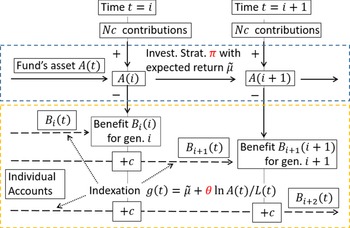
Figure 2 provides a schematic illustration of the cash flows in our pension model for two time points $t = i$ and $t = i + 1$ . In the following, let us take a closer look at the role of various important factors.

Figure 2.

Schematic illustration of the cash flows in our pension model for two time points $t = i$ and $t = i + 1$ . In the blue dotted box, A(t) denotes the pension fund’s asset, whose dynamics follow (2.4) and (2.5). In the orange dotted box, $B_i(t)$ , $B_{i+1}(t)$ , and $B_{i+2}(t)$ denote the individual accounts of generations i, $i+1$ , and $i+2$ , respectively, whose dynamics follow (2.6) and (2.7). At time $t = i$ , there is an incoming cash flow of Nc contributions from the N working generations, and an outgoing cash flow of the retirement benefit $B_i(i)$ for the generation i, who retires at time $t = i$ ; see (2.2). This retirement benefit is determined by the individual account $B_i(t)$ , which accumulates the annual contribution c at the beginning of each year and develops continuously according to the indexation rate $g(t) = \tilde{\mu} + \theta \ln( A(t)/L(t) )$ ; see (2.7). On the other hand, the asset process A(t) develops continuously according to the investment performance of the portfolio with the constant-mix strategy $\pi$ ; see (2.4). Each “ $+c$ ” represents the accumulation of the annual contribution in the individual account: at time t, the amount c is added to each of $B_{i+1}(t)$ and $B_{i+2}(t)$ .

2.2. Comparison with related pension models

We compare the IRS-DC model with related pension models in the literature. Goecke (Reference Goecke2013) studies the indexation rate (2.11) for the return smoothing in a self-financing pension plan. Goecke (Reference Goecke2013)’s model consists only of one generation, and there exists no cash flow of contributions and payments. The earlier work by Baumann and Müller (Reference Baumann and Müller2008) considers the indexation rate (2.11) where the risk-free rate r is used instead of $\tilde{\mu}$ . Our model is a continuous-time version of the discrete-time model of Bams et al. (Reference Bams, Schotman and Tyagi2016), which itself is an extension of the overlapping generations model of Gollier (Reference Gollier2008). Bams et al. (Reference Bams, Schotman and Tyagi2016) use the indexation rate in (2.11) but do not analytically study its use. Donnelly, (Reference Donnelly2017) considers a funded collective DC pension plan. Donnelly, (Reference Donnelly2017)’s model consists of fixed multiple overlapping generations, and there exists no new incoming generation. Donnelly, (Reference Donnelly2017) uses an automatic adjustment rule similar to Goecke, (Reference Goecke2013)’s (and thus ours) but is different in its concrete form.

Cui et al. (Reference Cui, De Jong and Ponds2011) consider a funded DB-based hybrid pension system that can adjust both benefits and contributions. Their pension model does not have individual accounts. The present value of base benefits and contributions are made equivalent ex ante, but there is no direct link between one’s actual benefits and contributions. Their model is DB-based in this sense. They use automatic adjustment rules for contributions and retirement benefits based on the funding ratio. Chen et al. (Reference Chen, Beetsma, Ponds and Romp2016) consider a hybrid pension plan as their second-pillar pension system, in which there exist individual accounts. They also use automatic adjustment rules for contributions and individual accounts’ indexation rates. While the adjustment rules of Cui et al. (Reference Cui, De Jong and Ponds2011) and Chen et al. (Reference Chen, Beetsma, Ponds and Romp2016) are conceptually similar to ours, they are different in their forms. For example, Chen et al. (Reference Chen, Beetsma, Ponds and Romp2016) use the “tangent hyperbolic adjustment function,” while our adjustment rule is based on the log notional funding ratio. Moreover, Cui et al. (Reference Cui, De Jong and Ponds2011) and Chen et al. (Reference Chen, Beetsma, Ponds and Romp2016) define the liabilities in a DB manner, taking into account future retirement benefits, while we define our notional liability in a DC manner, that is, as the sum of current individual account values. Again, our liability is notional, since the fund does not provide any promise on retirement benefits.

Automatic adjustment mechanisms have been implemented in real pension systems; see OECD, (2021, Chapter 2) for an overview. Notably, Sweden’s first-pillar notional DC pension system uses an automatic adjustment rule for the indexation rate of individual accounts Settergren (Reference Settergren2001). This adjustment mechanism is based on a notional funding ratioFootnote 2. and is conceptually similar to other rules discussed here (see e.g., Hagen Reference Hagen2013, Equations (6.2) and (6.3)). The Swedish first-pillar notional DC pension system defines its notional liability essentially in the same way as (2.8) (Settergren Reference Settergren2001, Equation (3)).Footnote 3

3.1. Dynamics of the log funding ratio

We start by analyzing the dynamics of the log funding ratio defined as:

(3.1) \begin{equation} \rho(t) \;:\!=\; \ln \left( \frac{A(t)}{L(t)} \right). \end{equation}

Goecke, (Reference Goecke2013, Proposition A.1) shows that $\rho(t)$ is an Ornstein–Uhlenbeck process under the assumption that there exists no cash flow. Baumann and Müller (Reference Baumann and Müller2008, Section 3.1) obtain a similar result, but again assuming no cash flow. Since our model involves explicit cash flows as in (2.5), these earlier results are not directly applicable. Nevertheless, we show here that $\rho(t)$ in our model is also an Ornstein–Uhlenbeck process if the time t is between integer time points. (Recall that cash flows in our model occur only at integer time points; see (2.5)). This result and intermediate derivations are later used for deriving further results, so we present them here for completeness.

Let $t_0 \in \mathbb{N}$ be an arbitrary integer time point, which corresponds to the beginning of a year. Then by (2.4), with $A(t_0)_+$ being the initial value after the contributions, the asset process A(t) for $t_0 < t < t_0 + 1$ is written as:

\begin{align*} A(t) = {{A(t_0)_{+}}} \exp\left( \int_{t_0}^t \tilde{\mu} {\textrm{d}}s + \int_{t_0}^t \tilde{\sigma} {\textrm{d}}Z(s) \right). \end{align*}

Notice the difference from the previous expression (2.9), which starts from $t = 0$ and holds only under the assumption that there exists no cash flow. Similarly, by (2.7), (2.8), and (2.11), the notional liability L(t) is given as:

(3.2) \begin{equation} L(t) = {{L(t_0)_+}} \exp \left( \int_{t_0}^t \tilde{\mu} {\textrm{d}}s + \theta \int_{t_0}^{t} \rho(s) {\textrm{d}}s \right). \end{equation}

Then for $t_0 < t < t_0 + 1$ , the log funding ratio $\rho(t)$ can be expanded as:

(3.3) \begin{align} \rho(t) &= \ln A(t) - \ln L(t) \nonumber \\[5pt] &= \ln {{A(t{_0})_+}} + \int_{t_0}^t \tilde{\mu}{\textrm{d}}s + \int_{t_0}^t \tilde{\sigma} {\textrm{d}} Z(s) - \ln {{L(t_0)_+}} - \int_{t_0}^t \tilde{\mu} {\textrm{d}}s - \theta \int_{t_0}^t \rho(s) {\textrm{d}}s \end{align}

(3.4) \begin{align} \hspace{-118pt} ={{ \rho(t_0)_+}} - \theta \int_{t_0}^t \rho(s) {\textrm{d}}s + \int_{t_0}^t \tilde{\sigma} {\textrm{d}} Z(s). \end{align}

The last expression is obtained because the two identical terms $\int_{t_0}^t \tilde{\mu}{\textrm{d}}s$ in (3.3) are canceled out. This is the result of the expected log return $\tilde{\mu}$ being used in defining the indexation rate (2.11), which in turn results in (3.2).

Equation (3.4) indicates that the log funding ratio $\rho(t)$ for $t_0 < t < t_0 + 1$ is an Ornstein–Uhlenbeck process with initial value $\rho(t_0)_+$ (e.g., Karatzas and Shreve Reference Karatzas and Shreve1998, p. 358), which can be written as:

(3.5) \begin{equation} \rho(t) = e^{ - \theta (t - t_0) } {{ \rho(t_0)_+}} + \tilde{\sigma} \int_{t_0}^t e^{ - \theta ( t - s ) } {\textrm{d}}Z(s), \quad t_0 \in \mathbb{N}, \quad t_0 < t < t_0 + 1. \end{equation}

This expression shows that $\rho(t) = \ln (A(t) / L(t))$ is mean-reverting in the sense that, irrespective of the value of $\rho(t_0)_+$ , it tends to 0 (in expectation) as t increases. In other words, the funding ratio $A(t) / L(t)$ tends to 1 as t increases.

3.2. Effects of the adjustment parameter on the funding ratio

Based on the expression (3.5), we next study how the adjustment parameter $\theta$ affects the dynamics of the log funding ratio $\rho(t)$ . We summarize key observations in the following proposition, the proof of which can be found in Appendix A.1.

Proposition 1 shows how the adjustment parameter $\theta$ affects the notional funding ratio $A(t)/L(t)$ and thus the stability of the pension fund. Point (iii) shows that a larger $\theta$ lets $A(t)/L(t)$ approach 1 more quickly and thus makes the fund more stable, while point (ii) indicates that a smaller $\theta$ makes the fund more volatile. Recall that the value of $\theta$ determines how strong the adjustment in the indexation rate g(t) works for the individual accounts $B_i(t)$ ; see (2.11). Therefore, a larger $\theta$ results in a stronger adjustment of the individual accounts $B_i(t)$ so that the notional liability $L(t) = \sum_{i \in I_w(t)} B_i(t)$ is adjusted more quickly to match the fund’s asset A(t); this is an intuitive explanation of how a large $\theta$ improves the stability of the pension fund.

While a larger $\theta$ may be beneficial for the fund’s stability, it results in a stronger adjustment of the individual accounts $B_i(t)$ , which may make the retirement benefits volatile. Therefore, it is important to understand the effects of $\theta$ on the retirement benefits; we analyze this next.

3.3. Effects of the adjustment parameter on the pension benefits

We next study how the adjustment parameter $\theta$ affects the retirement benefit of each generation. To this end, we obtain an analytic expression of the retirement benefit in terms of the log funding ratio, as summarized in the following proposition. The proof can be found in Appendix A.2.

Proposition 2. Let $c > 0$ be the annual contribution, $\tilde{\mu} >0$ and $\tilde{\sigma} > 0$ be the mean and the standard deviation of the annual log return in (2.10), $\rho(t) = \ln (A(t) / L(t))$ be the log funding ratio, and $\theta > 0$ be the adjustment parameter of the indexation rate g(t) in (2.11). Then for generation $i \in \mathbb{N}$ , the retirement benefit $B_i(i)$ is given by:

(3.11) \begin{align} \nonumber & B_i(i) = \\[5pt] & c \sum_{n=1}^N \exp \bigg( \underbrace{n {\tilde{\mu}}}_{{\text{(I)}}} + \underbrace{ (1 - e^{-\theta}) \sum_{\ell=1}^n \rho(i-\ell)_+ }_{{\text{(II)}}} + \underbrace{ {\tilde{\sigma}} \sum_{\ell = 1}^n \int_{i - \ell}^{i-\ell + 1} \left( 1 - e^{-\theta (i-\ell+1 - s)} \right) {\text{d}}Z(s) }_{{\text{(III)}}} \bigg). \end{align}

Proposition 2 enables studying the effects of the adjustment parameter $\theta$ on the retirement benefit $B_i(i)$ of the i-th generation, who retires at time $t = i$ . The expression (3.11) consists of N terms, in which each term is indexed by $n = 1,\dots,N$ . (Recall that N is the total number of years each generation contributes to the fund). One can understand the n-th term in (3.11) as corresponding to the contribution c made at time $t = i - n$ , that is, n years before the retirement at time $t = i$ .

We can make the following observations for the exponent of the n-th term in (3.11):

• The term (I) corresponds to the deterministic growth term $\tilde{\mu}$ in the indexation rate g(t); see (2.11).

• The term (II) represents the effects of the fund’s “surplus” or “deficit” in the last n years before the retirement. One can understand that there is a “surplus” if $\sum_{\ell = 1}^n \rho(i-\ell)_+ > 0 $ ; in this case, the retirement benefit increases accordingly, as a redistribution of the surplus. On the other hand, there is a “deficit” if $\sum_{\ell = 1}^n \rho(i-\ell)_+ < 0 $ , and the retirement benefit decreases accordingly; one can understand this as risk sharing to make the fund sustainable. The adjustment parameter $\theta$ determines the strength of the effects of this term, as we have $\lim_{\theta \to +0} (1 - e^{-\theta}) = 0$ and $\lim_{\theta \to \infty} (1 - e^{-\theta}) = 1$ .

• The term (III) shows the effects of the volatility of the fund’s investment in the last n years before the retirement; recall the definition of ${\tilde{\sigma}} = \pi \sigma$ in (2.10). The adjustment parameter $\theta$ controls the influence of this volatility, as we have $\lim_{\theta \to +0} {\textrm{(III)}} = 0$ and $\lim_{\theta \to \infty} {\textrm{(III)}} = {\tilde{\sigma}} \int_{i-n}^i {\textrm{d}}Z(s)$ .

From these observations, one can understand that the adjustment parameter $\theta$ determines how strongly the retirement benefit is linked to the fund’s actual investment performance. For a larger $\theta$ , the terms (II) and (III) become more significant, and the retirement benefit is more directly influenced by the fund’s investment performance. For a smaller $\theta$ , the terms (II) and (III) become less significant, and the retirement benefit is determined mainly by the deterministic growth term (I). This asymptotic analysis supports the informal discussion in Section 2.1.5 on the mechanism of the indexation rate.

One may conclude that a smaller $\theta$ may be more beneficial for individual participants, because it makes the retirement benefits less volatile. However, as discussed in Section 3.2, a smaller $\theta$ makes the fund’s operation more volatile, and thus a larger $\theta$ is more desirable for the fund’s sustainability. Therefore, $\theta$ should be neither too small nor too large. We will discuss how to select the adjustment parameter $\theta$ (and the investment strategy $\pi$ ) in Section 4.

3.4. Effects of intergenerational risk sharing

Lastly, we discuss the effects of IRS, by comparing the pension benefits of the IRS-DC plan and the corresponding pure DC plan. Because our focus is to understand how IRS works, we assume here that the pure DC plan uses the same investment strategy $\pi$ as the IRS-DC plan. (Note that, in our numerical analysis in Section 5, we consider this setting as well as the setting where the pure DC plan uses the optimal investment strategy.)

Consider two hypothetical individuals from generation $i \in \mathbb{N}$ , who retire in the year i. One individual participates in the IRS-DC plan and receives the retirement benefit (3.11). The other participates in the pure DC plan using the investment strategy $\pi$ and receives the retirement benefit denoted by $A_i(i)$ . It is easy to see that $A_i(i)$ is given by:

(3.12) \begin{align} A_i(i) &= c \sum_{n = 1}^N \exp\bigg( \underbrace{n \tilde{\mu}}_{{\textrm{(I')}}} + \underbrace{ {\tilde{\sigma}} \int_{i-n}^i {\textrm{d}}Z(s) }_{\textrm{(II')}} \bigg). \end{align}

By comparing (3.11) and (3.12), we can make the following observations:

• The term (I) in (3.11) and the term (I’) in (3.12) are the same.

• The term (II) in (3.11), which represents the effects of the fund’s surplus or deficit, does not exist in (3.12). This is reasonable, because there is no IRS in the pure DC plan.

• The term (III) in (3.11), which shows the influence of the volatility of the investment, corresponds to the term (II’) in (3.12). Indeed, the term (III) converges to the term (II’) as $\theta \to \infty$ . However, one can see that the term (III) is smaller than the term (II’) for any fixed value of $\theta$ . The smaller volatility in (3.11) is the result of IRS and is controlled by the adjustment parameter $\theta$ .

This comparison describes how IRS works in the IRS-DC plan: IRS reduces the volatility of investment returns (term (III) in (3.11)), by letting the individuals share the fund’s surplus or deficit (term (II) in (3.11)). This effect of IRS is particularly important for protecting individual participants when the market is turbulent. Our numerical analysis in Section 5 shows that IRS is beneficial in this way.

4.1. Expected utility maximization problem

We consider a hypothetical social planner (fund manager) who decides the investment strategy $\pi$ and the adjustment parameter $\theta$ for the welfare of all the generations. To define the utility of this social planner, let $U_\gamma: (0, \infty) \to (-\infty, \infty)$ be the constant relative risk aversion (CRRA) utility function:

(4.1) \begin{equation} U_\gamma(x) \;:\!=\; \frac{x^{1-\gamma}}{1-\gamma},\quad\gamma > 0, \quad ( \gamma \not= 1),\end{equation}

where $\gamma > 0$ is the level of relative risk aversion. We then define the utility of the social planner as the sum of discounted utilities of the retirement benefits for all the generations:

(4.2) \begin{equation} \sum_{i=1}^{\infty}\beta^i U_\gamma(B_i(i)),\end{equation}

where $\beta > 0$ is a discounting factor and $B_i(i)$ is the retirement benefit of the i-th generation who retires at time $t = i$ ; see Figure 2, (2.6) and (2.7).

Lastly, we define our expected utility maximization problem as:

(4.3) \begin{align} & \max\limits_{\pi,\theta}\mathbb{E}\left[\sum_{i=1}^{\infty}\beta^i U_\gamma(B_i(i))\right] \quad \mbox{subject to}\quad 0 \leqslant \pi \leqslant 1,\quad \theta > 0,\end{align}

where the expectation is with respect to the retirement benefits $B_i(i)$ for all generations $i \in \mathbb{N}$ . Recall that $B_i(i)$ are path-dependent and depend on the investment strategy $\pi$ and the adjustment parameter $\theta$ .

We numerically solve the maximization problem (4.3), since neither the expected utility in (4.3) nor the solution for $\pi$ and $\theta$ are available in closed form. We approximate the expected utility in (4.3) by Monte Carlo simulations and optimize $\pi$ and $\theta$ using BO, as explained next.

4.2. BO for expected utility maximization

We briefly explain here how we use BO for solving the expected utility maximization problem (4.3). For details, see Appendix B and references therein. BO is a modern machine learning approach for globally optimizing a black-box objective function and has been shown to be more efficient than traditional approaches such as grid search (Shahriari et al., Reference Shahriari, Swersky, Wang, Adams and De Freitas2016). It has been widely used in applications where the objective function is computationally expensive to evaluate, such as the optimization of hyperparameters of a large-scale AI model (Snoek et al. Reference Snoek, Larochelle and Adams2012). The current work is the first attempt to apply BO in optimizing a pension system.

The objective function in (4.3) takes $\pi$ and $\theta$ as an input and outputs the expected utility:

\begin{align*} (\pi, \theta) \mapsto f(\pi, \theta) \;:\!=\; \mathbb{E}\left[\sum_{i=1}^{\infty}\beta^i U_\gamma(B_i(i))\right],\end{align*}

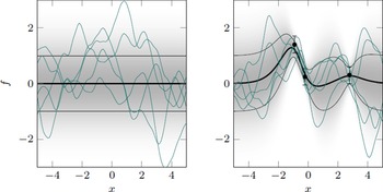
where we note again that $B_i(i)$ depends on $\pi$ and $\theta$ . The key idea of BO is to “learn” the landscape of the objective function $f(\pi, \theta)$ while searching for $\pi$ and $\theta$ that maximizes the objective function. BO first evaluates the function values $f(\pi, \theta)$ for some initial candidates of $\pi$ and $\theta$ and obtains a rough estimate for the landscape of $f(\pi, \theta)$ . In the next step, BO finds $\pi$ and $\theta$ such that the function value $f(\pi,\theta)$ and its uncertainty are both high, so as to balance the so-called exploitation-exploration trade-off. BO then evaluates $f(\pi, \theta)$ for these $\pi$ and $\theta$ and updates the estimate of the landscape of $f(\pi, \theta)$ . BO iterates this learning optimization procedure. Estimates of the maximizers $(\pi^*, \theta^*) = \arg \max f(\pi, \theta)$ are obtained after a sufficient number of iterations (Bull, Reference Bull2011).

The above procedure is called “Bayesian” because the learning of the objective function is done by a Bayesian nonparametric method (Rasmussen and Williams, Reference Rasmussen and Williams2006). The Bayesian method is used because it can yield both an estimate of the landscape and its uncertainties, which are crucial for the exploitation-exploration trade-off and for gaining the optimization efficiency. For implementation, we use the R package mlrMBO (Bischl et al., Reference Bischl, Richter, Bossek, Horn, Thomas and Lang2017) in our numerical analysis.

4.3. Simulation setting

We explain here how we approximate the expected utility in (4.3) by Monte Carlo simulations, which is necessary for applying BO. Moreover, we describe the problem setting for our numerical analysis in the next section. First of all, we set the number of working generations as $N = 40$ , the discounting factor in (4.3) as $\beta = 0.98$ , and the annual contribution as $c = 1$ .

4.3.1. Financial market

We consider three settings for the financial market that represent different market risks, to investigate when IRS in the IRS-DC model works most effectively. The market price of risk, a.k.a the Sharpe ratio, is defined by:

(4.4) \begin{equation} \lambda\;:\!=\;\frac{\mu-r}{\sigma}\end{equation}

where $\mu$ and $\sigma$ are the rate and volatility of the stock, respectively, and r is the rate of the risk-free asset; see Section 2.1.2. The Sharpe ratio quantifies the performance of a risky project in relation to a risk-free investment. It is one of the most frequently used performance measures, and we use it to describe different financial markets in our experiments. Typically, a Sharpe ratio above 0.5 in the long run indicates great investment performance and is difficult to achieve, while a Sharpe ratio between $0.1$ and $0.3$ is often considered reasonable and can be achieved more easily (e.g., Sharpe Reference Sharpe1998). Table 1 shows the Sharpe ratios for different financial markets estimated from historical dataFootnote 4. It shows that high values of the Sharpe ratio are around 0.3, and low values can be below $0.05$ .

Table 1.

Sharpe ratios of different financial markets estimated by empirical data for three financial markets from the United States, Germany, and China. We use the stock market index and the 10-year treasury bond as surrogates for risky and risk-free assets. We only have access to the data for the Chinese market after 2003. For each market, the Sharpe ratio is reported for two periods: from 1992 (or 2003 for China) to 2021, and from 2003 to 2010, the latter being a period around the financial crisis.

For the simulation, we consider the following three settings for the financial market, with different levels of the Sharpe ratio:

\begin{align*} & \mbox{Market 1:}\quad \lambda_1=\frac{\mu_1-r_1}{\sigma_1}=\frac{0.065-0.02}{0.15}=0.3; \\[5pt] & \mbox{Market 2:}\quad \lambda_2=\frac{\mu_2-r_2}{\sigma_2}=\frac{0.065-0.01}{0.25}=0.22; \\ & \mbox{Market 3:}\quad \lambda_3=\frac{\mu_3-r_3}{\sigma_3}=\frac{0.065-0.01}{0.5}=0.11.\end{align*}

We refer to Markets 1, 2, and 3 as M1, M2, and M3 for brevity, respectively. We call M1, M2, and M3 the markets with high, intermediate, and low Sharpe ratios, respectively. The calibrated values from the real world for the longer period (Table 1) justify the use of the chosen Sharpe ratios in our experiment.

4.3.3. Entry cohorts

The generations with indicators $i = 1, \dots, 40$ are those who participate in the IRS-DC plan at time $t = 0$ and are called entry cohorts. For $t < 0$ , that is, before participating in the IRS-DC plan, we assume that the entry cohorts participate in a pure DC plan that applies the optimal life cycle investment strategy, following Gollier (Reference Gollier2008). Namely, the pure DC plan invests a large amount into the stock when the participant is young and gradually reduces the amount invested in the stock as the participant approaches retirement. To be more precise, for a generation i where $i=1,\dots, 40$ , let $B_i(t)$ be the individual account of generation i and $Y_i(t)$ be the net present value at time t of all the future contributions of generation i; then the optimal fraction $\pi_i^{\textrm{ind}}(t)$ of generation i’s wealth to be invested in the stock is given by:

(4.5) \begin{equation} \pi_i^{\textrm{ind}}(t) \;:\!=\;\pi^c\frac{B_i(t)+Y_i(t)}{B_i(t)}.\end{equation}

See Merton (Reference Merton1971, Equation 71). Notice that $\pi^c$ is the so-called Merton constant defined as:

(4.6) \begin{equation} \pi^c\;:\!=\;\frac{\lambda}{\gamma\sigma},\end{equation}

where $\lambda$ is the Sharpe ratio in (4.4). Note that $Y_i(t)$ can be calculated straightforwardly here, as the interest rate risk is excluded.

For an individual with the CRRA utility function, the life cycle investment strategy (4.5) provides the highest expected utility (Merton, Reference Merton1971, Gollier, Reference Gollier2008). Hence, the life cycle investment strategy and its variants have been popular choices for pure DC plans (e.g., Booth and Yakoubov Reference Booth and Yakoubov2000; Haberman and Vigna Reference Haberman and Vigna2002). Note that, when an individual is young, the discounted future income $Y_i(t)$ is much higher than her current wealth in the account $B_i(t)$ , and thus $\pi^{\textrm{ind}}(t)$ in (4.5) is much larger than 1. Therefore, the life cycle investment strategy (4.5) implies a high-leverage (i.e., borrowing) strategy when the individual is youngFootnote 5 (see Figure 3).

Figure 3.

Realizations of the optimal life cycle investment strategy (4.5) for an individual who participates in the pure DC plan for her entire working period of 40 years. The left and right figures are for the Markets 1 and 3, respectively. Three values of the risk aversion $\gamma = 3, 5, 10$ are considered. The vertical axis represents (4.5) and the horizontal axis represents the time.

The life cycle investment strategy is also used in Section 5.5 to make a comparison between the IRS-DC and the optimal pure DC plans.

4.3.4. Euler–Maruyama approximation

For simulating the dynamics of the asset process (2.4), we use the Euler–Maruyama approximation. Given a finite time horizon $T > 0$ , we divide the interval [0, T] into n equal time intervals:

\begin{align*}[0,T]=[0,\Delta, 2\Delta,\cdots,n\Delta],\end{align*}

where we set the step size as $\Delta = 1 / 12$ , which corresponds to 1 month. Then we simulate the asset process as:

\begin{align*} &A(t+\Delta) = A(t) + (\pi(\mu-r)+r)\Delta + \pi\sigma\sqrt{\Delta}Z, \nonumber\\[5pt] &A(t)_+ = A(t) + 40c - B_t(t),\quad \text{if} \; t \in \mathbb{N} \cup \{0 \},\end{align*}

where Z is a standard normal random variable. The dynamics of the asset process in a pure DC plan is simulated in a similar way.

The step size $\Delta = 1/12$ implies that the indexation rate (2.11) is adjusted monthly according to the funding ratio. This monthly update is more frequent than the annual cash flows of the fund. This setting reflects the fact that the market values of individual accounts usually vary more frequently than cash flows in reality. The IRS-DC fund is assumed to be fully funded at $t=0$ implying that the initial value of the notional funding ratio is 1: $A(0)/L(0) = 1$ . (The influence of the initial funding ratio is examined in the numerical analysis in Section 5.2.)

5.1. Optimal investment strategy and adjustment parameter

As explained in Section 4.3, we consider nine different settings for the numerical analysis, resulting from three different values for the relative risk aversion ( $\gamma=3, 5, 10$ ) of the social planner and three different values for the Sharpe ratio ( $\lambda=0.3, 0.22, 0.11$ ) of the financial market. In each setting, we find the optimal investment strategy $\pi$ and the adjustment parameter $\theta$ by BO, as described in Section 4. We report the resulting optimal values of $\pi$ and $\theta$ in Table 2. For comparison, we also report the Merton constant (4.6) for each setting in Table 2, which will be used in the experiment in Section 5.5.

Table 2.

Optimal investment strategy $\pi^*$ and adjustment parameter $\theta^*$ obtained by Bayesian optimization for the nine different settings, resulting from the three different values of the Sharpe ratio $\lambda$ and the three different values of the risk aversion $\gamma$ . For comparison, the Merton constant is shown for each setting.

For each value of the Sharpe ratio $\lambda$ , the optimal $\pi^*$ and $\theta^*$ tend to decrease as the risk aversion $\gamma$ increases (with the exception of the case $\lambda = 0.3$ , where $\theta^*$ remains 1). Regarding the optimal investment strategy $\pi^*$ , this tendency can be anticipated by the same tendency in the Merton constant (4.6), which is inversely proportional to the risk aversion $\gamma$ . Regarding the optimal adjustment parameter $\theta^*$ , this tendency can be expected from the analysis in Section 3.3, where it is shown that a smaller adjustment parameter $\theta$ lowers the volatility of the retirement benefits; thus, a higher risk aversion $\gamma$ leads to smaller $\theta^*$ .

For each value of the risk aversion $\gamma$ , the optimal $\pi^*$ and $\theta^*$ tend to be smaller as the Sharpe ratio $\lambda$ becomes smaller (for the cases $\gamma = 3, 5$ and $\lambda = 0.22, 0.11$ , the adjustment parameter $\theta^*$ is comparably small). One can understand this tendency in a similar way as the discussion in the above paragraph, since the Sharpe ratio represents the market price of risk. Note that $\theta^*$ is extremely small for $\gamma = 10$ and $\lambda = 0.01$ , which implies the IRS-DC plan becomes similar to a DB plan, as discussed in Section 3.3; in this case, $\pi^*$ is also very small, meaning that the asset is mainly invested in the risk-free asset.

5.2. Funding ratio process

We next study the dynamics of the funding ratio $A(t)/L(t)$ , investigating the influences of the adjustment parameter $\theta$ and the initial funding ratio $A(0) / L(0)$ .

5.2.1. Influence of the adjustment parameter

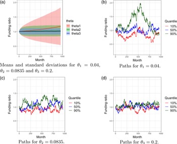
We first examine the influence of the adjustment parameter $\theta$ . We fix the investment strategy to $\pi = 0.131$ , which is optimal for Market 3 with $\gamma = 3$ (see Table 2). We consider three values for the adjustment parameter: $\theta_1 = 0.04$ , $\theta_2 = 0.0835$ , and $\theta_3 = 0.2$ , where $\theta_2$ is optimal for Market 3 with $\gamma = 3$ . For each value of the adjustment parameter, we simulate the IRS-DC fund 10,000 times in Market 3; the results are summarized in Figure 4.

Figure 4.

The influence of the adjustment parameter $\theta$ on the funding ratio process $A(t)/L(t)$ in Market 3. Panel (a) shows the mean and standard deviation of the funding ratio $A(t)/L(t)$ over 10,000 simulations as a function of time t, for $\pi = 0.131$ and each of three values of the adjustment parameter: $\theta_1 = 0.04$ , $\theta_2 = 0.0835$ , and $\theta_3 = 0.2$ . Panel (b) shows the paths of $A(t)/L(t)$ with $\theta_1 = 0.04$ corresponding to the top 10%, 50%, and 90% values of the utility of the social planner over the 10,000 simulations. Panels (c) and (d) show those with $\theta_2 = 0.0835$ and $\theta_3 = 0.2$ , respectively.

Figure 4(a) shows the mean and standard deviation of the funding ratio $A(t)/L(t)$ over the 10,000 simulations as a function of time t, for each of the three values of $\theta$ . The standard deviation is the smallest for $\theta_3 = 0.2$ and the largest for $\theta_1 = 0.04$ ; therefore, the larger the adjustment parameter, the smaller the standard deviation of the funding ratio. This observation validates our analysis in Section 3, which indicates that a larger adjustment parameter $\theta$ makes the funding ratio lower. Moreover, the mean of the funding ratio is close to 1 for $\theta_2 = 0.0835$ and $\theta_2 = 0.2$ , while the mean (and standard deviation) gradually increase for $\theta_3 =0.04$ . This observation is also consistent with the analysis in Section 3, which implies that a smaller adjustment parameter lets the funding ratio $A(t)/L(t)$ converge to 1 more slowly.

Figure 4(b), (c), and (d) show the paths of the funding ratio for three representative scenarios defined as follows. We pick up the three scenarios from the 10,000 simulations that correspond to the top 10%, 50%, and 90% values of the utilities of the social planner (see (4.2)) and plot the funding ratio processes in these scenarios; these three scenarios can be interpreted as representing “good,” “medium,” and “bad” realizations of the financial market. The discrepancy between the paths of the funding ratio in these scenarios reduces as $\theta$ increases. This implies that the funding ratio volatility decreases as $\theta$ increases and is consistent with our analysis in Section 3.

5.2.2. Influence of the initial funding ratio

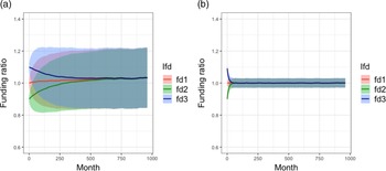
We next examine the influence of the initial funding ratio $A(0)/L(0)$ on the dynamics of the funding ratio $A(t)/L(t)$ . We consider three cases for the initial funding ratio: (1) $A(0)/L(0) = 0.9$ , (2) $A(0)/L(0) = 1$ , and (3) $A(0)/L(0) = 1.1$ . We simulate the IRS-DC fund 10,000 times for each case and calculate the mean and standard deviation of $A(t)/L(t)$ . Figure 5 shows the results for (a) Market 3 with $\pi = 0.131$ and $\theta = 0.0835$ , which are optimal for $\gamma = 3$ in Market 3, and for (b) Market 1 with $\pi = 0.267$ and $\theta = 1$ , optimal for $\gamma = 10$ in Market 1. Regardless of the initial funding ratio $A(0)/L(0)$ , the mean of the funding ratio $A(t)/L(t)$ converges to 1 as t increases. For Market 3, where the adjustment parameter $\theta$ is small, the mean of the funding ratio converges to 1 slowly; for Market 1, where the adjustment parameter is larger, the mean converges to 1 immediately. Therefore, these results suggest that the IRS-DC fund can self-stabilize the funding ratio to 1, and a larger adjustment parameter $\theta$ leads to a quicker stabilization; again, this is consistent with the analysis in Section 3.

Figure 5.

The influence of the initial funding ratio $A(0)/L(0)$ on the funding ratio process $A(t)/L(t)$ . Panel (a) shows the mean and standard deviation of $A(t)/L(t)$ in Market 3 over 10,000 simulations, for $\pi = 0.131$ and each of three settings of the initial funding ratio: $A(0)/L(0) = 1$ (red), $A(0)/L(0) = 0.9$ (green; underfunded), and $A(0)/L(0) = 1.1$ (blue; overfunded). Panel (b) shows those in Market 1 with $\pi = 0.267$ and $\theta = 1$ and the same three values of the initial funding ratio.

5.3. Dynamics of individual accounts

We next study the dynamics of individual accounts in the IRS-DC plan. As for the analysis in Section 3.4, to study the effects of IRS, each individual account in the IRS-DC plan is compared with the corresponding account in a pure DC plan that uses the same investment strategy $\pi^*$ in Table 2. (A pure DC plan using the optimal life cycle investment strategy is compared in Section 5.5.) Since IRS is absent, the dynamics of an individual account in the pure DC plan is given by the asset process yielding (3.12).

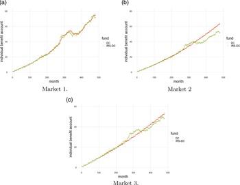
Figure 6 shows arbitrarily chosen paths of the individual accounts from the generation $i = 41$ in the IRS-DC and pure DC plans, for the three market settings and risk aversion $\gamma = 10$ . For Market 1, for which the adjustment parameter $\theta^*$ is large (see Table 2), the paths of the IRS-DC and DC accounts are similar. In contrast, for Markets 2 and 3, for which the adjustment parameter $\theta^*$ is smaller, the IRS-DC account accumulates more stably than the pure DC account. This observation is consistent with the discussions in Sections 2.1.5, 3.3, and 3.4 where it is argued that a smaller adjustment parameter $\theta$ reduces the volatility of an IRS-DC account as a result of IRS.

Figure 6.

Examples of paths of the IRS-DC and pure DC accounts for the generation $i =41$ in the three market settings with risk aversion $\gamma = 10$ .

We next quantify the effects of IRS on stabilizing the accumulation of an IRS-DC account. To this end, we calculate the increment-ratio-based roughness (IR roughness) (Bardet and Surgailis Reference Bardet and Surgailis2011), a measure of roughness/smoothness of a stochastic process, for each path of the IRS-DC and pure DC accounts. The IR roughness takes a value between 0 and 1, and a larger value indicates that the path is smoother; see Appendix C for details. Table 3 shows the average of the IR roughness over the 10,000 simulations for each of the IRS-DC and pure DC accounts from the generation $i= 41$ . For all the nine settings considered, the IRS-DC account has a larger IR roughness than the pure DC account, which implies that the IRS-DC account is smoother. Therefore, IRS makes the accumulation of the IRS-DC account more stable than the pure DC account (Recall that the only difference between the IRS-DC and DC plans here is the existence of IRS).

Table 3.

Average IR roughness over 10,000 simulations calculated for each of the IRS-DC and pure DC accounts, for the three market settings and the three levels of risk aversion.

5.4. Distribution of retirement benefits

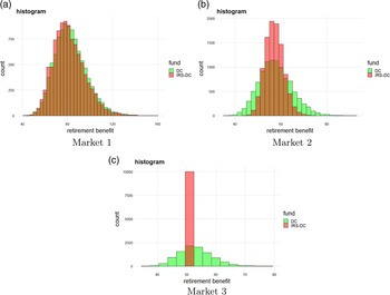
We next study how IRS affects the distribution of retirement benefits. Figure 7 shows the histograms of retirement benefits (from the 10,000 simulations) of the IRS-DC and pure DC accounts for the generation $i = 41$ , for the three market settings and risk aversion $\gamma = 10$ . (Results for $\gamma = 3, 5$ are shown in the online appendix.) For Market 1, for which the adjustment parameter $\theta^*$ of the IRS-DC plan is large, the histograms of the IRS-DC and pure DC retirement benefits are almost identical. On the other hand, for Markets 2 and 3, for which the adjustment parameter is smaller, the volatility of the IRS-DC benefits is smaller than the pure DC benefits. In particular, for Market 3, for which the adjustment parameter is close to 0, the volatility of the IRS-DC benefits is very small. These observations support the analysis in Sections 3.3 and 3.4 that a smaller adjustment parameter $\theta$ makes the retirement benefits less volatile by IRS. Moreover, our result is consistent with similar observations made by Bams et al. (Reference Bams, Schotman and Tyagi2016) and Donnelly (Reference Donnelly2017) that a collective DC scheme can reduce the volatility of retirement benefits.

Figure 7.

Histograms of the retirement benefits (obtained from the 10,000 simulations) of the IRS-DC and pure DC accounts for the generation $i = 41$ , for the three market settings and risk aversion $\gamma = 10$ . In each figure, the red and green histograms are those of the IRS-DC and pure DC benefits, respectively; the brown part shows the overlap between the two histograms.

5.5. Welfare of participants

Lastly, we study how IRS can improve the welfare of the IRS-DC plan participants in terms of their expected utilities. To this end, we make a comparison with a pure DC plan that uses the optimal life cycle investment strategy in (4.5), which yields the highest expected utility for an individual investor.

For simplicity, we assume that each participant in the IRS-DC plan has the same CRRA utility $U_\gamma$ in (4.1) as the social planner. Similarly, to make a comparison straightforward, we assume that each participant in the pure DC plan has the same CRRA utility. To measure the welfare, we calculate the certainty equivalent (CE) for each participant. That is, for an IRS-DC participant from the generation i with retirement benefit $B_i(i)$ , the CE is defined as the quantity $CE_{i}^{(\text{IRS-DC})} > 0$ satisfying

(5.1) \begin{equation}U_\gamma (CE_{i}^{(\text{IRS-DC})} ) = \mathbb{E}[U_\gamma (B_i(i))],\end{equation}

where we approximate the expectation in the right-hand side by the empirical average of 10,000 realizations of $B_i(i)$ . The CE of each participant in the pure DC plan is calculated similarly. Note that, since the utility function is strictly concave, the expected utility is monotonically increasing with respect to the CE; the higher the CE implies, the higher the expected utility. We calculate the CEs of the participants in the IRS-DC plan and the pure DC plans for the generations $i = 41, \dots, 80$ .

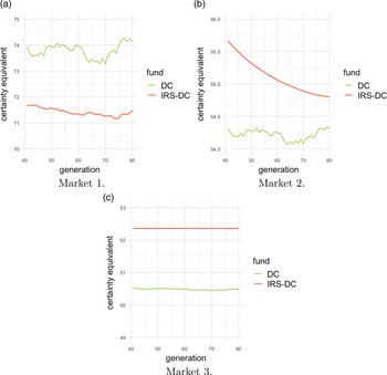
Figure 8 shows the CEs of the IRS-DC and pure DC participants for the generations $i = 41, \dots, 80$ , for the three market settings and risk aversion $\gamma = 10$ . (Results for $\gamma = 3, 5$ are shown in the online appendix.) For Market 1, where the Sharpe ratio is high, the pure DC participants obtain higher welfare than the IRS-DC participants. On the other hand, for Markets 2 and 3, where the Sharpe ratio is lower, the IRS-DC participants obtain higher welfare than the pure DC participants. This observation indicates that the IRS-DC plan can provide higher welfare than the optimal DC plan when the market is more volatile (in the sense of having a lower Share ratio). Therefore, IRS is expected to be particularly advantageous in protecting individual participants when the market is turbulent (e.g., when there is an economic shock).

Figure 8.

Certainty equivalents of the participants in the IRS-DC and pure DC plans for the generations $i = 41, \dots, 80$ , for the three market settings and risk aversion $\gamma = 10$ .

While it has been generally known in the literature that IRS is welfare-improving, there are a few key differences in our contribution. To explain this, we make a comparison with closely related works. Gollier (Reference Gollier2008) shows that IRS is welfare-improving over the optimal life cycle investment strategy, but his analysis is based on the assumption that the pension fund can perform borrowing for investment (i.e., the investment strategy $\pi$ can be larger 1); this assumption is not realistic for pension funds in reality. Moreover, his second-best strategy assumes the existence of a “shareholder” that helps finance the pension fund. Our result above shows that IRS can be welfare-improving even when borrowing is prohibited for the pension fund (i.e., $0 < \pi < 1 $ ) and without a shareholder.

Cui et al., (Reference Cui, De Jong and Ponds2011) show that a hybrid pension plan with IRS can provide higher welfare than a pure DC plan with an “optimal” investment strategy. However, their “optimal” individual investment strategy is not allowed to perform borrowing, and therefore it is less optimal than the optimal life cycle strategy (4.5), which performs borrowing. Moreover, Cui et al. (Reference Cui, De Jong and Ponds2011) optimize the parameters of the pension fund so as to maximize the expected utility of one specific entry cohort, not all the generations; they then compare this entry cohort’s welfare with a pure DC plan participant’s welfare. This way of optimizing the pension system is not appropriate as it ignores the other generations’ welfare. On the other hand, we show that the IRS-DC plan, which optimizes for all the generations’ utilities as in (4.3), can improve the welfare over the optimal life cycle investment strategy, when the market is volatile.

Bams et al. (Reference Bams, Schotman and Tyagi2016) consider a similar pension model as ours, but they do not show that their model can provide higher welfare than individual DC plans. Similarly, Donnelly (Reference Donnelly2017) considers a related collective DC plan but does not compare it with individual DC plans. Chen et al. (Reference Chen, Beetsma, Ponds and Romp2016) study a three-pillar model in which the second pillar is a collective DC, DB, or hybrid pension plan and make a comparison with the corresponding three-pillar model with the second pillar being an individual DC plan. While they show that the former yields higher welfare than the latter, they assume that the both plans use the same investment strategy, with the fraction invested in the stock being $\pi = 0.5$ ; therefore, their individual DC plan is not optimal. Different from these previous works, we make a comparison with the optimal life cycle investment strategy. By doing so, we show that the volatility of the financial market is a key factor that determines whether IRS is welfare-improving over the optimal life cycle investment strategy.