INTRODUCTION
Sorghum [Sorghum bicolor (L.) Moench] is a major source of forage for livestock in the semi-arid tropics. Improvement of forage sorghum cultivars for fodder yield is an important objective of the breeding programmes in this region. To ensure fodder security, there is a need to develop high-yielding cultivars widely adapted across target environments. Rainfall and temperature are unpredictable in the semi-arid tropics, resulting in inconsistent environmental conditions for crop growth and large genotype-by-environment interactions (GEI). Identification of high-yielding and stable genotypes across variable environments is often complicated by the frequent occurrence of GEI. To estimate and understand the complexity of GEI, plant breeders evaluate genotypes in multi-environment trials (MET) representing both favourable and unfavourable conditions, across target environments. Analysis of variance (ANOVA) of MET data provides estimates of genotype (G) and environment (E) main effects and GEI effects: G and GEI effects are mainly relevant to cultivar evaluation.
The genotype-by-environment interactions, defined as the variation in relative performance of genotypes in different environments (Cooper & Byth Reference Cooper, Byth, Cooper and Hammer1996), is a formidable challenge to plant breeders as it complicates testing and selection of superior genotypes, resulting in slow genetic progress (Romagosa & Fox Reference Romagosa, Fox, Hayward, Bosemark and Romagosa1993). A significant GEI may be either (i) a non-crossover type, where the ranking of genotypes remains constant across environments and the interaction is significant because of the changes in magnitude of the response, or (ii) a crossover type, where a significant change in rank occurs from one environment to another. Of these two types of GEI, crossover interactions are of more significance in plant breeding (Baker Reference Baker1988; Mohammadi & Amri Reference Mohammadi and Amri2013).
Besides identifying superior genotypes with broad adaptation, METs also provide an opportunity to detect differences among test sites, based on genotype response, which may provide a basis for regional sub-division into different mega-environments (MEs) (Yan et al. Reference Yan, Hunt, Sheng and Szlavnics2000). A ME is a group of growing areas that are similar in terms of genotype response and show a repeatable relative performance of crop genotypes across years (Gauch & Zobel Reference Gauch and Zobel1997; Yan & Rajcan Reference Yan and Rajcan2002: Yan & Tinker Reference Yan and Tinker2005). Several statistical methods have been proposed to subdivide environments or genotypes into homogeneous groups. ANOVA, principal component analysis and linear regression are traditionally applied to understand GEI in MET data (Zobel et al. Reference Zobel, Wright and Gauch1988). The advent and propagation of biplot methodology has addressed the complexity of GEI in a much simpler graphical manner (Gabriel Reference Gabriel1971). Among multivariate methods, the additive mean effects and multiplicative interaction (AMMI; Zobel et al. Reference Zobel, Wright and Gauch1988; Gauch Reference Gauch, Kang and Gauch1992) and genotype main effect plus GE interaction (GGE; Yan et al. Reference Yan, Hunt, Sheng and Szlavnics2000) biplot analyses are the methods most used for analysing GEI in MET data. Both methods have been developed and applied over recent years to analyse GEI and especially yield stability over environments in different crops. In recent literature, the utility of AMMI and GGE biplot analyses to visualize and interpret GEI data is being widely debated (Gauch Reference Gauch2006; Yan et al. Reference Yan, Kang, Ma, Woods and Cornelius2007; Gauch et al. Reference Gauch, Piepho and Annicchiarico2008; Yang et al. Reference Yang, Crossa, Cornelius and Burgueno2009). The ‘GGE biplot’ developed by Yan et al. (Reference Yan, Hunt, Sheng and Szlavnics2000) allows visual examination of the GEI pattern of the MET data. This method removes E and integrates G with GEI effects. Effectively, it detects the GEI pattern in the data and can identify ‘Which-won-where’, besides identifying different MEs (Yan et al. Reference Yan, Kang, Ma, Woods and Cornelius2007).
In the GGE biplot, a plot of genotype and environment generally is displayed by plotting the first two principal components (PC1 – primary effects, and PC2 – secondary effects) from the data. If the first two PCs cannot explain the complete variability in the data, other PCs may be brought in for interpretation. The GGE biplot can be used to (1) identify the best performing cultivar in a given environment, (2) identify the most suitable environment for a given cultivar, (3) compare any pair of cultivars across environments, (4) determine yield and stability of genotypes, (5) determine discriminating ability and representativeness of the environments and (6) most importantly, identify MEs (Malla et al. Reference Malla, Ibrahim, Little, Kalsbeck, Glover and Ren2010).
An important goal of any breeding programme is to identify the traits that contribute to higher yield. Fodder yield is a complex trait determined by several components that may affect the trait positively or negatively. Cultivar evaluation based on multiple traits is an important objective in plant breeding. It is important to examine the contribution of each of the component traits so that more focus may be given to those having greater influence on the target trait. The genotype–trait (GT) biplot, which is an application of the GGE biplot technique, is an excellent tool for visualizing genotype-by-trait data (Yan & Rajcan Reference Yan and Rajcan2002; Yan & Tinker Reference Yan and Tinker2005; Dehghani et al. Reference Dehghani, Omidi and Sabaghnia2008). These GT biplots summarize the genotype-by-trait matrix graphically (Yan & Rajcan, Reference Yan and Rajcan2002; Yan & Kang Reference Yan and Kang2003). Such biplots can be used to visualize correlations among traits, and identification of specific combinations is potentially useful for indirect selection (Yan & Tinker Reference Yan and Tinker2005). A GT biplot can also be used to visualize the performance of genotypes based on different traits which may enhance parental selection.
Analysis using GGE biplots has been carried out to characterize GEI in many crop species including soybean (Yan & Rajcan Reference Yan and Rajcan2002), rice (Samonte et al. Reference Samonte, Wilson, McClung and Medley2005), wheat (Kaya et al. Reference Kaya, Akcurra and Taner2006; Roozeboom et al. Reference Roozeboom, Schapugh, Tuinstra, Vanderlip and Milliken2008), barley (Dehghani et al. Reference Dehghani, Ebadi and Yousefi2006; Mohammadi et al. Reference Mohammadi, Aghaee, Haghparast, Pourdad, Rostaii, Ansari, Abdolahi and Amri2009), peanut (Putto et al. Reference Putto, Patanothai, Jogloy and Hoogenboom2008), lentil (Sabaghnia et al. Reference Sabaghnia, Dehghani and Sabaghpour2008), oats (Yan et al. Reference Yan, Fregeau-Reid, Pageau, Martin, Mitchell-Fetch, Etieenne, Rowsell, Scott, Price, De Hann, Cumminskey, Lajeunesse, Durand and Sparry2010, Martin et al. Reference Martin, Rubiales, Flores, Emeran, Shtaya, Sillero, Allagui and Prats2014), sorghum (Rao et al. Reference Rao, Reddy, Ratore, Reddy and Panwar2011; Rakshit et al. Reference Rakshit, Ganapathy, Gomashe, Rathore, Ghorade, Kumar, Ganesmurthy, Jain, Kamtar, Sachan, Ambekar, Ranwa, Kanawade, Balusamy, Kadam, Sarkar, Tonapi and Patil2012), linseed (Soto-Cerda et al. Reference Soto-Cerda, Westermeyer, Iniguez-Luy, Munoz, Montenegro and Cloutier2014), maize (Munawar et al. Reference Munawar, Hammad and Shahbaz2013) and others. Although there are many reports on the application of GE analysis to identify superior genotypes and/or test environments in many crops, such studies in forage sorghum are lacking. The GGE biplot technique was used to understand the stability of genotypes and also interpret complex GEI in grain sorghum (Rakshit et al. Reference Rakshit, Ganapathy, Gomashe, Rathore, Ghorade, Kumar, Ganesmurthy, Jain, Kamtar, Sachan, Ambekar, Ranwa, Kanawade, Balusamy, Kadam, Sarkar, Tonapi and Patil2012) and sweet sorghum (Rao et al. Reference Rao, Reddy, Ratore, Reddy and Panwar2011). The present paper reports on a study conducted to evaluate 16 forage sorghum genotypes across seven locations over 2 years (the rainy seasons of 2010 and 2011). The main objectives were (i) to interpret the complexity of GEI in forage sorghum using GGE biplot analysis; (ii) to identify high yielding stable genotypes that could be selected for the development of breeding populations; and (iii) to understand trait associations in forage sorghum using GGE biplot analysis.
MATERIALS AND METHODS
Plant material and testing locations
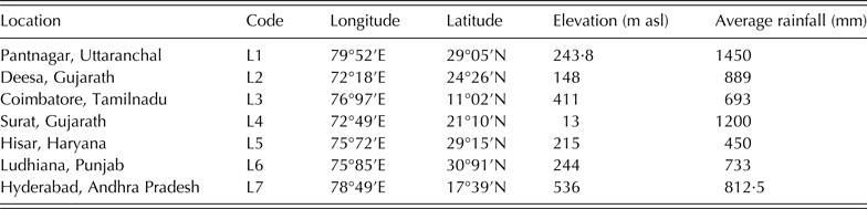
Sixteen forage sorghum genotypes were evaluated across seven locations during the rainy seasons of 2010 and 2011. Details of the testing locations are given in Table 1. The testing locations were distributed across six states of India, with two locations in Gujarat and one in each of the states Uttaranchal, Haryana, Punjab, Andhra Pradesh and Tamil Nadu.
Information on the study environments

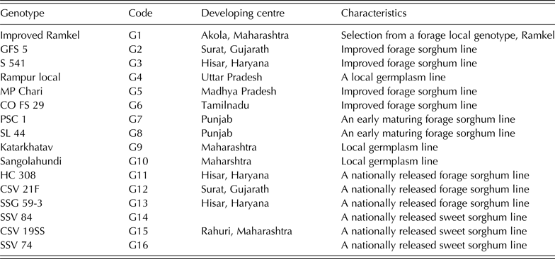
The material includes nine promising forage sorghum genotypes from different states of India, three nationally released forage sorghum varieties and three nationally released sweet sorghum varieties. The term ‘genotype’ is used in a loose sense to represent individual genotypes, lines, varieties or cultivars and details of these are given in Table 2. In both the years, the crops were sown during June–July depending on the onset of the monsoon season at each location. A randomized block design with three replicates was used at all locations. Each genotype was grown in two rows of 4 m length with 45 × 10 cm2 area. Standard crop management practices were followed across all locations. The data were recorded on morphological and yield traits at all locations during both the years of the field trials.
Information on the genotypes used in the study
Observations recorded
Observations were recorded on the following forage yield parameters: days to 50% flowering, plant height, early vigour, number of leaves per plant, leaf length, leaf breadth, stem girth, leaf-stem ratio and forage yield. Days to 50% flowering and forage yield were recorded on a plot basis, while other parameters were recorded on10 plants/plot taken at random. For forage yield measurement, all the plants in the plot were harvested at 50% flowering by cutting the stem manually at the base, and the entire above-ground plant material was weighed. The yields were recorded immediately after harvest to avoid moisture loss.
Data analysis
GGE biplot
A GGE biplot methodology consisting of two concepts, the biplot concept (Gabriel Reference Gabriel1971) and the GGE concept (Yan et al. Reference Yan, Hunt, Sheng and Szlavnics2000), was used to analyse the data. The statistical theory of GGE methodology has been explained in detail by Yan & Kang (Reference Yan and Kang2003). The multi-location trial (MLT) data was analysed as described by Rakshit et al. (Reference Rakshit, Ganapathy, Gomashe, Rathore, Ghorade, Kumar, Ganesmurthy, Jain, Kamtar, Sachan, Ambekar, Ranwa, Kanawade, Balusamy, Kadam, Sarkar, Tonapi and Patil2012) using the software GGE biplot ver. 6.3 (Yan Reference Yan2001). The MLT data was analysed without scaling (‘Scaling 0’ option) to generate a tester-centred (centring 2) GGE biplot, as suggested by Yan & Tinker (Reference Yan and Tinker2006). For genotype evaluation, genotype-focused singular value partitioning (SVP = 1) was employed using the ‘Mean v. stability’ option of the GGE biplot software, while for location evaluation, environment-focused SVP = 2 was employed (Yan Reference Yan2001) using the ‘Relation among testers’ option. The ‘Which-won-where’ option was used to identify which genotype was the winner in a given set of environments and to identify MEs. ANOVA, generated in the biplot software, was used for interpretation: it was conducted within each year across locations, and across both the years and locations.
Genotype-by-trait biplot
Genotype × trait biplots were generated in similar manner using the ‘Genotype-by-trait biplots’ option of GGE biplot software by combining data from all environments and using ‘Scaling 1’. Trait-focused SVP was used to determine phenotypic correlations among traits (Yan & Tinker Reference Yan and Tinker2005). Here, traits were considered as ‘tester’ and ‘Relation among testers’ was determined as described earlier.
RESULTS
Analysis of variance
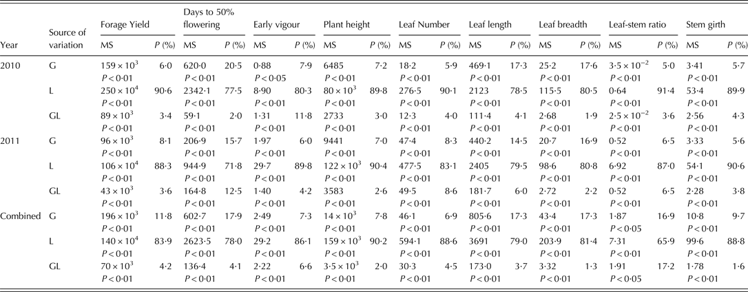
Relative magnitudes of the genotype (G), location (L) and genotype × location (GL) for all the traits studied are presented in Table 3. The ANOVA showed that genotype and location effects and GL effects were significant (P < 0·01) for all traits. Location was observed to be the most important source of variation for all traits, and its proportion ranged from 0·66 to 0·91 for different traits. For forage yield, the location accounted for 0·91 of the total variation in 2010 and 0·88 in 2011, and 0·84 in the combined analysis. Proportions of variation explained by GL were 0·03, 0·04 and 0·04 during 2010, 2011 and the combined analysis, respectively. Corresponding values for genotype were 0·06, 0·08 and 0·12 for forage yield.
Mean squares (MS) and per cent variation*(P) explained by genotype (G), location (L) and GL interaction for various traits
* Proportion of total variation (G + L + GL).
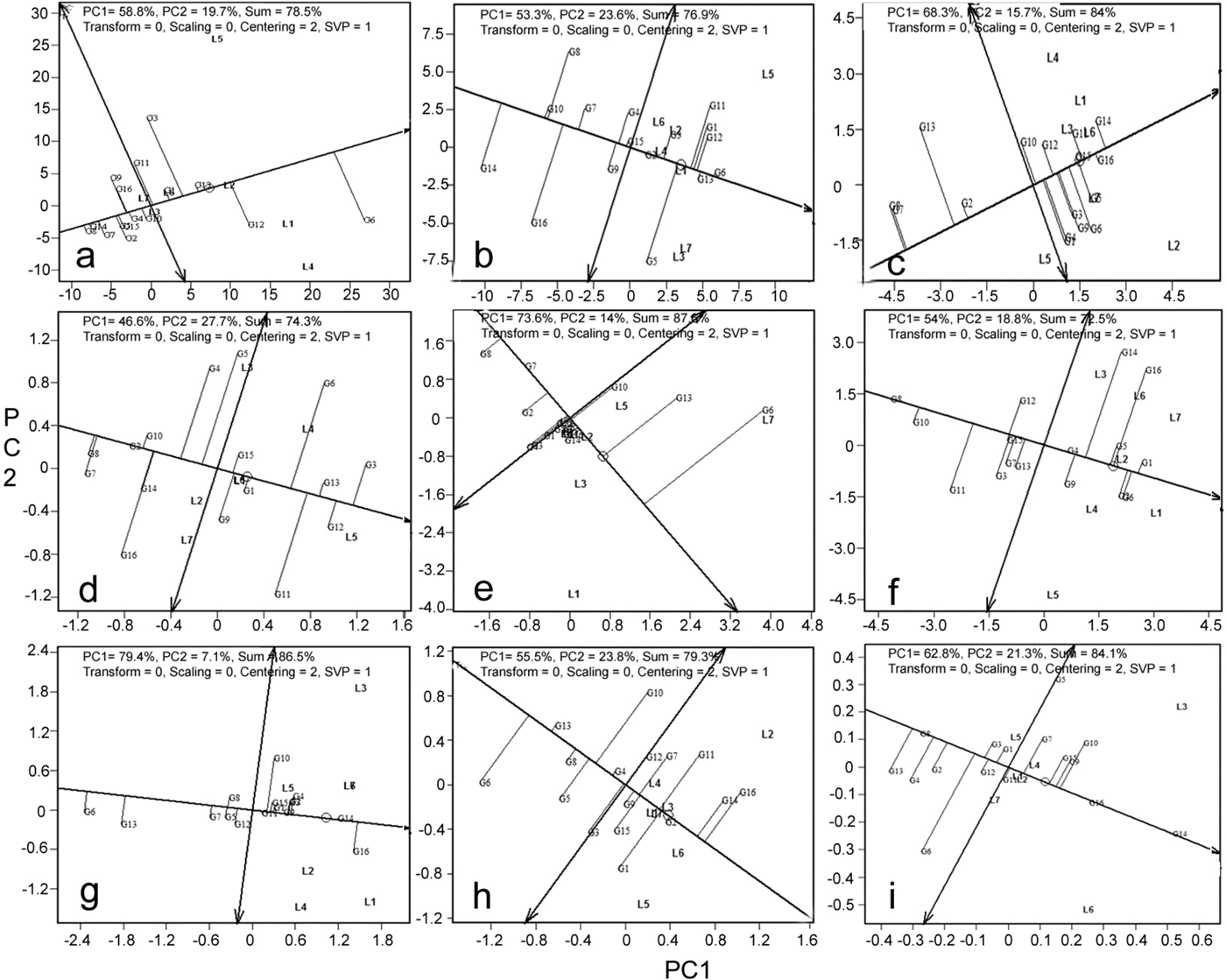
Mean performance and stability of genotypes across locations
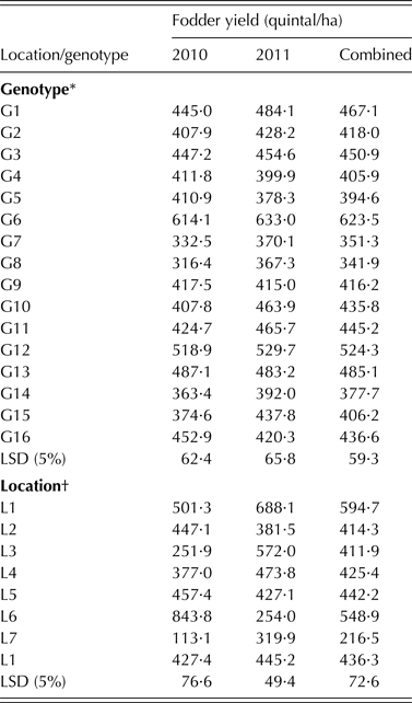
Performance of the entries based on the mean and stability is presented in Fig. 1, by the average environment coordination (AEC) method (Yan Reference Yan2001, Reference Yan2002). Since the within-year analysis showed more or less similar results, the results combined over years are presented. The environment-centred (centring = 2) genotype-metric (SVP = 1) biplots for each of the traits are presented in Figs 1(a)–(i). For forage yield, the first two PCs explained 79% of variation. In Fig. 1 the line with a single arrow head is the AEC abscissa, which passes through the biplot origin and points towards higher mean values. The perpendicular lines to the AEC passing through the biplot origin are referred to as AEC ordinates. These ordinates are depicted as double-arrowed lines in Fig. 1. The AEC abscissa ranks the genotypes for mean values. The genotype farthest from the origin would have either the highest (on the positive side of AEC abscissa) or lowest (on the negative side of AEC abscissa) mean yield. Accordingly, genotype G6 had the highest forage yield, being projected farthest from the origin on the positive side of the AEC abscissa, followed by G12 and G13. On the other hand, G8 showed the lowest forage yield, followed by G14. Comparison of biplot results with the mean yields of the genotypes (Table 4) showed that the biplot approximated the ranking of genotypes very well. Projection of the genotypes on the AEC ordinate approximated their stability. The higher the projection of the genotype on the AEC ordinate, the more unstable it is. It was observed that G6, followed by G3 and G12, were less stable for forage yield with higher projection from the AEC abscissa. On the contrary, G14, G8, G13, G1 and G4 were relatively stable as they were closer to the AEC abscissa. Of these, G13 had the highest forage yield after G6 and G12.
GGE biplots from the combined analysis of data from 16 forage sorghum genotypes (G1–G16) evaluated across seven locations (L1–L7) for the traits; (a) fodder yield, (b) plant height, (c) days to flower, (d) early vigour, (e) leaf number, (f) leaf length, (g) leaf breadth, (h) stem girth and (i) leaf-stem ratio (PC: principal component)
Year-wise and combined fodder yields of forage sorghum genotypes and locations under study over 2 years
* Genotype means are based on 7 location data over 2 years.
† Location means are based on 16 genotype data over 2 years.
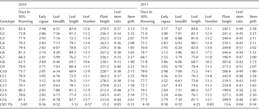
For forage sorghum, several other component traits are equally as important as forage yield. The mean and stability biplots for each of the yield component traits are presented in Figs 1(b)–(i). The analysis depicts desirable genotypes for each of these traits. The first two PCs explained 73–88% of the total variation in the data for different traits, which is sufficient to explain the complexity in the MLT data. For plant height, PC1 and PC2 explained 77% of the total variation and G6 was found to be the most desirable genotype, followed by G13, G12, G1 and G11. For days to 50% flowering, the biplot explained 84% of the variation. The genotypes G14, G16, G1, G15 and G5 fell under the late flowering category, while G8, G7, G13 and G2 were early flowering. The biplot of early vigour explained 74% of variation and G3, G12, G13, G11, G6 and G1 were promising for early vigour. Leaf numbers were higher in G6, G13 and G10, with the biplot accounting for 88% of variation. Longer leaves were observed in G1, G6, G2, G16, G5 and G14, and the biplot explained 73% of the variation. For leaf breadth, the biplot accounted for 87% of the variation and broad leaves were observed in G16 and G14. G14, G6 and G10 had high leaf-stem ratio, with the biplot explaining 84% of the variation. For stem girth, 79% of the variation was explained by the biplot, and G16, G14, G2 and G1 had larger girths. The measured values of these traits (Table 5) indicated very similar results in individual years, apart from minor changes in genotype ranking.
Year-wise data of other traits in forage sorghum genotypes under study over 2 years
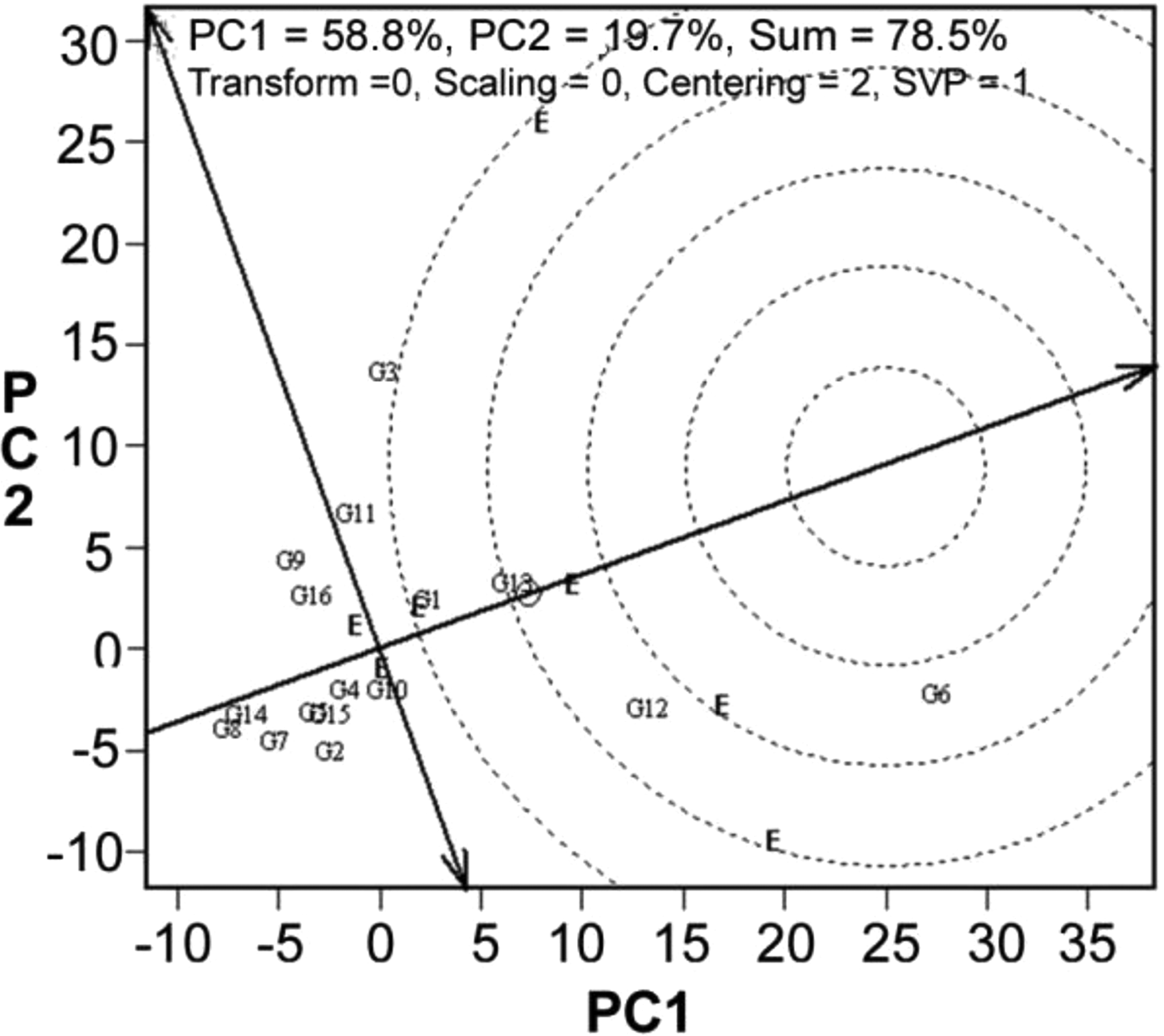
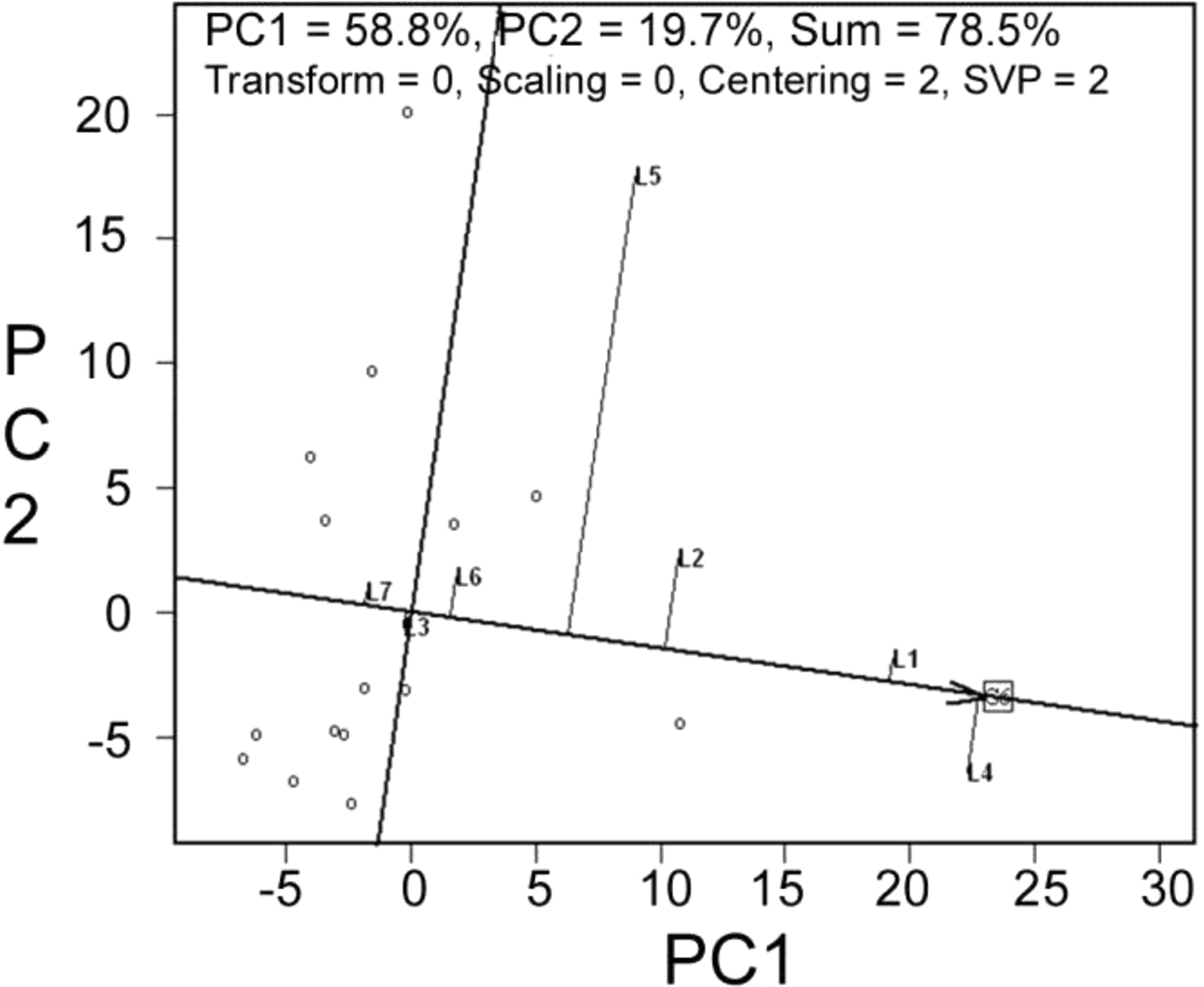
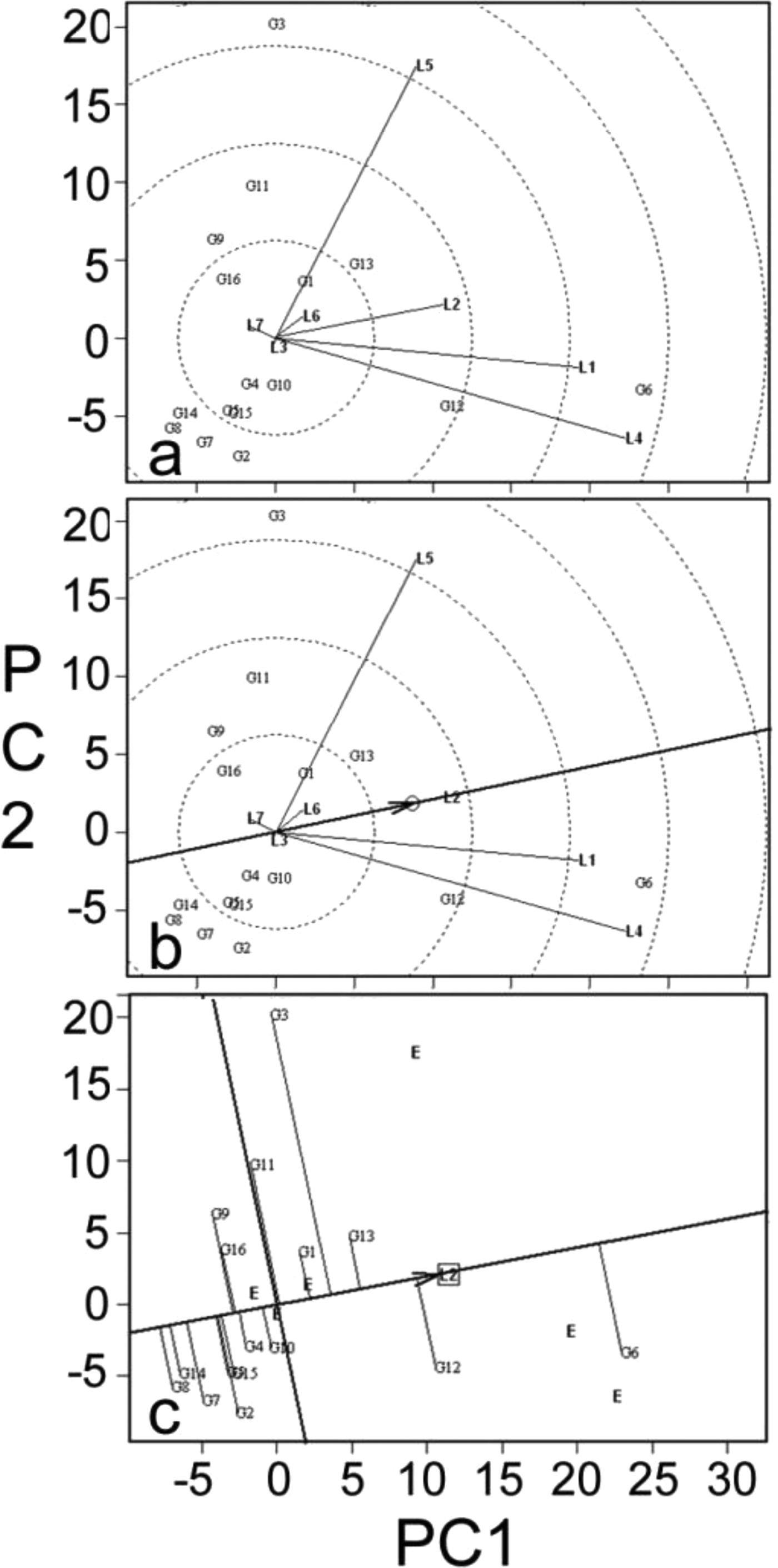
Since forage yield is the main trait under study, more focus was given to forage yield for subsequent analysis. Ranking of the genotypes for forage yield in terms of the ‘ideal genotype’ is presented in Fig. 2. An ‘ideal genotype’ is a high performer with high stability across environments (Yan & Tinker Reference Yan and Tinker2006). In the present study, G6, G12 and G13 were closer to the ideal genotype. These genotypes had high forage yield among all the genotypes tested (Table 4). G6, the highest yielder was used to study the specific adaptation by ranking the test environments based on the relative forage yield of this genotype in the given environment (Fig. 3). G6 had highest yields at L4 followed by L1, near average yield at L3 and L6, while below average yield at L7. In L2 and L5 it showed above average performance.
Ranking of 16 forage genotypes relative to an ideal genotype (the small circle on average environment coordinate, AEC)
Ranking of seven environments based on the performance of highest yielding genotype, G6
Environment evaluation in terms of forage yield
Multi-location trial data can also be used to understand about the test environments besides identifying superior genotypes (Cooper et al. Reference Cooper, Delacy, Basford, Cooper and Hammer1996; Yan et al. Reference Yan, Kang, Ma, Woods and Cornelius2007). Each test environment can be graphically evaluated in a GGE biplot for (1) its power to discriminate the genotypes, measured by its vector length in the biplot, and (2) its representativeness of other test environments, measured by its angle with the ‘average’ environment (Yan Reference Yan2001). Towards this goal, the relationships among test environments were studied by environment-metric SVP = 2 without scaling. The cosine of the angle between two environments reflects the correlation between them. An acute angle indicates a positive relationship between environments, while an obtuse angle is indicative of negative correlation and a right angle of no linear correlation (Yan & Tinker Reference Yan and Tinker2006). Combined analysis of the 16 genotypes across both the years for forage yield (Fig. 4(a)) showed that most locations were positively correlated. However, L7 had an obtuse angle with most other locations, suggesting a negative relationship. Location L5 was almost perpendicular to the rest of the locations, indicating no association (Fig. 4(a)).
GGE biplot showing (a) relation among the seven test locations; (b) ranking of locations based on discriminating ability and representativeness; and (c) Ranking of 16 forage genotypes based on their performance in the near ideal location, L2
Discriminating ability and representativeness of the test locations can be visualized by projection of the environments to the average environment axis (AEA) (Fig. 4(b)). The vector length of each location approximates its discriminating ability. Location L4, with the longest vector length, was found to be the most discriminating location, followed by L1, L5 and L2. Locations L6, L7 and L3 revealed no discriminating power, and therefore their correlation with other locations are not meaningful. Representativeness of a location can be visualized by projecting locations with respect to the AEC abscissa (Fig. 4(b)). The ‘average environment’ is represented by a small circle on the AEA in Fig. 4(b). Environments with smaller angles with the AEA are the most representative of the average test environments. Thus, L2 was closest to the average environment followed by L1 and others. An ‘ideal’ location as described by Yan (Reference Yan2001) is the one with the most discriminating and representative abilities. Test environments (locations) that are both discriminating and representative (e.g. L2, L1) are good test environments for selecting generally adaptable genotypes. While ranking the genotypes in the near average environment, L2 (Fig. 4(c)) showed that at L2, G6 yielded maximum followed by G12 and G13, while G8, G14, G7, G2, G15, G9, G16, G4 had lower than average fodder yield. G10 and G11 showed near average yield.
‘Which-won-where’ analysis and mega-environment identification
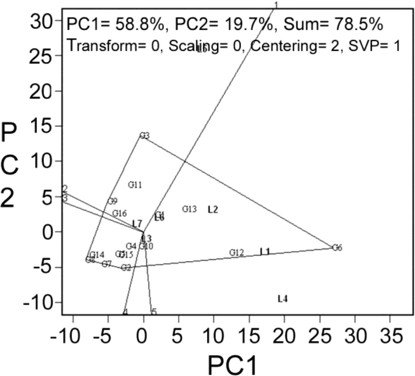
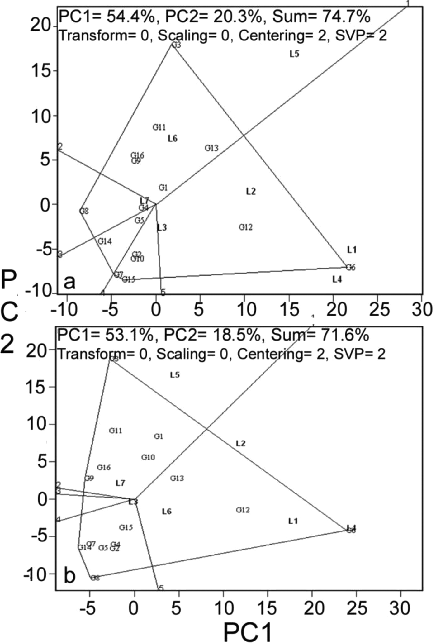
‘Which-won-where’ is the most interesting feature of GGE biplot, in which those genotypes farthest from the biplot origin are joined by straight lines forming a polygon, and perpendicular lines are drawn from the origin of the biplot to each side of the polygon. Thus, the biplot is separated into several sectors with one genotype at the vertex for each sector. ‘Which-won-where’ biplots for forage yield over 2 years is presented in Fig. 5 and for individual years in Fig. 6. The biplot indicated the existence of crossover GE and MEs. The polygon had four genotypes, viz. G6, G3, G14 and G2 at the vertices. The equality lines divided the biplot into three sectors, of which two retained all seven locations. Thus, the test locations may be partitioned into two MEs: one with L1, L2, L3, L4 and L6, with G6 as the best genotype. The second ME encompassed L5 and L7, with G3 as the best genotype. The genotype G6 performed best at L1, L2, L3 and L4 in both the years and in combined analysis over the years, while G3 was best in L5 and L7 (Fig. 6). In location L6, G6 was the best genotype in 2011 and in combined analysis, while G3 was best in 2010. No correlations were observed between the locations in one ME in terms of geographical location, rainfall pattern or altitude (Table 1).
GGE biplot indicating ‘Which-won-where’ analysis of the 16 forage genotypes for forage yield combined over years
GGE biplot indicating ‘Which-won-where’ analysis of the 16 forage sorghum genotypes during (a) 2010; (b) 2011
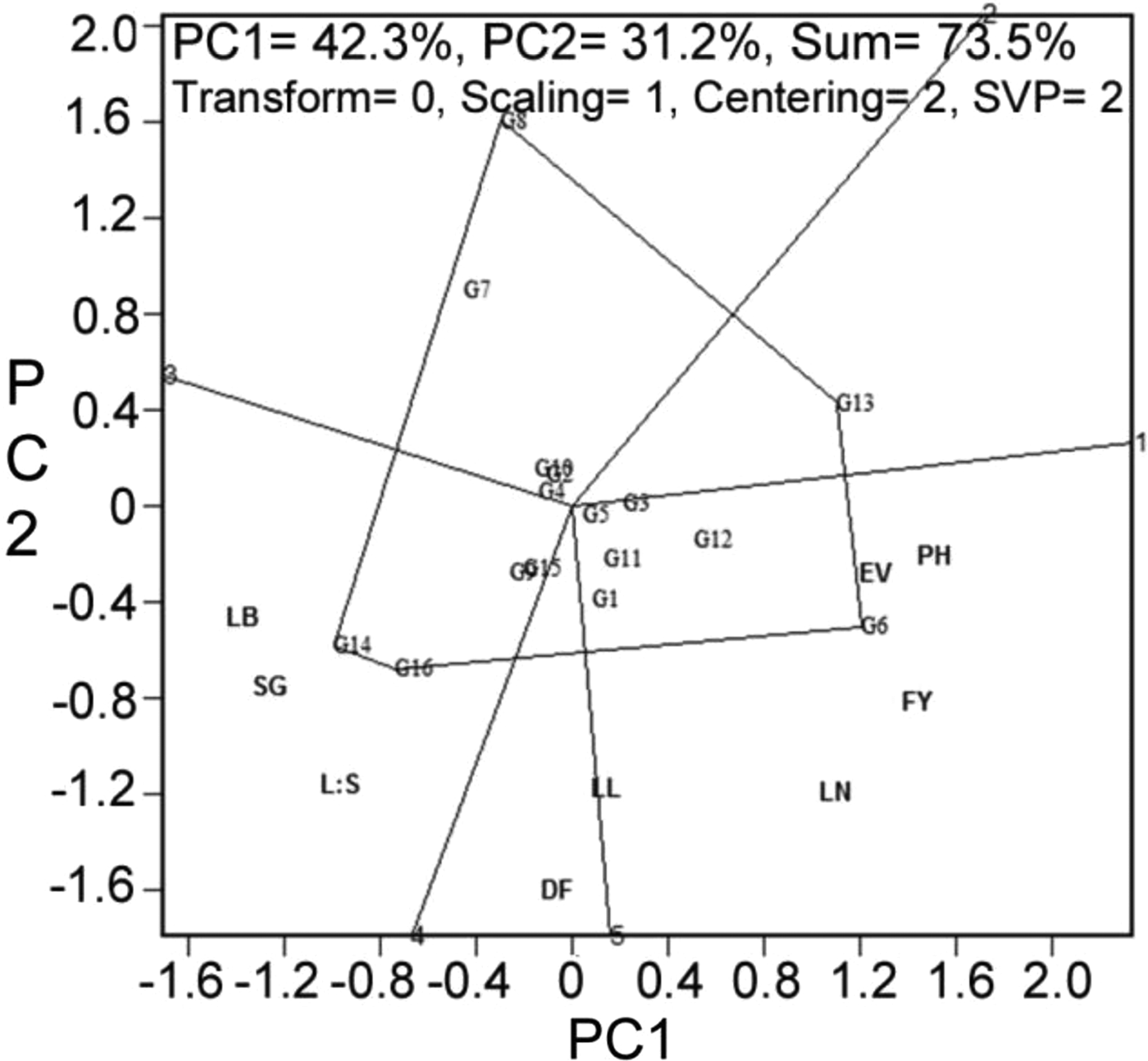
Trait associations through genotype-by-trait biplot
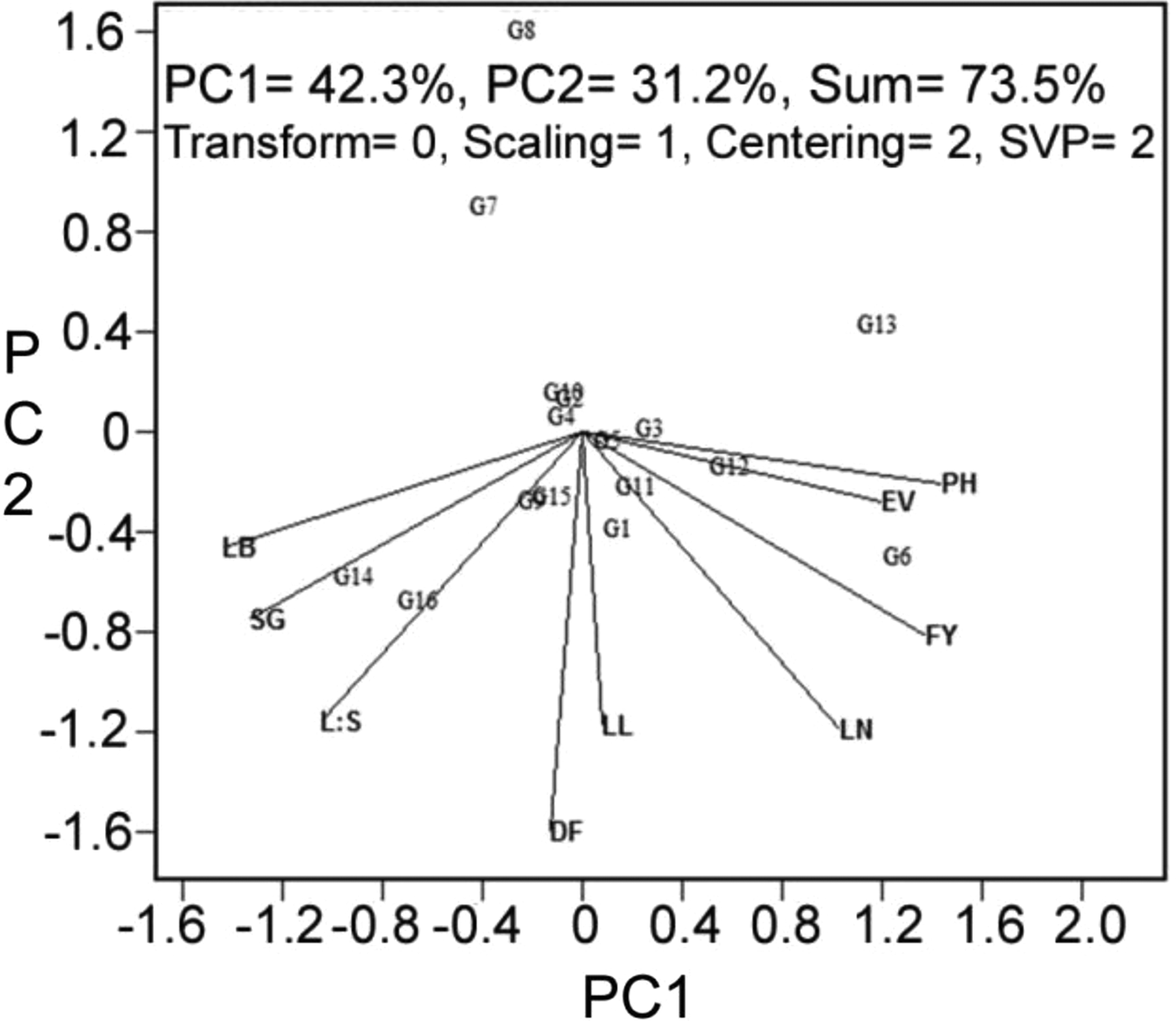
The G × T plot involving all nine traits under study facilitated visualization of the relationships among them (Fig. 7). The correlation coefficient between any two traits is approximated by the cosine of the angle between their vectors, as explained for the environments. The traits with shorter vectors indicate that there may be little variation among genotypes regarding the trait. The G × T biplot combined over 2 years explained 74% of the total variation in the data. Almost all the traits studied have contributed to the variation, as indicated by the vector lengths in Fig 7. The relationships among these traits are of more relevance in forage sorghum breeding. The most prominent relationships revealed by these biplots were: (i) strong positive association of forage yield with leaf number, early vigour and plant height, as indicated by the acute angles, (ii) a strong negative association of forage yield with leaf breadth and stem girth, as indicated by the large obtuse angles between their vectors. Forage yield and leaf-stem ratio were independent, since the angle between them is almost perpendicular.
GT biplot indicating inter-relationships among the measured traits from 16 forage sorghum genotypes
‘Which is best for what’ analysis helped to compare genotypes on the basis of multiple traits and to identify genotypes superior for particular trait(s) (Fig. 8). The biplot indicates that G6 was the best for forage yield, plant height, early vigour, leaf number and leaf length, while G16 and G14 were better for leaf breadth, stem girth and leaf-stem ratio.
Polygon view of GT biplot indicating which is best for what among the 16 forage sorghum genotypes
DISCUSSION
Successful forage sorghum cultivars need to be adapted to a range of environments, as yield stability is the most important aspect for popularity of any cultivar. Genotype × environment interaction is commonly observed as the differential ranking of genotypes across environments (Mohammadi & Amri Reference Mohammadi and Amri2013) and GEI for forage yield and quality in forage sorghum has been reported earlier (Aruna et al. Reference Aruna, Shrotria, Pahuja, Umakanth, Venkatesh Bhat, Vishala Devender and Patil2012). The GGE biplot is a tool to visualize the patterns of GEI in a graphical manner (Yan Reference Yan2001; Yan & Tinker Reference Yan and Tinker2006), and also helps in identifying relationships among traits and detecting the best genotypes for different traits. The complexity of the GEI in forage sorghum MLT data was investigated in the present study using GGE biplot analysis. Highly significant mean sum of squares observed in the present study indicated the sensitivity of the genotypes in terms of their responses to environments for fodder yield and other traits under study (Table 3). In the present study the first two PC explained >70% of the variability and G + GL explained >10% of variability for almost all traits. Thus, the biplots generated could be used effectively to interpret the variability in the MLT data. Location contributed 84–91% of the total variation in forage yield data, while contribution of genotype and their interaction with location was less. Gauch & Zobel (Reference Gauch and Zobel1997) reported that normally in MET data, environment accounts for 80% of the total variation. In grain sorghum MLT data, Rakshit et al. (Reference Rakshit, Ganapathy, Gomashe, Rathore, Ghorade, Kumar, Ganesmurthy, Jain, Kamtar, Sachan, Ambekar, Ranwa, Kanawade, Balusamy, Kadam, Sarkar, Tonapi and Patil2012) reported as much as 90% of the variation being explained by location. The present results were similar to these reports.
The GGE biplot provided information on genotype performance. The genotype COFS 29 (G6) was the highest yielding genotype followed by CSV 21F (G12) and SSG 59-3 (G13) (Fig. 1). However, COFS 29 and CSV 21F were less stable compared with other genotypes. Contrary to this, the most stable genotype, SSV 84 (G14) was among the poorest yielders. Earlier reports in grain sorghum also reported that the highest yielding genotypes are not necessarily the most stable (Rakshit et al. Reference Rakshit, Ganapathy, Gomashe, Rathore, Ghorade, Kumar, Ganesmurthy, Jain, Kamtar, Sachan, Ambekar, Ranwa, Kanawade, Balusamy, Kadam, Sarkar, Tonapi and Patil2012). One advantage of the graphical presentation of GEI is that genotypes closest to the ideal genotype can be identified conveniently (Yan & Tinker Reference Yan and Tinker2006). The ideal genotype (higher yielding and greater stability) is defined by having the longest vector length and zero GEI, and located at the centre of the concentric circles in Fig. 2. Genotypes located closer to the ‘ideal genotype’ are more desirable than others. Thus, COFS 29 (G6), CSV 21F (G12) and SSG 59–3 (G13) were closer to the ideal genotype. This would be difficult to conceive from a mean table alone. If genotype stability coupled with good forage yield is the focus of the breeding programme, then these genotypes should be selected. The GT polygon also indicated that genotypes COFS 29 (G6), SSG 59–3 (G13) and CSV 21F (G12) were promising for plant height, early vigour, leaf number along with fodder yield, while SSV 74 (G16) had broad leaves, larger stem girth and high leaf-stem ratio. Further, GT biplots indicated that leaf number, early vigour, plant height, leaf length and days to flower constitute one group of traits with positive effect on fodder yield (indicated by the acute angles among them). Leaf breadth and stem girth constitute another group. This suggested that the genotypes COFS 29, CSV 21F and SSG 59–3, which had a good combination of traits related to forage yield, could be used in breeding programmes focussed on yield improvement. The genotypes Improved Ramkel (G1), SSV 84 (G14) and SSV 74 (G16) could be good sources of genetic variation for improvement of leaf traits such as leaf length, leaf breadth and leaf: stem ratio.
The highest yielding genotype, COFS 29 (G6), performed best at Surat (L4) and Pantnagar (L1), with above average yields at Deesa (L2) and Hisar (L5), near average yields at Coimbatore (L3) and Ludhiana (L6), and less than average yield at Hyderabad (L7). The relationship between the testing environments was graphically presented using biplots where the angles between the vectors represented the type of correlation. The presence of wide obtuse angles between Hisar (L5) and Hyderabad (L7) and the other test environments suggested existence of negative correlation or strong crossover GEI for forage yield (Yan & Tinker Reference Yan and Tinker2006). This indicated that genotypes performing better in one environment would perform poorly in another environment. At the same time, closer relationships among other locations are indicative of non-existence of crossover GEI, suggesting that ranking of genotypes does not change from location to location. The present study clearly indicated that except for Hyderabad (L7) and Hisar (L5), all testing locations were closely related and most locations were close to the average environment. A mixture of crossover and non-crossover types of GEI in MET data is of very common occurrence (Kaya et al. Reference Kaya, Akcurra and Taner2006; Fan et al. Reference Fan, Kang, Chen, Zhang, Tan and Xu2007; Sabaghnia et al. Reference Sabaghnia, Dehghani and Sabaghpour2008; Rao et al. Reference Rao, Reddy, Ratore, Reddy and Panwar2011: Rakshit et al. Reference Rakshit, Ganapathy, Gomashe, Rathore, Ghorade, Kumar, Ganesmurthy, Jain, Kamtar, Sachan, Ambekar, Ranwa, Kanawade, Balusamy, Kadam, Sarkar, Tonapi and Patil2012). This may be due to some genotypes being highly responsive to change in the growing environment, while others are stable. Response to environment is purely a combined property of gene combinations in a given genotype. Different factors such as cropping season, rainfall, temperature regime, relative humidity and light intensity may contribute to GEI (Saeed & Francis Reference Saeed and Francis1984; Dehghani et al. Reference Dehghani, Ebadi and Yousefi2006). Identification of appropriate breeding and testing location is crucial to successful plant breeding programmes. It is important that testing locations must represent the population of target environments for which cultivar development is conducted. In the present study, the locations Surat (L4), Pantnagar (L1), Hisar (L5) and Deesa (L2) were identified as locations that had better discriminating abilities than the other locations, with long vector lengths. Similarly, Deesa (L2) was the most representative location, followed by Pantnagar (L1) and Ludhiana (L6). The locations Deesa and Pantnagar with good discriminating ability and representativeness are the suitable locations to identify genotypes with general adaptation. On the other hand, Surat (L4) and Hisar (L5), being discriminating and non-representative, are useful for selecting specifically adapted genotypes. Selection of appropriate test locations reduces the cost of MLT and improves breeding efficiency (Yan & Holland Reference Yan and Holland2010).
The ‘Which-won-where’ biplot, which graphically addresses crossover GE, ME differentiation, specific adaptation, etc. (Gauch & Zobel Reference Gauch and Zobel1997; Yan et al. Reference Yan, Hunt, Sheng and Szlavnics2000; Yan & Tinker Reference Yan and Tinker2006; Putto et al. Reference Putto, Patanothai, Jogloy and Hoogenboom2008; Rao et al. Reference Rao, Reddy, Ratore, Reddy and Panwar2011; Rakshit et al. Reference Rakshit, Ganapathy, Gomashe, Rathore, Ghorade, Kumar, Ganesmurthy, Jain, Kamtar, Sachan, Ambekar, Ranwa, Kanawade, Balusamy, Kadam, Sarkar, Tonapi and Patil2012), is the succinct summary of the GEI pattern of a MLT data set. Based on this analysis, the testing locations were partitioned into two MEs. ME1 was represented by Pantnagar (L1), Deesa (L2), Coimbatore (L3), Surat (L4) and Ludhiana (L6) with COFS 29 (G6) as the best genotype. ME2 consisted of Hisar (L5) and Hyderabad (L7) with S 541 (G3) as the best genotype. Partitioning of the target environments into meaningful MEs and deploying different cultivars for different ME is the best way to exploit the positive GEI (Yan & Tinker Reference Yan and Tinker2005). Identification of two MEs has several implications for future forage sorghum breeding and cultivar evaluation. Firstly, different cultivars should be deployed for the two MEs to achieve optimal adaptation. Secondly, although crossover GEI was observed frequently within the MEs, it could not be exploited effectively due to its unpredictability. The unpredictable GEI introduces uncertainty to cultivar performance and therefore should be avoided or minimized through breeding. This can be achieved through cultivar evaluation and selection focusing on genotype main effects or general adaptation within ME. Any measured yield at a given location in a given year is a mixture of year, location, and genotype main effects plus various interaction effects. Reliable selection for the genotype main effect requires removal of all other confounding variation, that is, the various year- and location-related effects (Yan et al. Reference Yan, Hunt, Sheng and Szlavnics2000). The only way to achieve this is to conduct multi-location trials over years. The finding that some testing locations were better than others for cultivar evaluation suggests that the uninformative locations may be dropped for evaluation of the genotypes without compromising the precision of evaluation. However, this ME pattern needs to be verified through multi-year and multi-environment trials, as conducted in wheat (Yan et al. Reference Yan, Hunt, Sheng and Szlavnics2000) and peanut (Casanoves et al. Reference Casanoves, Macchiavelli and Balzarini2005; Putto et al. Reference Putto, Patanothai, Jogloy and Hoogenboom2008). In the given situation smaller zonation of testing locations and focusing breeding efforts in a location-specific manner holds more importance.
In the present study, it is demonstrated that the use of two types of biplots, namely, the GGE biplot and GT biplot, facilitates understanding and exploration of GEI. The magnitude of genotype effects and GEI for fodder yield of 16 forage sorghum genotypes tested across seven locations over 2 years were much smaller than that of environment main effect. The genotypes exhibited both crossover and non-crossover types of GEI. Evidence of two MEs in the GGE biplot implies that different cultivars should be selected and deployed for the two MEs. The GT biplot can be used to aid genotype selection on the basis of multiple traits. The present study demonstrates that the GT biplot is an excellent tool for visualizing genotype-by-trait data. Firstly, it effectively reveals the interrelationships among the forage sorghum traits. Secondly, it provides a tool for visual comparison among genotypes on the basis of multiple traits. Based on the trait relationships, selection for forage yield improvement could be through plant height, leaf number, early vigour and leaf length using correlated response to selection.
The authors wish to thank Dr IK Das, Principal Scientist, DSR, Hyderabad, India for his help in improving the quality of the figures.