


Introduction
Deformation of single ice crystals in response to stress is strongly anisotropic. Crystals shear easily along the slip systems in their basal planes, much like a deck of cards, while shear on other slip systems is almost two orders of magnitude harder (Reference Duval, Ashby and AndermanDuval and others, 1983). The bulk strain rate of a polycrystalline aggregate subjected to stress depends on the orientations of the individual crystals within it. An aggregate may behave isotropically if the crystals within it have random orientations; it will behave anisotropically if the crystals within it have non-random orientations. The deformation of anisotropic ice has been studied extensively both in theory (Reference JohnsonJohnson, 1977; Reference AlleyAlley, 1992; Reference AzumaAzuma, 1994; Reference AzumaAzuma and Goto-Azuma, 1996; Reference CastelnauCastelnau and others, 1996; Godert and Hutter, 1998) and in the laboratory (Reference DuvalDuval, 1981; Reference DuvalDuval and LeGac, 1982; Reference Shoji, Langway, Langway, Oeschger and DansgaardShoji and Langway, 1985; Reference Pimienta, Duval and LipenkovPimienta and others, 1988; Reference Budd and JackaBudd and Jacka, 1989; Reference CastelnauCastelnau and others, 1998). The effect of anisotropy on the flow of an ice aggregate is significant enough that it is critical to understand its effect on large-scale flow patterns of ice sheets (Reference Russell-Head and BuddRussell-Head and Budd, 1979; Reference PatersonPaterson, 1991; Reference Mangeney, Califano and HutterMangeney and others, 1997; Reference CastelnauCastelnau and others, 1998; Reference Thorsteinsson, Waddington, Taylor, Alley and Blankenship.Thorsteinsson and others, 1999).
As ice undergoes viscous deformation, the crystal c axes tend to rotate toward the axis of greatest compressive strain (e.g. Reference PatersonPaterson, 1994). Thus, ice in glaciers and ice sheets typically has a non-random crystal-orientation fabric (the statistical pattern of crystal orientations within the bulk) depending on the strain-rate history (e.g. Reference AlleyAlley, 1992).
Despite evidence that ice within an ice sheet typically has a non-random crystal fabric, most ice-sheet models treat ice as an isotropic material (e.g. Reference RaymondRaymond, 1983; Reference Marshall, Tarasov, Clarke and PeltierMarshall and others, 2000; Reference Hulbe and PayneHulbe and Payne, 2001) because, in most cases, deviations from the flow field predicted by isotropic models that are due to non-random crystal fabric are small when compared to the overall flow field. As we require models to reproduce finer details of ice-sheet behavior, the effects of crystal fabric become more important. The ability to include the effect of crystal fabric in an ice-sheet flow law is important, for example, near ice divides where stratigraphy in ice cores may be affected (e.g. Reference Alley, Gow, Meese, Fitzpatrick, Waddington and Bolzan.Alley and others, 1997; Reference Waddington, Bolzan and AlleyWaddington and others, 2001).
On the scale of entire ice sheets, the effects of nonrandom crystal fabric may be parameterized through scalar ‘enhancement factors’ in the isotropic ice-flow law known as Glen’s law (Reference NyeNye, 1953; Reference GlenGlen, 1958); however, in order to know when these approximations are appropriate, we need to understand the effects of crystal fabric on ice-sheet flow patterns. We approach this question by focusing on flow near an ice divide using a two-dimensional plane-strain flow model of an ideal ice sheet.
In terms of their flow behavior, divides are unique when compared to other regions of ice sheets. This uniqueness poses an interesting challenge for ice-dynamics modeling because the shallow-ice approximation, which assumes that longitudinal stresses are negligible, is not valid near a divide. Yet, accurate models of flow near ice divides contribute significantly to interpretation of ice-core and borehole measurements, surface-motion measurements and observations of internal structure detected with ice-penetrating radar.
In the divide region of an ice sheet, the lowest deviatoric stresses are found near the bed and within one ice thickness of the divide (Reference RaymondRaymond, 1983). Because of the non-linearity of Glen’s law, the ice there has a significantly higher effective viscosity than the surrounding ice. The flow is impeded through this region of hard ice, altering flow trajectories and producing a special divide-flow pattern (Reference RaymondRaymond, 1983). Under the divide, older ice is closer to the surface than on the flanks, causing the isochrones to form an arch. This feature, which is often called a ‘Raymond bump’, is a characteristic signature of the non-linear flow law for ice. We can observe this layer arch in the internal structure shown by radio-echo sounding images (Reference Nereson, Raymond, Waddington and JacobelNereson and others, 1998a; Reference Vaughan, Corr, Doake and WaddingtonVaughan and others, 1999).
The divide layer arch (or lack thereof) has been used to infer past and present behavior of ice sheets (Reference Nereson, Raymond, Waddington and JacobelNereson and others, 1998a, b; Reference Nereson and WaddingtonNereson and Waddington, 2002). Since ice in an ice sheet typically exhibits a strong non-random crystal fabric, and ice flow is dependent on orientation of crystals relative to the applied stress, we expect that a non-random crystal fabric might affect the flow field. For example, when basal planes are aligned parallel to the plane of maximum shear stress, deformation may be enhanced by a factor of 8 or 10 relative to that for isotropic ice (Reference Budd and JackaBudd and Jacka, 1989; Reference AzumaAzuma, 1994; Reference AzumaAzuma and Goto-Azuma, 1996; Reference Castelnau, Duval, Lebensohn and CanovaCastelnau and others, 1996; Reference ThorsteinssonThorsteinsson, 2002). Characterizing the flow pattern resulting from a non-linear flow law that also includes the effects of crystal fabric will improve predictions by ice-sheet flow models and interpretations of the divide signature.
As a first step, Reference Mangeney, Califano and CastelnauMangeney and others (1996) modeled the flow of anisotropic ice near an isothermal divide in plane strain using a linear stress–strain-rate relationship for ice. We take the next step by combining an analytical description of deformation of a polycrystal with a vertically oriented crystal fabric together with a non-linear constitutive relation for bulk flow of ice. The analytical description is a linear version of the flow law derived by Reference ThorsteinssonThorsteinsson (2001). The benefit of this analytical description is its ability to capture the impact of crystal fabric on deformation near a divide, yet it is simple to implement in ice-sheet models.
An Anisotropic Constitutive Law for Ice
Empirically, an isotropic ice-crystal aggregate behaves as a power-law fluid (Reference NyeNye, 1953; Reference GlenGlen, 1955). The standard flow law most often used in ice-flow models is

where  and τij
are the strain-rate and deviatoric stress tensors, respectively, τ
eff is the effective shear stress (second invariant of the deviatoric stress tensor), n is the stress exponent (usually set equal to 3 for ice) and A
0 is the ‘softness parameter’. Strain rate is a function of temperature according to an Arrhenius relationship, where Q is the thermal activation energy for creep, R is the gas constant and T is temperature. The coefficient E is called the ‘enhancement factor’. In this form, all properties of the ice are lumped into the three scalars E, A and n. This form for the flow law is limiting for two primary reasons. First, ice deformation results from a combination of microscale mechanisms with different stress exponents (e.g. Reference AlleyAlley, 1992; Reference LangdonLangdon, 1996; Reference Goldsby and KohlstedtGoldsby and Kohlstedt, 2001; Reference Pettit and WaddingtonPettit and Waddington, 2003). Second, polycrystalline ice in an ice sheet can be strongly anisotropic; near a divide, the strain pattern (vertical compression combined with bed-parallel shear) drives the development of a vertically oriented crystal fabric (Reference AlleyAlley, 1992). When ice has a nonrandom crystal fabric, the components of the strain-rate tensor are not proportional to the corresponding components of the stress tensor; thus, except for cases in which a single component dominates the stress tensor, a scalar softness parameter or enhancement factor is ineffective at accounting for crystal fabric.
Several authors have presented anisotropic flow laws for ice (e.g. Reference AzumaAzuma, 1994; Reference CastelnauCastelnau and others, 1996; Godert and Hutter, 1998; Reference Gagliardini and MeyssonnierGagliardini and Meyssonnier, 1999; Reference ThorsteinssonThorsteinsson, 2001, 2002). Their approaches differ primarily in how they relate the stress applied to the ice aggregate to the local deformation rate of a crystal within the aggregate. At one end of the spectrum, the strain is assumed to be the same for all crystals; this is called the ‘homogeneous-strain assumption’ or the ‘Taylor–Bishop–Hill model’ (Reference TaylorTaylor, 1938; Reference Bishop and HillBishop and Hill, 1951). In this case, crystals that are favorably oriented for deformation (under the given state of stress) deform easily and shift the stress burden onto neighboring, unfavorably oriented, crystals. At the other end of the spectrum of anisotropic flow laws, the applied stress is the same for all crystals; this is called the ‘homogeneous-stress assumption’, based on the ‘Sachs model’ (Reference SachsSachs, 1928). Each crystal deforms at a rate dependent on its orientation, and grain boundaries migrate to ensure that no gaps develop between grains.
The real distribution of stress probably lies somewhere in between. The homogeneous-stress assumption requires all five slip systems to be active, because the deformation of an individual crystal is defined by the large-scale strain, which does not take into account the possibility that a crystal may be poorly oriented for slip on the basal plane. Because of this, the homogeneous-stress assumption may better describe the real deformation in ice, since each crystal deforms on its basal (easy) slip systems, and grain shape changes through grain-boundary processes (Reference ThorsteinssonThorsteinsson, 2000).
In this paper, we present results from two models for deformation of ice with a non-random crystal fabric. First we use the analytical model developed by Reference ThorsteinssonThorsteinsson (2001) (we will refer to this as ‘T2001’), which calculates the deformation of polycrystalline aggregates under combined stress environments. Second, we use a new model that is a restricted form of Reference ThorsteinssonThorsteinsson (2001) (we will refer to this as ‘ModT2001’), using a linear flow law for deformation within each crystal, which allows it to be incorporated in an ice-sheet flow model in a way that is computationally efficient.
T2001 uses the same basic assumptions as Godert and Hutter (1998) and Reference Gagliardini and MeyssonnierGagliardini and Meyssonnier (1999): it is based on the homogeneous-stress assumption. The bulk deformation of the ice aggregate is an integrated deformation of all the crystals within the aggregate. The resolved shear stress (RSS) on the basal plane of each crystal is a function of the c-axis direction relative to the applied stress field. The RSS drives the deformation of the crystal. To build a flow law from this theory, Reference ThorsteinssonThorsteinsson (2001) used a distribution of crystal orientations within an aggregate to define the bulk deformation. The fabric near an ice divide typically has a cluster of c axes, oriented vertically. This type of fabric can be approximated by defining a ‘cone angle’, which is the half-apex angle of a cone within which all crystals are uniformly distributed. This definition of cone angle applies to ideal ice aggregates; for a real aggregate, which may not have a uniform distribution of c axes within a cone, an ‘effective’ cone angle is defined which yields the same strain rate in response to the same applied stress under the same assumptions as the ideal aggregate; in practice, the effective cone angle is estimated from thin-section statistics (Reference ThorsteinssonThorsteinsson, 2000).
T2001 is an analytical solution which describes the deformation rate of the aggregate for a given effective cone angle under combined stress states. ModT2001 is a version of this analytical solution which uses a linear flow law. Compared to other formulations (Reference AzumaAzuma, 1994; Reference Castelnau, Duval, Lebensohn and CanovaCastelnau and others, 1996), T2001 and ModT2001 generally predict smaller enhancements. For example, for a single-maximum fabric deformed in simple shear on the basal plane, T2001 predicts an enhancement of 4.375, compared to ~9 for other models. ModT2001 predicts an even smaller enhancement of 2.5. Because of these smaller predicted enhancements, T2001 and ModT2001 both underestimate the role of anisotropy. T2001 (and therefore also ModT2001) has two limitations; it does not predict the evolution of the fabric and it does not include interactions between neighboring crystals (Reference ThorsteinssonThorsteinsson, 2002).
In order to incorporate the ModT2001 model into an ice-sheet flow model while maintaining the bulk flow nonlinearity, we use a bulk effective viscosity, η eff, which is derived from Glen’s law:

where A 0 and E are the isotropic softness parameter and enhancement factor and we assume the stress exponent, n, equals 3. By assuming a linear ice rheology for ModT2001, the strain rate can be described as a function of vertically oriented cone angle, α, and the effective viscosity:

where coefficients a, b, c, d and e are given as functions of cone angle, α, in Equation (A6) in the Appendix.
For plane strain, the stress-balance and conservation-of-mass equations can be rewritten as partial differential equations (PDEs). (A more complete derivation of these equations is given in the Appendix):



where u and w are velocities in the x and z direction, respectively; p is the pressure, ρ is the density, and g is the acceleration due to gravity. Subscripts x and z indicate partial derivatives. This derivation assumes that the softness parameter, A 0, and variables a through e are spatially uniform; therefore, these PDEs apply to individual finite elements and are not descriptive of the overall flow field.
Measurements of Crystal Fabric
Ice-sheet fabric can be measured in two ways. In the laboratory, ice-core thin sections viewed through cross-polarizing filters provide statistics of crystal orientation for tens to a few hundred crystals (e.g. Reference GowGow and others, 1997; Reference Thorsteinsson, Kipfstuhl and MillerThorsteinsson and others, 1997). In the field, a borehole sonic log measures the speed of sound transmitted through ~7 m of ice (containing many thousands of crystals) (Reference Thorsteinsson, Waddington, Taylor, Alley and Blankenship.Thorsteinsson and others, 1999). Sound speed reflects the elastic anisotropy, which is related to fabric in a straightforward way. Reference ThorsteinssonThorsteinsson (2000) relates this sonic-velocity measurement to an effective cone angle, which is a convenient measure for vertically symmetric fabrics often found near ice divides. Ice-core fabric data from thin sections can also be represented as an effective cone angle to compare with the sonic log. Reference Thorsteinsson, Waddington, Taylor, Alley and Blankenship.Thorsteinsson (2000) compared cone angles from the Greenland Icecore Project (GRIP) core calculated from sonic-velocity measurements to those calculated from thin sections and concluded that for highly symmetric fabrics the sonic velocity is the most useful; it is accurate and has a high vertical spatial resolution. In this study, we took advantage of the sonic log measured at Siple Dome, West Antarctica, (personal communication from G. Lamorey, 1999) which was converted to cone angle as a function of depth using the method described by Reference ThorsteinssonThorsteinsson (2000).
A First Estimate
To get a first estimate of the pattern of flow resulting from fabric similar to that seen at ice divides, we calculate the instantaneous enhancement of the vertical strain rate at a given cone angle for divide (pure shear) and flank (pure shear with simple shear) sites using T2001. The T2001 model is limited to predicting the deformation of an aggregate of ~1000 crystals; therefore, we calculate the effect for each depth in the ice sheet, without the stress redistribution of a fully coupled model. We show a similar calculation for the ModT2001 for comparison.
Figure 1 shows T2001 results as enhancement of the vertical strain rate due to crystal fabric under combined pure-shear and simple-shear stress states. Given a vertical cone angle and a relative amount of shear stress, the contours show the enhancement of the vertical strain rate relative to the vertical strain rate for isotropic ice. (Enhancements for other strain-rate components show different patterns.) We focus on vertical strain rate because, in the divide region, the shape of its depth profile is sensitive to the form of the flow law. Also, the difference between the shape of the vertical-velocity profiles at the divide and on the flank determines the size of the arch in the isochrones (Reference Pettit and WaddingtonPettit and Waddington, 2003).
Enhancement in vertical strain rate due to anisotropy for combined simple and pure shear. The horizontal axis is the ratio of the magnitude of the simple shear stress, σ s, to pure shear, σ n, such that the far left region represents flow dominated by pure shear (similar to ice-divide flow) and the middle and right regions represent flow dominated by simple shear (similar to flank flow). On the vertical axis the cone angle varies from 0° (strongly anisotropic) to 90° (isotropic). The cone angle associated with the maximum enhancement varies as the relative amount of shear stress varies. (Adapted from Reference ThorsteinssonThorsteinsson (2001).)

In Figure 1, the vertical cone angle associated with maximum enhancement of vertical strain rate varies from approximately 60° to 35° as the relative amount of shear stress increases. This is an expression of the differing direction of the maximum applied compressive stress (vertical on the left edge of the graph, approaching 45° on the right edge). The lower left region of the figure, where cone angles are less than 40°, represents ice that is stiff in vertical compression relative to isotropic ice. (Similar calculations for horizontal shear show that ice with this fabric is soft when undergoing horizontal shear.) If the crystals have a broader distribution of c axes (e.g. spread over a cone larger than 45°) then the ice is soft when compressed vertically, because enough crystals have basal planes tilted nearly parallel to the plane of maximum shear stress to allow deformation of the bulk.
We estimate the effect of this enhancement (or reduction) in strain rates near an ice divide using a cone-angle profile based on sonic-velocity measurements in the borehole at Siple Dome (personal communication from G. Lamorey, 2003; data are available only for the lower 800 m of the 1000 m thickness). The vertical cone-angle profile at a site within ten ice thicknesses of a divide should have the same general character as the divide profile, since the strain history of ice in both regions is similar. Therefore, in Figure 2 we calculate the enhancement in vertical strain rate (the ratio of the vertical strain rate calculated for anisotropic ice to that for isotropic ice:  for the cone-angle profile at Siple Dome assuming two different stress fields: one similar to the divide site (pure shear: σ
s/σ
n = 0) and one similar to a flank site (dominated by simple shear: σ
s/σ
n = 5). For comparison, we also provide the results of a similar calculation using the ModT2001 model (Equation (3)). Because ModT2001 is based on a linear flow law, the flank and divide profiles are identical.
Enhancement due to anisotropy in vertical strain rate  at divide and flank sites using fabric measured by sonic-velocity log in the Siple Dome borehole (no data were collected for the upper ~200 m). Results from T2001 are shown as thick (divide) and thin (flank) lines. ModT2001 for both flank and divide is shown as the dotted line (calculated from Equation (3)). Note the reduced enhancement with the linear ModT2001 model.

Figure 2 shows that throughout most of the depth of the ice sheet the ice is stiffer in vertical compression at the divide than on the flank. This difference in effective viscosity is similar in character to the viscosity difference described by Reference RaymondRaymond (1983) that results from the non-linearity of the isotropic flow law. The Raymond viscosity difference produces an arch in the isochrones and affects the depth–age scale at an ice divide. Figure 2 suggests that a cone-angle profile that decreases with depth (the fabric strengthens) can produce an arch in the isochrones similar to the Raymond bump. Since this conclusion is not based on an ice-sheet model that solves the complete stress-balance equations, it is only an estimate of the effect of crystal fabric on the divide-flow pattern. A more realistic assessment of an anisotropy-induced arch in the isochrones requires a numerical flow model with a flow law that incorporates the effect of anisotropy. Such a model can capture the redistribution of stress caused by the interaction of stress and fabric. To study the effect suggested in Figure 2 for a full ice-sheet model, we use the ModT2001 model, with the nonlinearity incorporated in the bulk ice-sheet flow model through the effective viscosity. Because of the limitation of the anisotropic description within this model, our results are an underestimate of the effect of crystal fabric.
Finite-Element Ice-Flow Model
We model an idealized divide with a thermomechanically coupled finite-element model. The geometry and approach are similar to Reference RaymondRaymond (1983) and Reference Mangeney, Califano and CastelnauMangeney and others (1996). The assumptions of the model include:
-
1. The ice deforms in plane strain; thus, the model best represents a ridge ice divide, such as Siple Dome (Reference Nereson, Waddington, Raymond and JacobsonNereson and others, 1996) or Roosevelt Island (Reference Conway, Hall, Denton,., Gades and WaddingtonConway and others, 1999).
-
2. We solve the heat-transfer equation for temperature using the surface temperature and the geothermal gradient at the base as boundary conditions. Conduction, advection and strain heating are included in the thermal model.
-
3. The upper surface is stress-free.
-
4. The divide is a line of symmetry where ice is constrained to move only vertically.
-
5. The horizontal-velocity profile on the flank boundary (at 30 ice thicknesses from the divide) carries away the integrated mass balance from the divide to the boundary in order to satisfy mass conservation for a steady-state ice sheet. We do not impose a vertical velocity on this boundary. Because our boundary is more than 20 ice thicknesses from the divide, the results for the region within 10 ice thicknesses of the divide are insensitive to the details of the horizontal-velocity profile on the flank boundary (Reference RaymondRaymond, 1983; Reference Schøtt, Waddington and RaymondSchøtt and others, 1992). In practice, however, we begin with a laminar-flow profile at the boundary, but as velocities within the ice sheet are calculated, we update the shape of the horizontal-velocity profile at the boundary to account for the unique rheological properties of the anisotropic ice and the non-uniform temperature field. We do this by maintaining constant ice flux out of the boundary, while applying a horizontal-velocity shape function calculated by the model at a distance of ten ice thicknesses from the divide.
-
6. The flow law with anisotropy is incorporated through a two-step calculation. First, an effective viscosity (η eff) is calculated for each element (see Equation (2)), where τ eff is determined from the effective strain rate,
 resulting from the previous iteration of the model This effective viscosity is substituted into Equations (4–6), which are solved for the new velocity gradients within each element given the cone angle, α. This process is repeated for a specified number of iterations (typically ten) to achieve convergence, which is defined through a maximum difference between velocity solutions in successive iterations. This two-step process allows us to combine the non-linear bulk flow of ice based on Glen’s law with a description of anisotropy based on a linear rheology.
-
7. In these models, we assume that the cone-angle profile is a function only of normalized depth, z/H(x).
-
8. The model solves the mass, momentum and energy conservation equations on a grid of nine-node quadratic elements for temperature, pressure and velocity fields.
 resulting from the previous iteration of the model
 This effective viscosity is substituted into
The physical characteristics of the model are chosen to approximate Siple Dome (Reference Nereson, Waddington, Raymond and JacobsonNereson and others, 1996): 1000 m thick, an accumulation rate of 0.12 m a−1, a surface temperature of −25°C and geothermal flux of 65 mWm−2. We used a 55 × 51 node mesh with elements concentrated in the divide region and near the bed. In the bulk flow law, Equation (1), we used values for A 0 based on those suggested by Reference PatersonPaterson (1994) according to the temperature of the ice calculated by the thermal model.
We initialized the surface profile using the shallow-ice approximation with isotropic fabric. The surface then evolved until it achieved a steady state in which ice flow was balanced by the prescribed accumulation rate. We consider our model to be in steady state when the root-mean-square change in the surface velocities within ten ice thicknesses of the divide does not exceed a specified tolerance (typically < 10−8 m a−1). The resulting solutions for different vertical profiles of crystal fabric, therefore, do not have the same ice thickness or surface profile; instead, they all have the same ice flux entering the surface and exiting the sides and all contain the same amount of ice within the model domain. For ease of comparison, we non-dimensionalized most of the results. Except where otherwise noted, horizontal and vertical velocities are expressed relative to the vertical velocity of ice at the surface at the divide (which for a steady-state divide is also the accumulation rate at the divide), and thicknesses are expressed relative to the ice thickness at the divide.
Model Results and Discussion
As discussed earlier, most measurements of crystal fabric near the centers of ice sheets show a similar pattern: isotropic ice near the surface and vertically aligned singlemaximum fabric at depth. The details of the cone-angle profile vary depending on the local history of climate, impurity content, temperature and strain rate. For this study, we choose four different piecewise-linear cone-angle profiles, shown in Figures 3a and d and 4a and d. Cone-angle profile A is based on a simple assumption of decreasing cone angle with depth. Cone-angle profile B adds the assumption of an increasing cone angle in deep ice due to recrystallization processes (this profile is loosely based on data from Greenland (personal communication from G. Lamorey, 2003)). Cone-angle profiles C and D are piecewise-linear profiles based on the measured sonic log from the Siple Dome borehole, shown as a dashed line in Figure 4a and d (personal communication from G. Lamorey, 2003). This paper presents results from eight different model runs using these four anisotropic profiles and an isotropic profile. The model runs are defined in Table 1.
The left column ((a) and (d)) shows cone-angle profiles A and B. The middle column ((b) and (e)) shows vertical-velocity profiles at the divide and flank; these are non-dimensionalized using the vertical velocity at the surface, w s (the accumulation rate for steady-state behavior). The right column ((c) and (f)) shows the horizontal-velocity profiles at 1,2 and 10 ice thicknesses from the divide, 1 H, 2H, 10H; these are non-dimensionalized using the vertical velocity of ice at the surface at the divide, w sdiv (the accumulation rate at the divide). Each plot shows three model results. Solid lines show velocities from anisotropic fabric with a non-linear flow law (AANL or BANL). Dashed lines show velocities from isotropic fabric with a non-linear flow law (INL). Dotted lines show velocities from isotropic fabric with a linear flow law (IL).

Plot of the model results for two cone-angle profiles based on the sonic log for Siple Dome. The plotting conventions are the same as in Figure 3. The dashed line in (a) and (d) is the measured cone-angle profile for Siple Dome (personal communication, Greg Lamorey, 2003).

Short-hand identification codes for our models

Figures 3b and e and 4b and e show the predicted vertical-velocity profiles at the divide and the flank for each cone-angle profile. Figures 3c and f and 4c and f show the horizontal-velocity profiles at 1, 2 and 10 ice thicknesses from the divide. For comparison, we include in each of these figures the solution for isotropic fabric with a non-linear flow law (INL, Equation (1) with n = 3) and isotropic fabric with a linear flow law (IL, Equation (1) with n = 1).
Cone-angle profiles A and C have consistently broader cone angles (>25°C) throughout the ice depth than profiles B and D. Their associated velocity profiles closely resemble those associated with isotropic fabric. Results from cone-angle profiles B and D, however, show significant differences in the shape of the vertical-velocity profiles when compared to the vertical-velocity profiles resulting from an isotropic cone-angle profile. These differences seem to be the result of the region of small cone angles present in both B and D. Cone-angle profile D, which is the closest approximation of the four to the fabric profile inferred from the measured sonic log from Siple Dome, includes a distinct band of tight vertical fabric. Duplicate logs demonstrate that this band is a real feature in the sonic-velocity log (personal communication from G. Lamorey, 2003). This band of fabric is bounded above by the Holocene/Wisconsin boundary near 700 m depth and bounded below by the onset of rapid recrystallization at just over 800 m depth. Cone-angle profile B, in contrast, has a broader band of tight fabric without strong gradients in cone angle.
The band of highly oriented crystals in the Siple Dome cone-angle profile D (Fig. 4d) concentrates the shear strain such that the band behaves like a false bed (Fig. 4f), reducing the stresses in the deeper ice. Figure 4f shows that the horizontal-velocity gradient across this shear zone strengthens with distance from the divide. The corresponding vertical-velocity profile shows small velocities in the deep ice, because most of the vertical strain occurs in the upper 70% (above the false bed).
In Figure 5, we highlight the differences between nonlinear and linear flow laws. The velocity profiles for cone-angle profile D are shown for both the non-linear (DANL) and the linear (DAL) solutions. For comparison, INL curves are also shown. The vertical velocity at the divide typically shows higher curvature for the non-linear case because of the decrease in deviatoric stress; this is the divide signature that produces the characteristic arch in the isochrones under a divide. In our model results (Fig. 5b), the DANL curve shows a higher curvature than the INL curve, while the DAL curve shows much less curvature than either non-linear model. This difference occurs because the effective viscosity for ice with linear rheology is not a function of the magnitude of the effective deviatoric stress, and, therefore, it is not a function of distance from the divide. With anisotropic fabric, the effective viscosity may be different for each component of the applied stress, but with a linear flow law these viscosities are not a function of the stress magnitude (or, therefore, the distance from the divide). As a result, the vertical-velocity profile at the divide for DAL closely resembles a flank vertical-velocity profile, rather than the non-linear divide profiles. At ten ice thicknesses from the divide (Fig. 5c, 10H), however, the DANL and the DAL curves are similar; both show the false-bed effect, although the velocity gradient is stronger in the DANL curve.
Velocity profiles for DANL, DAL and INL, to show the effect of the linear vs non-linear flow law. (a) Cone-angle profile (profile D). (b) Vertical-velocity profiles at divide and flank sites. (c) Horizontal-velocity profiles at 1, 2 and 10 ice thicknesses from the divide. In (b) and (c) solid lines show results from model DANL, dashed lines show results from model INL and dotted lines show results from DAL. Dashed line in (a) is measured cone angle for Siple Dome.

Because cone-angle profiles A and C show little change in shape of the velocity profiles when compared to that produced by the isotropic model, whereas cone-angle profiles B and D show significant change in shape, we conclude that an ice sheet needs cone angles smaller than 25° for the crystal fabric to have a significant effect on the divide-flow pattern (this is particularly evident when comparing the results from cone-angle profiles C and D, which are identical except for the tight band of fabric in the lower part of the ice sheet).
Although not all cone-angle profiles significantly change the divide-flow pattern, all the profiles show differences in their steady-state surface profiles between the anisotropic and isotropic models. Figure 6 shows these steady-state surface profiles, using both non-linear (Fig. 6a) and linear (Fig. 6b) flow laws. In this figure, the important difference between surface profiles is the shape, not the ice thickness. The steady-state ice thickness at the divide is a function of the ice-sheet span, which was not explicitly included in our model. If all modeled ice sheets had the same span, lower curvature at the divide would correlate with a thinner ice sheet and greater ice velocities because we maintain the same ice flux for all models and ice velocities scale as approximately the fourth power of ice thickness.
(a) Steady-state surface profiles resulting from models using each of the four cone-angle profiles with a non-linear flow law, identified with the code given in Table 1. Dashed line shows the surface predicted by the model with isotropic fabric and a non-linear flow law. (b) Results for isotropic fabric and two cone-angle profiles using a linear flow law. All models are plotted relative to the ice thickness at the divide for the isotropic model.

As shown in Figure 6, all anisotropic models have less curvature in the divide region than isotropic models. Further, the anisotropic models using a linear flow law (AAL and DAL, Fig. 6b) have less curvature than the non-linear models. If these models all had the same ice-sheet span, the anisotropic models would have significantly higher ice velocities. This result was first reached by Reference Mangeney, Califano and CastelnauMangeney and others (1996) for the case of a linear flow law. They examined the effect of a vertically symmetric crystal fabric on isothermal flow of a two-dimensional plane-strain ice divide with a linear flow law. Using a fabric that was isotropic near the surface and progressively more anisotropic with depth, they calculated the accumulation rate necessary to maintain the same steady-state ice-sheet thickness at the divide as the isotropic case. They found that 50% more accumulation is necessary to maintain the model ice-sheet thickness; this corresponds to larger horizontal and vertical velocities (by a factor of approximately 1.5), relative to the fully isotropic case. Shear was concentrated in the lower, more strongly anisotropic ice, causing the horizontal-velocity profile to have slightly higher curvature at depth and less curvature near the surface. Because the Mangeney model used a linear flow law, the shape of the velocity profiles did not vary with distance from the divide and no special divide-flow pattern was produced. Our results suggest similar increased velocities for anisotropic ice; additionally, we find that this effect is increased when a non-linear flow law is used.
Assuming that the cone-angle profiles and corresponding flow patterns in Figure 5 have existed for as long as the oldest ice in the ice sheet, we calculated the isochrone patterns produced from each model run. Selected results are shown in Figure 7. Model DANL, which most closely resembles Siple Dome, produced the largest isochrone arch. Model INL produced the next largest isochrone arch. Neither of the models using a linear flow law (DAL and IL) showed the development of an isochrone arch. The isochrone patterns produced by the other anisotropic models (AANL, BANL and CANL) all have arches with amplitudes intermediate between DANL and INL.
Isochrones in the divide region produced by anisotropic and isotropic fabric for an ideal ice sheet. The isochrones are plotted relative to the ice thickness on the flank (at ten ice thicknesses from the divide). The oldest isochrones are deep in the ice sheet, the youngest are near the surface. The largest isochrone arch is from the model with cone-angle profile D (Fig. 4d) and a non-linear flow law (DANL); the second largest is from the model with isotropic fabric and a non-linear flow law (INL). The flat isochrones are from the model using isotropic fabric and a linear flow law (IL), which is indistinguishable from the model using anisotropic fabric and a linear flow law (DAL).

To quantitatively compare the arches produced from all cone-angle profiles, we define an arch amplitude as the fractional height above a smooth curve that fits the isochrone along its flanks. In Figure 8 we plot this amplitude as a function of the relative height of the isochrone above the bed ten ice thicknesses from the divide. This graphical method for examining the isochrone arches was used by Reference Conway, Hall, Denton,., Gades and WaddingtonConway and others (1999) Reference Conway, Hall, Denton,., Gades and WaddingtonConway and others (1999) and Reference Nereson and WaddingtonNereson and Waddington (2002).
Amplitude of the isochrone arch as a function of depth. Labels identify results from each model. The results for the corresponding models with a linear flow law are shown with the group label ‘all linear models’. We express the arch amplitude (B) as the distance above a curve that best fits each isochrone along the flank of the ice sheet. It is plotted as a function of the relative height of the isochrone ten ice thicknesses from the divide.

As shown in the velocity profiles in Figures 3 and 4 and the arch amplitude profile in Figure 8, a linear flow law does not produce a significant arch in the isochrones, even when the ice has anisotropic fabric. As we discussed above, in order to produce the special divide-flow pattern, the effective viscosity for vertical strain must be a function of distance from the divide; this occurs when the viscosity is a function of the deviatoric stress. In other words, an isochrone arch is formed when the vertical strain rate is significantly different at the divide to that at the flank. Our results show that for a linear flow law and vertically oriented fabric, the anisotropic effective viscosities are minimally affected by the smaller deviatoric stress in the divide region. The subtle variations that do appear among the results from the linear-flow-law models in Figure 8 are due to the interaction between components of the anisotropic stress and strain-rate tensors (unlike the isotropic stress-strain-rate relationships, in which the strain-rate component is dependent only on the magnitude of the respective stress component, with anisotropy there is no one-to-one relationship between tensor components). If the cone-angle profile changes significantly with distance from the divide, it would be possible for a model with a linear flow law to produce an isochrone arch.
With the non-linear flow law, however, there is feedback between the deviatoric stress tensor and the effective viscosities. This feedback tends to redistribute the stresses within an ice sheet, such that regions of stiff ice support higher stresses (a form of ‘bridging’). These higher stresses then increase the strain rate; this decreases the stiffness, which, in turn, feeds back on the stress distribution. This feedback process does not exist for ice deforming with a linear rheology. When anisotropy is added to the non-linear constitutive relation, the crystal orientation affects this stress-redistribution feedback process; which, in turn, alters the divide-flow pattern.
Conclusions
From five cone-angle profiles (four anisotropic profiles and one isotropic profile), we find three primary effects on the ice-flow pattern near a divide. First, with the same accumulation rate, all models with a vertical preferred-orientation fabric reach steady state with an ice-sheet surface profile that has less curvature at the divide. If all models had the same ice-sheet span, the models that include a strong crystal fabric would be thinner at the divide and have higher velocities than models with isotropic fabric. To first order, this result does not depend on whether the flow law is linear or non-linear, although the details do depend on the non-linear flow law.
Second, when a non-linear flow law is used, anisotropic ice significantly affects the pattern of flow in the divide region when the effective cone angle decreases to less than ~25º. With the vertically oriented crystal fabric typically found near ice divides, a strong crystal fabric always increases the amplitude of the existing arch in the isochrones relative to the isotropic case. With a linear flow law, no arch exists in either the anisotropic or isotropic case.
Third, for the model with cone-angle profile most similar to Siple Dome (DANL), the crystal fabric tends to concentrate horizontal shearing within the band of small cone angles, producing a false-bed effect. Cone-angle profile B also shows shearing concentrated higher off the bed than in the isotropic case; because the gradients are not as strong, BANL does not show as strong a shear band as DANL.
The special divide-flow pattern first proposed by Reference RaymondRaymond (1983) results from the non-linearity of the flow law. The divide-flow pattern can also be altered by boundary conditions and ice-flow processes. In this paper, we focused on one ice-flow process: anisotropic deformation due to vertically oriented crystal fabric. Reference Pettit and WaddingtonPettit and Waddington (2003) focused on the other important ice-flow process: the shift to a linear deformation mechanism at low deviatoric stresses. They showed that when flow near a divide is described by a flow law combining a linear term and a nonlinear (Glen) term, the size of the isochrone arch is a function of the relative importance of the linear term: the isochrone arch is smaller when the linear term is larger. If we combine this two-term flow law with the anisotropic flow law presented here, the effect of the anisotropy is to modify the non-linear term almost exclusively. Therefore we expect that the pattern of flow at a divide that has low deviatoric stresses (low enough to be dominated by the linear term in the flow law) will not be significantly affected by crystal fabric, except for an overall decrease in thickness and increase in velocities. For divides that exhibit higher deviatoric stresses, strongly anisotropic ice will significantly affect the ice-flow pattern and, consequently, the interpretation of ice-core records, borehole logs, radar images and deformation measurements.
Acknowledgements
The work presented in this paper was supported by US National Science Foundation (NSF) grants OPP9615417 and OPP9815136, and an NSF Graduate Fellowship to E.C.P. We thank H. Conway and C.F. Raymond for ideas and comments. We thank the scientific editor S. Jones and two anonymous reviewers for helpful comments.
Appendix
T2001 and ModT2001 are based on the homogeneous-stress assumption, with deformation occurring as slip on the basal planes. Under this assumption, the applied stress is the same on all crystals within the aggregate. The deformation is determined by the crystal orientation through the resolved shear stress, which is the component of the applied stress acting on the three slip systems of the basal plane (the three a axes of the hexagonal ice crystal).
According to Reference ThorsteinssonThorsteinsson (2001), for a single crystal, the strain rate based on these assumptions is:

where (superscript c refers to a single crystal) and τ are the strain-rate and deviatoric stress tensors, respectively, β is a constant, A(T) is the softness parameter from Glen’s law for isotropic ice and n is the power-law exponent. R
(s) = (S + S
T
)/2 is the symmetric part of the Schmid tensor (S = b ⊗ n) for each slip system, s, where n is the normal to the basal plane and b is the Burgers vector. The resolved shear stress for a particular slip system, τ
(s), has the general form:
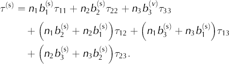
The bulk strain rate for the material results from the integral:

where F(θ, ϕ) is the c-axis-orientation distribution function (∫ ∫ F(θ, ϕ) dθ dϕ = 1), θ is the zenith angle measured from vertical and ϕ is the azimuth in the external reference frame.
From this point, we assume that n = 1 and that the F(θ, ϕ) function describes a single-maximum fabric with a vertical cone angle (α): F(θ, ϕ) = sinθ/[2π(1 − cosα)], for 0 ≤ θ ≤ α < π/2. We incorporate the non-linearity of the isotropic Glen flow law through iteration on η eff, which is the effective viscosity from Glen’s law:
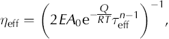
where β has been absorbed into the enhancement factor, E. At each step, η eff is calculated at the integration points of each element using the gradients of the velocities which were calculated in the previous step.
With these assumptions, Sachs’ law can be written:

where

In the limit of isotropy (lim α→90°), a = 2/3, b = c = −1/3 and d = e = 1.
Using the vector notation for the stress and strain tensors, Equation (A5) can be written as
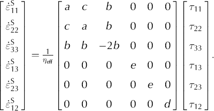
In order to invert the matrix in Equation (A7), we use the fact that the trace of the deviatoric stress tensor (τ 11 + τ 22 + τ 33) is zero and add a multiple (g) of that trace to the equation:
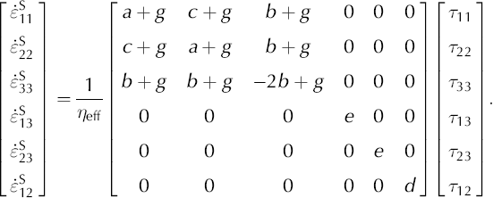
The inverse of this vertical-cone anisotropic constitutive equation, Equation (A8), is:
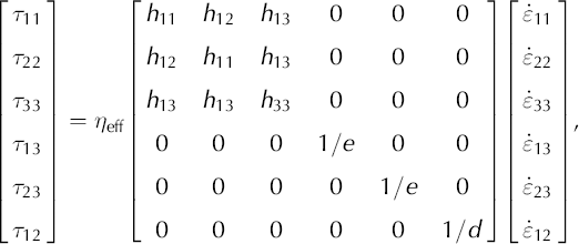
where
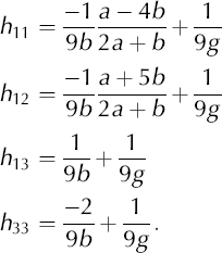
When we assume plane strain,  and Equation (A9) reduces to:
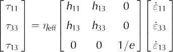
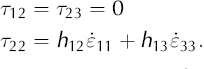
The transverse stress term, τ
22, is equal to zero for isotropic ice; however, for anisotropic ice this is not generally true, even under incompressibility,  The main implication of this is that τ
11 ≠ −τ
33. For an anisotropic material, non-zero deviatoric stresses may be required in all three directions to keep the flow confined within the plane. When we substitute velocity gradients for the strain rates, the constitutive Equations (A11) and (A12) become:
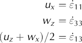
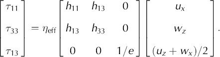
The final step in this derivation is to incorporate Equations (A13) and (A14) into the stress balance equations for the ice sheet. The stress balance equations are
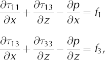
or


where f 1 and f 3 are source terms (in this application, we use f 1 = 0 and f 3 = ρg). These two equations plus incompressibility, ux+wz = 0, form the basis for our finite-element model. Incompressibility can, though, be used to simplify these equations to a form that is closer to the familiar form of Laplace’s equations,


For isotropic ice with a = 2/3, b = −1/3, e = 1, these two equations simplify to
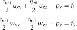
This derivation for Equations (A18) and (A19) assumes spatially uniform cone-angle functions (a through e) and a uniform η eff. This assumption applies to an individual element, not to the flow field as whole.



