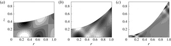
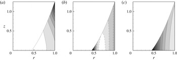
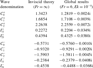
1. Introduction
When a cylindrical container, such as a glass or a pail, is partially filled with a liquid and put into rotation at a constant rate around its vertical axis, the free surface deforms as a consequence of centrifugal effects and eventually relaxes to a parabolic shape. This simple situation, which is now often encountered as an exercise in undergraduate fluid dynamics courses, was first discussed by Newton (Reference Newton1687), who described the motion as follows: ‘If a vessel, hung by a long cord, is so often turned about that the cord is strongly twisted, then filled with water, and held at rest together with the water; after, by the sudden action of another force, it is whirled about in the contrary way, and while the cord is untwisting itself, the vessel continues for some time this motion; the surface of the water will at first be plain, as before the vessel began to move; but the vessel by gradually communicating its motion to the water, will make it begin sensibly to revolve
 $[\cdots \,]$
till at last, performing its revolutions in the same times with the vessel, it becomes relatively at rest in it’ (Newton Reference Newton1687). After this description of the transient dynamics, which are now explained as a result of viscous stress originating from the walls and leading to a relaxation to solid body rotation and a parabolic surface, Newton put forward a philosophical argument intended as a proof of the existence of an absolute space: ‘This ascent of the water shows its endeavour to recede from the axis of its motion; and the true and absolute circular motion of the water, which is here directly contrary to the relative, discovers itself, and may be measured by this endeavour.’ In other words, an observer located in the same frame as the bucket, even if he perceives the water as perfectly still, could still infer that the bucket is in rotation by a simple observation of the curved surface.
Reconsidering the original argument of Newton from a modern point of view, one could argue that, even without noticing the concavity of the surface, an observer located in the frame of the bucket could convince himself that he is rotating with respect to an inertial frame by observing that small amplitude perturbations give rise to wave motions. Indeed, several kind of waves directly due to rotation or affected by it can be expected to occur in the present situation. At least three families of waves can be anticipated. First, for frequencies of the order of the rotation rate, one expects to encounter inertial waves which are directly due to the restoring effect of the Coriolis force (Greenspan Reference Greenspan1990). Second, at much lower frequencies, the radial variation of height of liquid plays a similar role to that of the zonal variation of the Coriolis parameter in planetary flows, so one can also expect the existence of Rossby waves. Finally, surface waves due to the restoring effect of gravity are also encountered, and one can expect to detect the effects of rotation on their characteristics.
Despite the academic interest linked to its historical significance, only a few studies have investigated the oscillation modes of the Newton bucket configuration, and most of them focussed on the sloshing modes without rotation (Henderson & Miles Reference Henderson and Miles1994; Bauer & Eidel Reference Bauer and Eidel1997; Martel, Nicolas & Vega Reference Martel, Nicolas and Vega1998; Ibrahim Reference Ibrahim2005), or restricted to either the weak rotation regime (Miles Reference Miles1964) or the fast rotation regime (Sun Reference Sun1960; Miles & Troesh Reference Miles and Troesh1961), where the free surface remains flat at leading order or forms a hollow cylindrical core, respectively. However, beyond its fundamental interest, there are several practical situations where it is desirable to possess a comprehensive description of the various wave solutions of the Newton bucket configuration. First, the fact that it gives rise to an almost perfect parabolic surface has been exploited in at least two applications. The first is in producing liquid mirrors, which has been achieved in large telescopes looking at the zenith by slowly rotating a circular tank filled with quicksilver or gallium (Borra Reference Borra1982). The second is linked to the production of contact lenses by the spin casting process, in which liquid polymer is injected into a spinning mold (Neefe Reference Neefe1983). In both these situations, it may be desirable to know the frequencies at which the free surface is more likely to vibrate, leading to potential disturbances of the desired shape. Second, a closely related situation, in which only the bottom plate is rotating while the lateral wall is held fixed, has been the object of a number of recent experiments (Vatistas Reference Vatistas1990; Jansson et al. Reference Jansson, Haspang, Jensen, Hersen and Bohr2006; Suzuki, Iima & Hayase Reference Suzuki, Iima and Hayase2006; Poncet & Chauve Reference Poncet and Chauve2007; Bergmann et al. Reference Bergmann, Tophøj, Homan, Hersen, Andersen and Bohr2011) because it gives rise to the onset of spectacular three-dimensional patterns, including rotating polygons, switching and sloshing. Recently, an explanation of such phenomena in terms of resonance between several kinds of waves has been proposed (Tophøj et al. Reference Tophøj, Mougel, Bohr and Fabre2013; Fabre & Mougel Reference Fabre and Mougel2014; Mougel, Fabre & Lacaze Reference Mougel, Fabre and Lacaze2014). The proposed mechanism requires some differential rotation, so it is not directly applicable to the Newton bucket configuration, for which all wave solutions are expected to be stable (namely, oscillating or weakly damped). However, experimental observations and a theoretical argument by Bergmann et al. (Reference Bergmann, Tophøj, Homan, Hersen, Andersen and Bohr2011) demonstrate that a substantial part of the flow, in the central region, is actually close to solid body rotation, so having at hand a catalogue of the wave solutions existing in this configuration is highly desirable. Also, it is worth pointing out that the new apparatus by Bach et al. (Reference Bach, Linnartz, Vested, Andersen and Bohr2014) is characterized by independent rotation between the cylinder wall and the bottom plate, and therefore allows one to switch between the two above-mentioned configurations, namely Newton’s bucket and the rotating bottom experiment.
The objective of this work is, thus, to provide an exhaustive and comprehensive classification of all the waves existing in the Newton bucket configuration, for a range of parameters ranging from zero rotation and a flat surface to strong rotation and highly deformed surfaces (with the possible appearance of a dry central core). For each family, we will detail the structure of the eigenmodes and the physical mechanisms behind it, and explore the effect of the parameters (the most important being the Froude number characterizing the ratio between rotation and gravity effects) on the frequency and damping rate. For this purpose, we will employ a combination of various approaches, including numerical solution of the global stability equations in the viscous case, a simpler approach valid in the shallow-water approximation which allows some analytical results, and a number of asymptotic approaches. The paper is organized as follows: in § 2 we describe the geometry and the parameters, present the general linear equations governing small-amplitude waves in the viscous case, and introduce the global stability method used to solve them. In § 3, we analyze the mathematical structure of the inviscid problem, first from the general equations, and second from the point of view of the shallow-water approximation. Section 4 is devoted to the exploration and classification of the wave solutions, relying mostly on the numerical solution of the global stability problem, with comparisons to approximate solutions of the inviscid problem whenever possible. Section 5 explores the effect of viscosity and boundary conditions on the waves, in particular by comparing the results with either no-stress or no-slip conditions along the walls. Section 6 briefly addresses the case where the cylinder is closed by a top wall, leading to different phenomena in the high-Froude-number limit. Finally, § 7 summarizes the results and lists a few open directions for future studies.
2. Problem setting: geometry, parameters, and governing equations
2.1. Geometry and parameters
In cylindrical coordinates
 $(r,{\it\theta},z)$
we consider a cylindrical container of radius
 $R$
partially filled with water and rotating around its vertical axis of symmetry at a constant rotation rate
 ${\it\Omega}$
with respect to an inertial frame. The gravity field is constant and vertical, with acceleration
 $g$
. The volume of fluid filling the cylinder is fixed and is
 ${\rm\pi}R^{2}H$
, where
 $H$
denotes the height of the flat free surface at rest. The first dimensionless parameter is thus purely geometrical, and corresponds to the aspect ratio
 $$\begin{eqnarray}a=\frac{H}{R}.\end{eqnarray}$$
In the general case we consider an incompressible, viscous liquid of density
 ${\it\rho}$
and kinematic viscosity
 ${\it\nu}$
. Surface tension is neglected. The physics of this problem is thus controlled by three main ingredients, namely rotation, gravity and viscosity. Taking the cylinder’s radius as a length scale, the three associated time scales respectively read
 $T_{{\it\Omega}}={\it\Omega}^{-1}$
,
 $T_{g}=\sqrt{R/g}$
and
 $T_{{\it\nu}}=R^{2}/{\it\nu}$
. Pertinent non-dimensional numbers can be constructed by comparison between these time scales. The most important one is obtained by comparing gravity and rotation, and yields the Froude number
 $$\begin{eqnarray}Fr=a^{-1/2}\frac{T_{g}}{T_{{\it\Omega}}}=\frac{{\it\Omega}R}{\sqrt{gH}}.\end{eqnarray}$$
Note that the aspect ratio
 $a$
has been conveniently incorporated into this definition. Under this form, the Froude number can also be interpreted as the ratio between the characteristic velocity of the fluid and the surface wave velocity in the shallow-water limit, so this choice will prove to be particularly convenient.
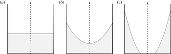
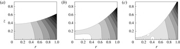
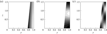
Typical free surface shapes: (a)
 $Fr=0$
, (b)
 $Fr<2$
, (c)
 $Fr>2$
.

The third important parameter needed in the analysis can be constructed by comparing the viscous time scale with the other effects. For instance, comparing rotation and viscosity leads to the Ekman number
 $$\begin{eqnarray}Ek=\frac{T_{{\it\Omega}}}{T_{{\it\nu}}}=\frac{{\it\nu}}{R^{2}{\it\Omega}}.\end{eqnarray}$$
At equilibrium, the whole volume of fluid rotates rigidly with the solid walls; the azimuthal velocity in the inertial frame thus corresponds to
 $V(r)={\it\Omega}r$
. Neglecting surface tension, the free surface shape is governed by the equilibrium between centrifugal force and gravity, which leads to the famous parabola. Two regimes should be considered for the equilibrium state (further called base flow) depending on whether the Froude number is below or above the critical value
 $Fr_{c}=2$
. If
 $Fr<2$
, the minimum water height remains positive and the water covers the entire bottom. This situation will be referred to as the wet case. On the other hand, when
 $Fr\geqslant 2$
the fluid does not entirely cover the container bottom (see figure 1). In other words, a circular dry region appears at the centre and this situation will thus be referred to as the dry case. The equation for the free surface is given, in each case, by
 $$\begin{eqnarray}\displaystyle \left.\begin{array}{@{}c@{}}\displaystyle \text{Wet case }(Fr<2):\quad h(r)=H+\frac{{\it\Omega}^{2}}{2g}\left(r^{2}-\frac{R^{2}}{2}\right)\equiv a\left[1+Fr^{2}\left(\frac{r^{2}}{2}-\frac{1}{4}\right)\right]\!,\\ \displaystyle \text{Dry case }(Fr>2):\quad h(r)=\frac{{\it\Omega}^{2}}{2g}\left(r^{2}-R^{2}\right)+\sqrt{\frac{{\it\Omega}^{2}HR^{2}}{g}}\equiv a\frac{Fr^{2}}{2}\left(r^{2}-{r_{c}}^{2}\right)\!.\end{array}\right\} & & \displaystyle\end{eqnarray}$$
In each case, the second expression given here is non-dimensional (with
 $R$
as a length scale), and
 $r_{c}$
is the non-dimensional radius of the dry region defined by
 $r_{c}=\sqrt{1-2/Fr}$
. The pressure distribution corresponding to this base state is given as
 $P_{0}(r,z)=P_{a}+{\it\rho}g(h(r)-z)$
, where
 $P_{a}$
is the pressure at the free surface.
Finally, it should be noted that the equilibrium state does not depend upon the viscosity of the fluid. Viscosity would only impact the rate at which the equilibrium is reached.
2.2. Global stability equations
We consider, in the following, small perturbations of the base flow defined previously. We thus expand velocity, pressure and fluid height as follows
 $$\begin{eqnarray}\displaystyle & \displaystyle [U,V,W,P]=[0,{\it\Omega}r,0,P_{0}(r,z)]+[u(r,z),v(r,z),w(r,z),{\it\rho}p(r,z)]\text{e}^{\text{i}m{\it\theta}-\text{i}{\it\omega}t},\quad & \displaystyle\end{eqnarray}$$
 $$\begin{eqnarray}\displaystyle & \displaystyle H(r)=h(r)+{\it\eta}(r)\text{e}^{\text{i}m{\it\theta}-\text{i}{\it\omega}t}. & \displaystyle\end{eqnarray}$$
 $m$
is the azimuthal wavenumber and
 ${\it\omega}$
is the complex frequency of the wave. Classically, we have
 ${\it\omega}={\it\omega}_{r}+\text{i}{\it\omega}_{i}$
, where
 ${\it\omega}_{r}$
is the oscillation rate and
 ${\it\omega}_{i}<0$
is the damping rate. Note that the oscillation rate in the rotating frame corresponds to
 ${\it\omega}_{r}-m{\it\Omega}$
.
The linearised equations for the perturbations then read
 $$\begin{eqnarray}\displaystyle & \displaystyle \text{i}(m{\it\Omega}-{\it\omega})u-2{\it\Omega}v=\displaystyle -\frac{\partial p}{\partial r}+{\it\nu}\left({\rm\Delta}_{m}u-\frac{u}{r^{2}}-\frac{2\text{i}mv}{r^{2}}\right), & \displaystyle\end{eqnarray}$$
 $$\begin{eqnarray}\displaystyle & \displaystyle \text{i}(m{\it\Omega}-{\it\omega})v+2{\it\Omega}u=\displaystyle -\frac{\text{i}m}{r}p+{\it\nu}\left({\rm\Delta}_{m}v-\frac{v}{r^{2}}+\frac{2\text{i}mu}{r^{2}}\right), & \displaystyle\end{eqnarray}$$
 $$\begin{eqnarray}\displaystyle & \displaystyle \text{i}(m{\it\Omega}-{\it\omega})w=\displaystyle -\frac{\partial p}{\partial z}+{\it\nu}{\rm\Delta}_{m}w, & \displaystyle\end{eqnarray}$$
 $$\begin{eqnarray}\displaystyle \displaystyle & 0=\displaystyle \frac{\partial u}{\partial r}+\frac{u}{r}+\frac{\text{i}m}{r}v+\frac{\partial w}{\partial z}. & \displaystyle\end{eqnarray}$$
 ${\rm\Delta}_{m}$
is the Laplacian operator defined as
 $$\begin{eqnarray}\displaystyle {\rm\Delta}_{m}=\frac{\partial ^{2}}{\partial r^{2}}+\frac{1}{r}\frac{\partial }{\partial r}-\frac{m^{2}}{r^{2}}+\frac{\partial ^{2}}{\partial z^{2}}. & & \displaystyle\end{eqnarray}$$
To complete the set of equation (2.7), boundary conditions on both the free surface, the side walls and the axis have to be imposed. The free surface requires special attention as kinematic, dynamic and no-tangential stress boundary conditions should be satisfied. These linearised conditions read, respectively,
 $$\begin{eqnarray}\displaystyle & \displaystyle \text{i}(m{\it\Omega}-{\it\omega}){\it\eta}=\displaystyle w-h^{\prime }(r)u, & \displaystyle\end{eqnarray}$$
 $$\begin{eqnarray}\displaystyle & \displaystyle \boldsymbol{n}\boldsymbol{\cdot }({\bf\sigma}\boldsymbol{\cdot }\boldsymbol{n})+{\it\rho}g{\it\eta}=\displaystyle 0, & \displaystyle\end{eqnarray}$$
 $$\begin{eqnarray}\displaystyle & \displaystyle \boldsymbol{n}\times ({\bf\sigma}\boldsymbol{\cdot }\boldsymbol{n})=\mathbf{0}, & \displaystyle\end{eqnarray}$$
 $z=h(r)$
. Here
 ${\bf\sigma}$
is the non-dimensional stress tensor, defined as
 ${\bf\sigma}/{\it\rho}=2{\it\nu}\unicode[STIX]{x1D63F}-p\unicode[STIX]{x1D644}$
, with
 $\unicode[STIX]{x1D63F}$
the deformation rate tensor given in cylindrical coordinates by
 $$\begin{eqnarray}\displaystyle \unicode[STIX]{x1D63F}=\left(\begin{array}{@{}ccc@{}}\displaystyle \frac{\partial u}{\partial r} & \displaystyle \frac{1}{2}\left(\frac{\partial v}{\partial r}+\frac{\text{i}m}{r}u-\frac{v}{r}\right) & \displaystyle \frac{1}{2}\left(\frac{\partial w}{\partial r}+\frac{\partial u}{\partial z}\right)\\ \displaystyle \frac{1}{2}\left(\frac{\partial v}{\partial r}+\frac{\text{i}m}{r}u-\frac{v}{r}\right) & \displaystyle \frac{\text{i}m}{r}v+\frac{u}{r} & \displaystyle \frac{1}{2}\left(\frac{\partial v}{\partial z}+\frac{\text{i}m}{r}w\right)\\ \displaystyle \frac{1}{2}\left(\frac{\partial w}{\partial r}+\frac{\partial u}{\partial z}\right) & \displaystyle \frac{1}{2}\left(\frac{\partial v}{\partial z}+\frac{\text{i}m}{r}w\right) & \displaystyle \frac{\partial w}{\partial z}\end{array}\right), & & \displaystyle\end{eqnarray}$$
and
 $\unicode[STIX]{x1D644}$
the identity matrix,
 $\boldsymbol{n}=n_{r}\boldsymbol{e}_{\boldsymbol{r}}+n_{z}\boldsymbol{e}_{\boldsymbol{z}}$
is the outward normal at the free surface, and primes (
 $^{\prime }$
) stand for
 $r$
derivative. In addition, we apply either stress-free ((2.9c
) along with no-penetration) or no-slip (
 $\boldsymbol{u}=0$
) boundary conditions on the cylinder side wall and the bottom, along with regularity conditions at
 $r=0$
, whose specific expression depends upon the azimuthal wavenumber
 $m$
.
In the following,
 $R$
and
 $T_{{\it\Omega}}$
are chosen as the typical length scale and time scale respectively. Non-dimensional equations are therefore obtained using the substitution
 $R\equiv 1$
,
 $H\equiv a$
,
 ${\it\Omega}\equiv 1$
,
 $g\equiv a^{-1}Fr^{-2}$
,
 ${\it\nu}\equiv Ek$
,
 ${\it\rho}\equiv 1$
in (2.7)–(2.9). Finally,
 ${\it\lambda}$
denotes the nondimensional frequency in the rotating frame, namely
 $$\begin{eqnarray}\displaystyle {\it\lambda}=\frac{{\it\omega}-m{\it\Omega}}{{\it\Omega}}. & & \displaystyle\end{eqnarray}$$
The resolution of the linear eigenvalue problem (2.7)–(2.9) then formally consists of computing
 ${\it\lambda}$
as a function of the four parameters
 $(m,Fr,Ek,a)$
.
2.3. Numerical method
In the case where no-stress boundary conditions are applied at bottom and side walls, and choosing
 $R$
and
 $T_{{\it\Omega}}$
as a characteristic length and time respectively, the set of equations (2.7), (2.9a–c
) can be written in the compact non-dimensional form
 $$\begin{eqnarray}\displaystyle & \displaystyle -\text{i}{\it\lambda}\boldsymbol{u}+2\boldsymbol{e}_{\boldsymbol{z}}\times \boldsymbol{u}=-\boldsymbol{{\rm\nabla}}p+Ek{\bf\Delta}_{\boldsymbol{m}}\boldsymbol{u}\quad \text{for }(r,z)\in \mathscr{D}, & \displaystyle\end{eqnarray}$$
 $$\begin{eqnarray}\displaystyle & \displaystyle \boldsymbol{{\rm\nabla}}\boldsymbol{\cdot }\boldsymbol{u}=0\quad \text{for }(r,z)\in \mathscr{D}, & \displaystyle\end{eqnarray}$$
 $$\begin{eqnarray}\displaystyle & \displaystyle -\text{i}{\it\lambda}{\it\sigma}_{n}+g_{e}\boldsymbol{u}\boldsymbol{\cdot }\boldsymbol{n}=0\quad \text{for }(r,z)\in \partial \mathscr{D}_{s}, & \displaystyle\end{eqnarray}$$
 $$\begin{eqnarray}\displaystyle & \displaystyle {\bf\sigma}\boldsymbol{\cdot }\boldsymbol{n}-{\it\sigma}_{n}\boldsymbol{n}=\mathbf{0}\quad \text{for }(r,z)\in \partial \mathscr{D}, & \displaystyle\end{eqnarray}$$
 $$\begin{eqnarray}\displaystyle & \displaystyle \boldsymbol{u}\boldsymbol{\cdot }\boldsymbol{n}=0\quad \text{for }(r,z)\in \partial \mathscr{D}_{c}\cup \partial \mathscr{D}_{b}, & \displaystyle\end{eqnarray}$$
 $g_{e}=a^{-1}Fr^{-2}\sqrt{1+h^{\prime 2}}$
the equivalent acceleration resulting from gravity and centrifugal components,
 ${\it\sigma}_{n}=\boldsymbol{n}\boldsymbol{\cdot }({\bf\sigma}\boldsymbol{\cdot }\boldsymbol{n})$
the normal stress component, and
 ${\bf\Delta}_{\boldsymbol{m}}$
the vectorial Laplacian operator defined by
 $$\begin{eqnarray}\displaystyle {\bf\Delta}_{\boldsymbol{m}}=\left(\begin{array}{@{}c@{}}\displaystyle {\rm\Delta}_{m}u-\frac{u}{r^{2}}-\frac{2\text{i}mv}{r^{2}}\\ \displaystyle {\rm\Delta}_{m}v-\frac{v}{r^{2}}+\frac{2\text{i}mu}{r^{2}}\\ \displaystyle {\rm\Delta}_{m}w\end{array}\right). & & \displaystyle\end{eqnarray}$$
In addition,
 $\mathscr{D}$
corresponds to the inner domain and
 $\partial \mathscr{D}$
to its boundary composed by
 $\partial \mathscr{D}_{s}$
,
 $\partial \mathscr{D}_{c}$
and
 $\partial \mathscr{D}_{b}$
, the free surface at
 $z=h(r)$
(defined by (2.4)), the cylinder wall and the bottom wall, respectively. Note that (2.12c
) combines both kinematic and dynamic boundary conditions on the free surface ((2.9a
) and (2.9b
) respectively), which allows one to eliminate
 ${\it\eta}$
from formulation (2.12).
The set of equations (2.12) is now solved numerically using a finite-element method. For this purpose, we introduce the test functions
 $\boldsymbol{u}^{\ast }$
,
 $p^{\ast }$
and
 ${\it\sigma}_{n}^{\ast }$
associated with the amplitudes
 $\boldsymbol{u}$
,
 $p$
and
 ${\it\sigma}_{n}$
respectively. The weak formulation is obtained by multiplying (2.12a
) by
 $\bar{\boldsymbol{u}^{\ast }}$
, (2.12b
) by
 $\bar{p^{\ast }}$
, and (2.12c
) by
 $\bar{{\it\sigma}_{n}^{\ast }}$
(with the overbar standing for complex conjugate), and integrating over the whole domain
 $\forall (\boldsymbol{u}^{\boldsymbol{\ast }},p^{\ast },{\it\sigma}_{n}^{\ast })$
 $$\begin{eqnarray}\displaystyle & \displaystyle ((-Ek{\bf\Delta}_{\boldsymbol{m}}\boldsymbol{u}+\boldsymbol{{\rm\nabla}}p),\boldsymbol{u}^{\boldsymbol{\ast }})+(2\boldsymbol{e}_{\boldsymbol{z}}\times \boldsymbol{u},\boldsymbol{u}^{\boldsymbol{\ast }})=\text{i}{\it\lambda}(\boldsymbol{u},\boldsymbol{u}^{\boldsymbol{\ast }}), & \displaystyle\end{eqnarray}$$
 $$\begin{eqnarray}\displaystyle & \displaystyle (\boldsymbol{{\rm\nabla}}\boldsymbol{\cdot }\boldsymbol{u},p^{\ast })=0, & \displaystyle\end{eqnarray}$$
 $$\begin{eqnarray}\displaystyle & \displaystyle \langle g_{e}\boldsymbol{u}\boldsymbol{\cdot }\boldsymbol{n},{\it\sigma}_{n}^{\ast }\rangle _{\partial \mathscr{D}_{s}}=\text{i}{\it\lambda}\langle {\it\sigma}_{n},{\it\sigma}_{n}^{\ast }\rangle _{\partial \mathscr{D}_{s}}, & \displaystyle\end{eqnarray}$$
 $(\cdot \,,\cdot )$
and
 $\langle \cdot \,,\cdot \rangle$
the inner products defined respectively in the domain and on the boundary by
 $(a,b)=\int _{\mathscr{D}}a\bar{b}\,\text{d}V$
and
 $\langle a,b\rangle =\int _{\partial \mathscr{D}}a\bar{b}\,\text{d}S$
. Following Verfurth (Reference Verfurth1991) we use Green’s formula
 $$\begin{eqnarray}\displaystyle ((-Ek{\bf\Delta}_{\boldsymbol{m}}\boldsymbol{u}+\boldsymbol{{\rm\nabla}}p),\boldsymbol{u}^{\boldsymbol{\ast }})=2Ek(\unicode[STIX]{x1D63F}(\boldsymbol{u}),\unicode[STIX]{x1D63F}(\boldsymbol{u}^{\boldsymbol{\ast }}))-(p,\boldsymbol{{\rm\nabla}}\boldsymbol{\cdot }\boldsymbol{u}^{\boldsymbol{\ast }})-\langle {\bf\sigma}\boldsymbol{\cdot }\boldsymbol{n},\boldsymbol{u}^{\boldsymbol{\ast }}\rangle , & & \displaystyle\end{eqnarray}$$
to transform (2.14a
), which further allows one to impose no-stress condition (2.12d
) on both the solid walls and the free surface by substitution of
 ${\bf\sigma}\boldsymbol{\cdot }\boldsymbol{n}={\it\sigma}_{n}\boldsymbol{n}$
in the last term of (2.15). As a result, the weak formulation given by (2.14) can be set in the matrix form
 $\forall (\boldsymbol{u}^{\boldsymbol{\ast }},p^{\ast },{\it\sigma}_{n}^{\ast })$
 $$\begin{eqnarray}\displaystyle & & \displaystyle \left(\begin{array}{@{}ccc@{}}\displaystyle 2Ek(\unicode[STIX]{x1D63F}(\boldsymbol{u}),\unicode[STIX]{x1D63F}(\boldsymbol{u}^{\boldsymbol{\ast }}))+(2\boldsymbol{e}_{\boldsymbol{z}}\times \boldsymbol{u},\boldsymbol{u}^{\boldsymbol{\ast }}) & \displaystyle -(p,\boldsymbol{{\rm\nabla}}\boldsymbol{\cdot }\boldsymbol{u}^{\boldsymbol{\ast }}) & \displaystyle -\langle {\it\sigma}_{n},\boldsymbol{u}^{\boldsymbol{\ast }}\boldsymbol{\cdot }\boldsymbol{n}\rangle \\ \displaystyle (\boldsymbol{{\rm\nabla}}\boldsymbol{\cdot }\boldsymbol{u},p^{\ast }) & 0 & 0\\ \displaystyle \langle g_{e}\boldsymbol{u}\boldsymbol{\cdot }\boldsymbol{n},{\it\sigma}_{n}^{\ast }\rangle _{\partial \mathscr{D}_{s}}+\langle \boldsymbol{u}\boldsymbol{\cdot }\boldsymbol{n},{\it\sigma}_{n}^{\ast }\rangle _{\partial \mathscr{D}_{c}\cup \partial \mathscr{D}_{b}} & 0 & 0\end{array}\right)\nonumber\\ \displaystyle & & \displaystyle \quad =\text{i}{\it\lambda}\left(\begin{array}{@{}c@{}}(\boldsymbol{u},\boldsymbol{u}^{\boldsymbol{\ast }})\\ 0\\ \langle {\it\sigma}_{n},{\it\sigma}_{n}^{\ast }\rangle _{\partial \mathscr{D}_{s}}\end{array}\right),\end{eqnarray}$$
in which all the boundary conditions are included.
The above equation can be written in the form of a generalized eigenvalue problem
 $\unicode[STIX]{x1D63C}\boldsymbol{X}={\it\lambda}\unicode[STIX]{x1D63D}\boldsymbol{X}$
with the eigenvector
 $\boldsymbol{X}=[\boldsymbol{u};p;{\it\sigma}_{n}]^{\text{T}}$
and the eigenvalue
 ${\it\lambda}$
. Matrix
 $\unicode[STIX]{x1D63C}$
and
 $\unicode[STIX]{x1D63D}$
are built using the finite-element software FreeFem
 $++$
(see Hecht Reference Hecht2012) and the linear system is solved by means of a shift and invert method using a Krylov–Shur type solver and the SLEPc library. Note that the method presented above can easily be adapted to treat the problem with no-slip boundary conditions on the lateral and bottom walls.
3. The inviscid problem: mathematical investigation
Before presenting the numerical solution of the global problem, we will first investigate the structure of the inviscid problem mathematically. We first consider the equations governing the global problem and show that they can be cast into a compact form which is not suited to numerical solution, but very useful for classification of wave solutions. We then focus on the particular case encountered when dependency with respect to the vertical direction can be neglected. We show that, in this regime, referred to as the shallow-water regime, the equations can be reduced to a single differential equation suited to numerical solution and mathematical analysis.
3.1. Global problem: the Poincaré equation
In the inviscid case the problem can be stated entirely in terms of the pressure component. For this purpose (2.7a,b
) can be combined to express
 $u$
,
 $v$
,
 $w$
and
 ${\it\eta}$
as functions of the pressure, leading to
 $$\begin{eqnarray}\displaystyle & \displaystyle u=\frac{\text{i}}{{\it\lambda}^{2}-4}\left(2\frac{m}{r}p-{\it\lambda}\frac{\partial p}{\partial r}\right), & \displaystyle\end{eqnarray}$$
 $$\begin{eqnarray}\displaystyle & \displaystyle v=\frac{1}{{\it\lambda}^{2}-4}\left({\it\lambda}\frac{m}{r}p-2\frac{\partial p}{\partial r}\right), & \displaystyle\end{eqnarray}$$
 $$\begin{eqnarray}\displaystyle & \displaystyle w=-\frac{\text{i}}{{\it\lambda}}\frac{\partial p}{\partial z}, & \displaystyle\end{eqnarray}$$
 $$\begin{eqnarray}\displaystyle & \displaystyle {\it\eta}=aFr^{2}p(z=h(r)), & \displaystyle\end{eqnarray}$$
 $$\begin{eqnarray}\displaystyle \frac{\partial ^{2}p}{\partial r^{2}}+\frac{1}{r}\frac{\partial p}{\partial r}-\frac{m^{2}}{r^{2}}p+\left(\frac{{\it\lambda}^{2}-4}{{\it\lambda}^{2}}\right)\frac{\partial ^{2}p}{\partial z^{2}}\equiv {\rm\Delta}_{m}p-\frac{4}{{\it\lambda}^{2}}\frac{\partial ^{2}p}{\partial z^{2}}=0\quad \text{for }(r,z)\in \mathscr{D}, & & \displaystyle\end{eqnarray}$$
where
 $\mathscr{D}$
denotes the inner domain, defined by
 $0<r<1$
(or
 $r_{c}<r<1$
for the dry case) and
 $0<z<h(r)$
. Boundary conditions at the free surface
 $z=h(r)$
((2.9a
) and (3.1d
)) and inviscid boundary conditions at
 $r=1$
and
 $z=0$
can also be expressed in terms of the pressure variable, leading respectively to
 $$\begin{eqnarray}\displaystyle & \displaystyle \frac{\partial p}{\partial z}-aFr^{2}{\it\lambda}^{2}p+\frac{h^{\prime }{\it\lambda}}{{\it\lambda}^{2}-4}\left(\frac{2m}{r}p-{\it\lambda}\frac{\partial p}{\partial r}\right)=0\quad \text{for }z=h(r), & \displaystyle\end{eqnarray}$$
 $$\begin{eqnarray}\displaystyle & \displaystyle {\it\lambda}\frac{\partial p}{\partial r}-2mp=0\quad \text{for }r=1, & \displaystyle\end{eqnarray}$$
 $h(r)$
is given by (2.4) nondimensionally. The problem is completed by the regularity condition at the axis (wet case only) and the no-penetration condition at the wall, namely
 $p(r)\approx r^{m}$
for
 $r\approx 0$
and
 $\partial p/\partial z=0$
for
 $z=0$
.
In the general case, the set of boundary conditions associated with this problem is particularly unpractical, due to the geometry of the domain, and not suited to numerical solution. On the other hand, in the case where the rotation is weak and the free surface remains nearly flat, the Poincaré equation can be solved analytically through asymptotic expansions in terms of the Froude number. Such developments will provide useful guides during the numerical exploration of the viscous problem, but are not essential at the present stage, so the corresponding equations are reported in appendix A. In the present section, we will restrict ourselves to a qualitative discussion of the possible solutions according to the mathematical properties of the Poincaré equation. The most important feature is that the nature of the equation changes drastically depending upon the relative frequency with respect to the rotating frame
 ${\it\lambda}$
(see Greenspan Reference Greenspan1990, for instance).
First, if
 $|{\it\lambda}|>2$
, the equation is elliptic. In this case, solutions with the form of regular eigenmodes are generally expected to be found. Such solutions will be identified as surface waves in what follows because the possibility of free surface deformations is essential for their existence. These waves are driven by the normal acceleration at the free surface, which is in the general case a combination of gravity acceleration and centrifugal acceleration.
Second, if
 $|{\it\lambda}|<2$
, the Poincaré equation becomes hyperbolic. This case, in which the absolute value of the relative frequency is less than twice the background rotation, actually corresponds to the range of existence of inertial waves due to the restoring action of the Coriolis acceleration. However, due to the hyperbolicity of the governing equation, it is generally not possible to find regular eigenmode solutions which satisfy the whole set of boundary conditions, except under very special circumstances. Instead, the spectrum of the inviscid problem generally corresponds to a continuous set of generalized eigenfunctions corresponding to singular inertial modes. The singularity can be regularized by introducing a small amount of viscosity and the mode solutions are then expected to exhibit a ray-like structure. This behaviour was investigated in other configurations, such as spherical shells (Rieutord & Valdettaro Reference Rieutord and Valdettaro1997), and can be expected to be encountered in the present case.
The drastic change of the nature of the solutions can be best understood by considering Wentzel–Kramers–Brillouin–Jeffreys-like solutions
 $p(r,z)\approx \exp [\text{i}(k_{r}r+k_{z}z)]$
, where
 $k_{r}$
and
 $k_{z}$
are radial and vertical local wave numbers of large amplitude. Substituting into the Poincaré equation leads, at leading order, to
 $$\begin{eqnarray}\displaystyle k_{r}^{2}+\left(\frac{{\it\lambda}^{2}-4}{{\it\lambda}^{2}}\right)k_{z}^{2}=0. & & \displaystyle\end{eqnarray}$$
Therefore, in the elliptic case,
 $k_{r}^{2}$
and
 $k_{z}^{2}$
are of opposite sign. So, if solutions are oscillating in the radial direction (
 $k_{r}$
is real), they are necessarily evanescent in the vertical direction and exponentially decaying away from the surface (
 $k_{z}$
is imaginary). This description matches the expected structure of gravity waves. Another possibility is for the eigenfunctions to be oscillating in the vertical direction (
 $k_{z}$
real), and evanescent in the radial direction (
 $k_{r}$
imaginary). As we shall see, this second possibility is also encountered for very strong rotations (see § 4). In the hyperbolic case, on the other hand,
 $k_{r}^{2}$
and
 $k_{z}^{2}$
have the same sign, so one can expect solutions with an oscillating behaviour in both radial and vertical directions (
 $k_{r}$
and
 $k_{z}$
real). This property leads to the above-mentioned ray-like structure, with iso-phase surfaces forming planar sheets inclined with respect to the vertical by an angle
 ${\it\phi}$
such that
 $\tan {\it\phi}=\pm 1/\sqrt{4/{\it\lambda}^{2}-1}$
. Such rays can reflect along the boundaries of the domain, but the reflections do not change the orientation, which is fixed by the frequency of the mode. Note, finally, that the hyperbolic case also allows the existence of another type of solution which is evanescent in both the radial and the vertical directions (
 $k_{r}$
and
 $k_{z}$
imaginary). As we will see in next section, this kind of solution will also turn out to be observed in some range of parameters.
Before closing this discussion, we have to mention that there exist special geometries for which the Poincaré equation turns out to have regular solutions in the hyperbolic case: one of them corresponds to a finite cylinder, as long as the top and bottom boundaries remain flat disks. This situation is encountered in the present case in the limit of very small rotation. In such a case, the inertial waves, also called Kelvin modes, can be obtained in separated variable form, and their characteristics have been tabulated, for instance, in Eloy, Le Gal & Le Dizès (Reference Eloy, Le Gal and Le Dizès2003). However, as the rotation rate is increased and the free surface becomes concave, this regular structure is expected to be lost. The gradual transition of the eigenmodes from a regular structure to a singular ray-like structure will be investigated in the numerical study of the viscous problem carried out in § 4.
Finally, one should note that the Poincaré equation degenerates when
 ${\it\lambda}$
goes to zero. This is actually associated with another family of solutions which are more easily identified using the shallow-water approximation presented in the next section.
3.2. Shallow-water approximation
We now investigate a particular case of the inviscid problem, obtained when the vertical variation of the dynamic pressure can be neglected, namely
 $p(r,z)\approx p(r)$
, and is therefore simply related to the height perturbation
 ${\it\eta}$
. This situation is referred to as the shallow-water approximation, and can be expected to remain valid for small aspect ratio
 $a$
. This case is not captured well by the Poincaré equation, but the problem can be cast into a simpler form which is convenient for numerical resolution and mathematical investigation. The discussion will allow a new family of waves to be highlighted, namely Rossby waves, which are not easily anticipated from the discussion of the previous section.
To derive the shallow-water equations, we first notice that, according to (3.1a–c
), the horizontal velocity components
 $(u,v)$
are also functions of
 $r$
only, and that the vertical velocity component can be neglected. Thus we can write an evolution equation for the free surface elevation
 ${\it\eta}$
as a function of the horizontal divergence, namely
 $$\begin{eqnarray}\displaystyle -\text{i}{\it\lambda}{\it\eta}=-h(r)\left[\frac{1}{r}\frac{\partial ru}{\partial r}+\frac{\text{i}m}{r}v\right]. & & \displaystyle\end{eqnarray}$$
Expressing all unknowns in terms of the
 ${\it\eta}$
component leads to the following equation
 $$\begin{eqnarray}{\it\eta}^{\prime \prime }(r)+\left(\frac{1}{r}+\frac{aFr^{2}r}{h(r)}\right){\it\eta}^{\prime }(r)+\left(\frac{aFr^{2}{\it\Lambda}}{h(r)}-\frac{m^{2}}{r^{2}}\right){\it\eta}(r)=0,\end{eqnarray}$$
with
 $$\begin{eqnarray}\displaystyle {\it\Lambda}={\it\lambda}^{2}-4-\frac{2m}{{\it\lambda}}. & & \displaystyle\end{eqnarray}$$
Boundary conditions are (i) no penetration at the wall
 $r=1$
, and (ii) a regularity condition at the axis
 $r=0$
for the wet case, or a kinematic condition at
 $r=r_{c}$
for the dry case. Conditions (i) and (ii) can be expressed in terms of
 ${\it\eta}$
only and read
 $$\begin{eqnarray}\displaystyle {\it\eta}^{\prime }(1)-\frac{2m}{{\it\lambda}}{\it\eta}(1)=0, & & \displaystyle\end{eqnarray}$$
 $$\begin{eqnarray}\displaystyle {\it\eta}(r)\approx r^{m}\quad \text{for }r\approx 0,\quad \text{or}\quad {\it\eta}^{\prime }(r_{c})+{\it\Lambda}\frac{{\it\eta}(r_{c})}{r_{c}}=0. & & \displaystyle\end{eqnarray}$$
This problem has been considered by Phillips (Reference Phillips1965) in the case of an annular tank with a parabolic free surface, and this is also similar to the case of a circular basin with a flat free surface but non-flat bottom considered by LeBlond (Reference LeBlond1964) and Greenspan (Reference Greenspan1990). The present problem actually admits an analytical solution in terms of hyperbolic functions, and a number of interesting limits can be studied using asymptotic methods. For sake of clarity, the details are reported in appendix A and we restrict ourselves here to the discussion of the solutions in the low-Froude-number limit, where the free surface deviates only weakly from the horizontal shape. This case is particularly simple and provides a convenient starting point for the numerical exploration of the next section. In this case (3.7) reduces to a Bessel equation of the form
 $$\begin{eqnarray}{\it\eta}^{\prime \prime }(r)+\frac{1}{r}{\it\eta}^{\prime }(r)+\left[Fr^{2}{\it\Lambda}-\frac{m^{2}}{r^{2}}\right]{\it\eta}(r)=0.\end{eqnarray}$$
The solution is
 ${\it\eta}(r)=\text{J}_{m}(\sqrt{Fr^{2}{\it\Lambda}}r)$
, and the allowed frequencies are found by using the boundary condition (3.9b,c
). As detailed in appendix A, two classes of solutions associated with different scalings of the frequency are found.
The first class of solutions corresponds to
 ${\it\lambda}\gg 1$
, and is therefore met in the range where the Poincaré equation is elliptic. In this case the leading-order solution is
 ${\it\lambda}\sim {\it\omega}/{\it\Omega}\approx Fr^{-1}j_{mn}^{\prime }$
, with
 $j_{mn}^{\prime }$
being the root number
 $n$
of
 $\text{J}_{m}^{\prime }$
. In dimensional terms this means
 ${\it\omega}\approx \pm \sqrt{gH}k$
, with
 $k=j_{mn}^{\prime }/R$
. As expected from the above discussion of the Poincaré equation in the elliptic case, we recognize the classical formula for the frequencies of gravity waves in shallow water.
The second class of solutions corresponds to
 ${\it\lambda}\ll 1$
. Here the leading order is
 ${\it\lambda}\approx -Fr^{2}2m/j_{mn}^{2}$
, with
 $j_{mn}$
being zeros of the Bessel function
 $\text{J}_{m}$
. In dimensional terms we get
 ${\it\omega}-m{\it\Omega}\approx -2m{\it\Omega}^{3}/(gHk^{2})$
, with
 $k=j_{mn}/R$
. These solutions are actually associated with a new family of solutions: Rossby waves. Such waves correspond to slow, quasi-geostrophic motion driven by a spatial gradient of the potential vorticity. They are well known in the geophysical context (Pedlosky Reference Pedlosky1982; Vallis Reference Vallis2006), where the variation of potential vorticity is due to the zonal variation of the Coriolis parameter. In the present situation, the potential vorticity is
 $2{\it\Omega}/h(r)$
and its variation is due to the curvature of the free surface.
4. Viscous problem: numerical exploration
This section is devoted to a numerical exploration of the waves. Because of the singularity issue pointed out in § 3.1, we carry this study in the viscous case, with small viscosity (in most cases,
 $Ek=10^{-4}$
). We will use here stress-free conditions along the walls. We justify this choice as follows. First, in this case the solutions will generally not be affected by boundary layers, so the interpretation of their structure and the classification of them is clearer. Second, this case is more suited to a comparison with asymptotic approaches conducted in the inviscid case. We postpone the exploration of viscous effects in the more realistic case of no-slip conditions to § 5.
In the following, we first draw a general picture of the waves through inspection of the ‘dispersion relations’ for a few values of
 $m$
. This picture allows identification of the three main classes of solutions, namely gravity, Rossby and inertial waves. These three classes will then be successively described, and compared, whenever possible, to predictions of the shallow-water approximation (§ 3.2 and appendix A) and asymptotic predictions in the limit of weak rotation (appendix B). Then, we pay special attention to the dry regime, corresponding to strong rotations, and describe additional types of solutions found in this range. We finally detail the transition between wet and dry regimes, which occurs at
 $Fr\approx 2$
.
4.1. A general picture of numerical solutions
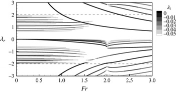
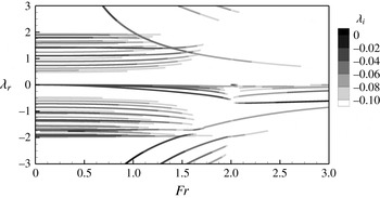
Global stability results using stress-free boundary conditions and
 $Ek=10^{-4}$
are shown in figure 2. The evolution of the frequency
 ${\it\lambda}$
of the different eigenmode solutions is shown as a function of
 $Fr$
for
 $m=2$
and
 $a=0.5$
. A large range of
 $Fr$
, including both ‘wet’ (
 $Fr<2$
) and ‘dry’ (
 $Fr>2$
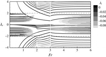
) cases, is shown here, and the associated damping rate is illustrated by means of grey levels, where the darker branches are the least damped modes. The unwetting transition is clearly visible at
 $Fr=2$
, where most of the branches are discontinuous.
Evolution of the eigenvalues with
 $Fr$
for
 $m=2$
,
 $a=0.5$
,
 $Ek=10^{-4}$
and no-stress boundary conditions on the walls. The dashed lines indicate the transitions between hyperbolic and elliptic areas as predicted by the Poincaré equation (3.2).

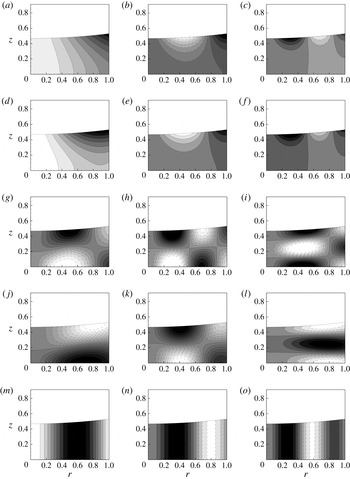
Structures of some eigenmodes obtained numerically for
 $m=2$
,
 $a=0.5$
,
 $Ek=10^{-4}$
,
 $Fr=0.5$
. The pressure component is shown with homogeneously distributed levels, negative contours are dashed. (a)
 $G_{0}$
;
 ${\it\lambda}_{r}=4.290$
,
 ${\it\lambda}_{i}=-0.001416$
; (b)
 $G_{1}$
;
 ${\it\lambda}_{r}=7.436$
,
 ${\it\lambda}_{i}=-0.009232$
; (c)
 $G_{2}$
;
 ${\it\lambda}_{r}=9.043$
,
 ${\it\lambda}_{i}=-0.02008$
; (d)
 $G_{0}^{-}$
;
 ${\it\lambda}_{r}=-5.201$
,
 ${\it\lambda}_{i}=-0.00239$
; (e)
 $G_{1}^{-}$
;
 ${\it\lambda}_{r}=-7.458$
,
 ${\it\lambda}_{i}=-0.00949$
; (f)
 $G_{2}^{-}$
;
 ${\it\lambda}_{r}=-9.035$
,
 ${\it\lambda}_{i}=-0.0202$
; (g)
 $I_{11}$
;
 ${\it\lambda}_{r}=1.408$
,
 ${\it\lambda}_{i}=-0.008326$
; (h)
 $I_{12}$
;
 ${\it\lambda}_{r}=1.098$
,
 ${\it\lambda}_{i}=-0.01326$
; (i)
 $I_{21}$
;
 ${\it\lambda}_{r}=1.785$
,
 ${\it\lambda}_{i}=-0.02265$
; (j)
 $I_{10}^{-}$
;
 ${\it\lambda}_{r}=-1.698$
,
 ${\it\lambda}_{i}=0.006409$
; (k)
 $I_{11}^{-}$
;
 ${\it\lambda}_{r}=-1.330$
,
 ${\it\lambda}_{i}=-0.009475$
; (l)
 $I_{20}^{-}$
;
 ${\it\lambda}_{r}=-1.915$
,
 ${\it\lambda}_{i}=-0.01897$
; (m)
 $R_{0}$
;
 ${\it\lambda}_{r}=-0.03720$
,
 ${\it\lambda}_{i}=-0.002170$
; (n)
 $R_{1}$
;
 ${\it\lambda}_{r}=-0.01417$
,
 ${\it\lambda}_{i}=-0.006563$
; (o)
 $R_{2}$
;
 ${\it\lambda}_{r}=-0.007523$
,
 ${\it\lambda}_{i}=-0.01297$
.

The first point to notice is that all the obtained eigenmodes have a negative growth rate, meaning that the solid body rotation is stable in the range of parameters considered in this case. It turns out that investigations done for other values of the parameters
 $a$
and
 $m$
lead to the same general picture, also with only stable solutions (see figure 12 for
 $m=10$
and
 $a=0.5$
, for instance). So, even though we do not have a rigorous demonstration of this point, we believe that our result allow us to conclude that the solid-body rotation is a stable configuration with respect to modal disturbances in the viscous case. This is in agreement with the historical argument of Newton, which relies on the fact that, in the rotating frame, after a transient stage, the fluid remains perfectly still.
Moreover, it is clear from figure 2 that, for low
 $Fr$
at least, we recover a classification including the three families of waves predicted by the discussion of the Poincaré equation and the shallow-water solutions in the inviscid case, i.e. the frequency ranges
 $|{\it\lambda}|>2$
,
 $|{\it\lambda}|<2$
and
 ${\it\lambda}\approx 0$
indeed correspond to particular sets of solutions. Results are shown here with
 $T_{{\it\Omega}}$
as the time scale for non-dimensional frequencies. This choice implies that inertial waves remains nearly independent of
 $Fr$
(at least for moderate
 $Fr$
) while the frequencies associated with gravity waves diverges as
 $Fr$
goes to zero. Using
 $T_{g}$
allows one to visualize more clearly gravity-driven solutions, as shown, for instance, in figure 4. The typical structures of the different families of waves are shown in figure 3 for
 $Fr=0.5$
and
 $m=2$
, for which the deformation of the free surface is relatively small. In the following, each wave family will be examined in detail using both the finite-element method and an asymptotic study at low Froude number to get an insight into the structure of the different kinds of waves, classify them and study their evolution with
 $Fr$
. The wet case is examined first, since it highlights the simplest configuration for which the three main families of solutions are observed and easily recognized. After that, the high-
 $Fr$
regime, which roughly corresponds to the ‘dry’ case, will be examined in more detail, with specific attention on the transition at
 $Fr=2$
.
4.2. The wet regime
4.2.1. Gravity waves
The low-Froude-number limit allows us to conduct an asymptotic analysis considering that the free surface remains flat (see details in § B.1). In that case, using appropriate expansions and scalings suited for the gravity waves, the Poincaré equation reduces at leading order to a Laplace equation whose solutions are of the form
 $$\begin{eqnarray}p_{0}(r,z)=\cosh (kz)\text{J}_{m}(kr),\end{eqnarray}$$
with
 $\text{J}_{m}$
the Bessel function of the first kind of order
 $m$
and
 $k$
given by the boundary condition as
 $k=j_{mn}^{\prime }$
, i.e. the
 $n$
th root of
 $\text{J}_{m}^{\prime }$
. The boundary condition at the free surface then leads to the classical dispersion relation for gravity waves in finite depth, whose dimensional form reads
 $$\begin{eqnarray}\displaystyle {\it\omega}_{0}=\pm \sqrt{gk\tanh (kH)}. & & \displaystyle\end{eqnarray}$$
Note that, in the case of thin layers, this solution becomes equivalent to the shallow-water solutions found in the low-Froude-number limit, as discussed in § 3.2.
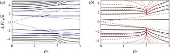
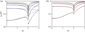
Rescaled frequencies of the gravity waves as function of the Froude number. (a)
 $m=2$
,
 $a=0.5$
: numerical results with
 $Ek=10^{-4}$
and no-stress boundary conditions (plain lines); comparison with the asymptotic results at low
 $Fr$
(blue dashed curves):
 ${\it\lambda}_{0}+{\it\lambda}_{1}Fr/\sqrt{2}$
with
 ${\it\lambda}_{0}$
and
 ${\it\lambda}_{1}$
from table 3 in appendix B. (b)
 $m=1$
,
 $a=0.1$
: numerical results with
 $Ek=10^{-4}$
and no-stress boundary conditions (plain black lines); comparison with general shallow-water solutions detailed in § A.1 (red dashed curves). In both plots, the straight dashed lines starting from the origin indicate the hyperbolic/elliptic region of Poincaré equation in the inviscid case.

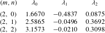
Figure 4(a) compares the evolution of the gravity wave frequencies (rescaled with
 $T_{g}$
here) as obtained by the global stability analysis to the asymptotic predictions (at order
 $2$
). One can note that the asymptotic results give an excellent prediction for
 $Fr\leqslant 1$
, especially for the set of retrograde waves with
 ${\it\lambda}<0$
. Also, the obtained solutions lie in the elliptic region (at least while
 $Fr$
remains moderate) and thus correspond to regular solutions of the Poincaré equation. This is in agreement with the leading-order structure of the pressure field given by (4.1) and the structure shown in figure 3 (a–c) which describe a structure both oscillating along
 $r$
and evanescent along
 $z$
. The integer
 $n$
is chosen so as to correspond to the number of pressure nodes in the radial direction, and we will name the gravity waves
 $G_{n}$
after this integer, with a minus sign exponent for retrograde waves (see figure 3
a–f).
A comparison with the shallow-water solutions is shown in figure 4(b) for moderate
 $a$
(
 $m=1$
and
 $a=0.1$
here). One can observe that, for this value of
 $a$
, the agreement between the two methods is remarkable for small
 $n$
(say
 $|n|<2$
here), as their associated radial wavelength remains large compared to the water depth, a necessary condition for the shallow-water approximation to hold. As
 $|n|$
increases, the results associated with both methods therefore become less accurate.
Structure of the first gravity wave for various
 $Fr$
,
 $m=2$
,
 $a=0.5$
and
 $Ek=10^{-4}$
. (a)
 $G_{0}$
,
 $Fr=1$
;
 ${\it\lambda}_{r}=2.029$
,
 ${\it\lambda}_{i}=-0.001281$
; (b)
 $G_{0}$
,
 $Fr=1.5$
;
 ${\it\lambda}_{r}=1.337$
,
 ${\it\lambda}_{i}=-0.002114$
; (c)
 $G_{0}$
,
 $Fr=1.9$
;
 ${\it\lambda}_{r}=1.061$
,
 ${\it\lambda}_{i}=-0.002173$
.

Finally, one can observe that, prior to dewetting (
 $Fr<2$
), some gravity branches enter the hyperbolic area as
 $Fr$
increases. For instance, this transition for
 $G_{1}$
occurs at
 $Fr\approx 1.1$
for
 $m=2$
and
 $a=0.5$
(see figure 2
a). The precise number of gravity branches featuring such a behaviour is in fact dependent on
 $a$
and
 $m$
(see figure 4). For instance, only
 $G_{1}$
is observed to feature such behaviour in a shallower case with
 $a=0.1$
and for
 $m=1$
(see figure 2
b).
Figure 5 along with figure 3(a) show the evolution of the spatial structure of
 $G_{0}$
for a range of
 $Fr$
, including the above-mentioned transition and for
 $m=2$
and
 $a=0.5$
. It can be seen that, as
 $Fr$
increases, the structure of the wave tends to localize close to the corner formed by the free surface and the outer wall. This corresponds to a transition from an oscillatory trend in the radial direction to an evanescent structure from the wall to the centre. Such eigenmodes are therefore associated with evanescent behaviour in both directions, as expected from the Poincaré solution in the hyperbolic region (see § 3.1). This structure corresponds to that of an edge wave, and has been previously described by Ursell (Reference Ursell1952), for instance. As such edge waves are also systematically observed in the dry case, the discussion of this family is postponed to § 3.1.
4.2.2. Rossby waves
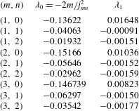
We also start the investigation of the Rossby waves by inspection of the low-Froude-number regime. In contrast to gravity waves, for which the free surface can be considered as flat in this limit, inclusion of free surface variations is essential here. Again the details of the analysis are reported in § B.2. It is found that, at leading order, the velocity components satisfy geostrophic equilibrium, i.e. the Coriolis acceleration is balanced by the pressure gradient. It is further shown that the pressure component at leading order is independent of the vertical direction and reads
 $$\begin{eqnarray}\displaystyle p_{0}(r)=\text{J}_{m}(kr), & & \displaystyle\end{eqnarray}$$
with
 $k^{2}=-2m/(a{\it\lambda}_{0})$
, while the wall boundary condition leads to the frequency selection
 $$\begin{eqnarray}\displaystyle {\it\lambda}=-\frac{2m}{j_{mn}^{2}}Fr^{2}+O(Fr^{4}), & & \displaystyle\end{eqnarray}$$
with
 $j_{mn}$
being the
 $n$
th root of the Bessel function
 $\text{J}_{m}$
. Note that this low-Froude-number solution for the Rossby waves is the same as the one found using the shallow-water approximation (see § 3.2). The next term in the expansion, of order
 $Fr^{4}$
, has also been worked out and is given in § B.2. A comparison of this asymptotic prediction (up to order
 $Fr^{4}$
) with the numerical results is shown in figure 6(a) for
 $m=2$
and
 $a=0.5$
, where the rescaled frequencies
 ${\it\lambda}_{r}/Fr^{2}$
are plotted as a function of
 $Fr$
. As observed, the asymptotic solutions collapse on numerical curves up to
 $Fr\approx 1.2$
at least. Note that, from the low-Froude-number expansion (4.4), the Rossby waves are found to exhibit a slow retrograde motion in the rotating frame, which is a well-known feature of atmospheric Rossby waves (see Vallis Reference Vallis2006, for instance). This trend is well supported by numerical results, as shown in figure 6(a).
Rescaled Rossby waves frequencies as function of
 $Fr$
. Same cases as represented on figure 4 i.e.: (a)
 $m=2$
,
 $a=0.5$
: numerical results with
 $Ek=10^{-4}$
and no-stress boundary conditions (plain black lines) and comparison with the asymptotic at low
 $Fr$
(blue dashed lines):
 ${\it\lambda}={\it\lambda}_{0}^{R}Fr^{2}+{\it\lambda}_{1}^{R}Fr^{4}$
with the values given in the table 4 in appendix B; (b)
 $m=1$
,
 $a=0.1$
: numerical results with
 $Ek=10^{-4}$
and no-stress boundary conditions (plain black lines) and comparison with general shallow-water solutions detailed in § A.1 (red dashed lines).

The spatial structures of some typical Rossby waves are shown in figure 3(m–o). In the following, Rossby waves will be labelled using a single integer
 $n$
, corresponding to the number of nodes in the radial direction of the pressure field; figure 3 thus represents Rossby waves
 $n=0$
,
 $1$
and
 $2$
, further called
 $R_{0}$
,
 $R_{1}$
and
 $R_{2}$
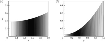
. In particular, one can observe that the vertical independence of the structure (as displayed by the pressure component) predicted by the asymptotic results is striking. Figure 7 displays the structure obtained for
 $R_{0}$
at two values of
 $Fr$
, which shows that the vertical independence persists up to the unwetting point at least. This specific feature allows one to describe Rossby waves using the shallow-water approximation for non-asymptotically small values of
 $a$
(see figure 6
b for
 $a=0.1$
). This stems from the key hypothesis in the shallow-water model presented in § 3.2, which precisely requires that mode structures are vertically independent. The shallow-water approximation is therefore a more useful guide to describe Rossby waves than the Poincaré equation. In particular, the ray-like structure predicted by the latter is not observed in the range of parameters considered here, in contrast to the case of inertial waves (see § 4.2.3). This observation is in agreement with the geophysical field in which Rossby waves are usually described with shallow-water models.
Structure of the first Rossby wave for
 $m=2$
,
 $a=0.5$
and
 $Ek=10^{-4}$
. (a)
 $R_{0}$
,
 $Fr=1$
;
 ${\it\lambda}_{r}=-0.1401$
,
 ${\it\lambda}_{i}=-0.002115$
; (b)
 $R_{0}$
,
 $Fr=1.9$
;
 ${\it\lambda}_{r}=-0.4709$
,
 ${\it\lambda}_{i}=-0.003264$
.

4.2.3. Inertial waves
An asymptotic analysis conducted in the inviscid case at low
 $Fr$
for the inertial waves is detailed in § B.3. In particular, separation of variables allows us to find regular solutions in the case where the free surface remains flat. Such solutions are of the form
 $$\begin{eqnarray}\displaystyle p_{0}(r,z)=\cos (k_{z}z)\text{J}_{m}(k_{r}r), & & \displaystyle\end{eqnarray}$$
where
 $k_{z}$
and
 $k_{r}$
are vertical and radial wave numbers (both real), respectively. The chosen solution (4.5) already satisfies the boundary condition at the bottom of the tank, while boundary conditions imposed at the flat free surface and on the vertical wall lead to two discretization conditions involving integers
 $n_{z}$
and
 $n_{r}$
(see appendix B for details). These discretization conditions, along with the relation (3.5) between
 $k_{z}$
,
 $k_{r}$
and
 ${\it\lambda}$
, lead to the eigenmodes frequencies. In particular, it is found that there is a discrete set of eigenvalues
 ${\it\lambda}_{n_{z},n_{r}}$
which fill the interval
 $[-2,2]$
densely. In the following, inertial waves are labelled as
 $I_{n_{z}n_{r}}$
and
 $I_{n_{z}n_{r}}^{-}$
for cograde and retrograde inertial waves, respectively. Again, the two integers are defined so as to correspond to the number of pressure nodes of the solution in the vertical and radial directions, respectively (see figure 3).
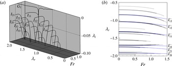
Inertial waves as function of
 $Fr$
for
 $m=2$
,
 $a=0.5$
,
 $Ek=10^{-4}$
and no-stress boundary conditions on the walls. (a) Set of cograde inertial waves: eigenvalues of the least damped modes. (b) Set of retrograde inertial waves: comparison between the numerical results (levels of grey) and the asymptotic trends in the low
 $Fr$
regime (dotted blue lines) given by
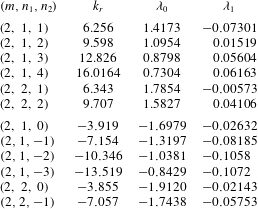
 ${\it\omega}={\it\lambda}_{0}+{\it\lambda}_{1}Fr^{2}/2$
with
 ${\it\lambda}_{0}$
and
 ${\it\lambda}_{1}$
taken from table 5 in appendix B.

Structure of the inertial wave
 $I_{12}$
for various
 $Fr$
,
 $m=2$
,
 $a=0.5$
and
 $Ek=10^{-4}$
. (a)
 $I_{12}$
,
 $Fr=1$
;
 ${\it\lambda}_{r}=1.114$
,
 ${\it\lambda}_{i}=-0.01604$
; (b)
 $I_{12}$
,
 $Fr=1.5$
;
 ${\it\lambda}_{r}=1.198$
,
 ${\it\lambda}_{i}=-0.03263$
; (c)
 $I_{12}$
,
 $Fr=1.9$
;
 ${\it\lambda}_{r}=1.446$
,
 ${\it\lambda}_{i}=-0.2741$
.

When viscosity is added, the dense set of singular inertial waves found in the inviscid case is now unfolded in the complex plane (see the 3-D representation of figure 8(a) for
 $m=2$
and
 $a=0.5$
and
 $Fr<1.3$
). All of the inviscid solutions still exist, but modes having a complex structure generally correspond to a larger damping rate. Therefore, only the least damped modes, which usually correspond to small
 $(n_{z},n_{r})$
, could possibly play an important role in a viscous system. From the numerical results, the spatial structures of these least damped modes can be extracted. In particular, regular inertial waves corresponding to
 $I_{11}$
,
 $I_{12}$
and
 $I_{21}$
(resp.
 $I_{10}^{-}$
,
 $I_{11}^{-}$
and
 $I_{20}^{-}$
) are shown in figure 3 (g–i) (resp. j–l) for
 $m=2$
,
 $a=0.5$
and
 $Fr=0.5$
. One can observe that the structure of the waves is oscillatory in both radial and vertical directions, as expected from the previous discussion of the Poincaré equation. Moreover, the spatial structure is shown to be mostly regular for this value of
 $Fr$
, and indeed resembles the solution of the form (4.5). This comparison between numerical results and asymptotic expansion is highlighted in figure 8(b), in which the frequency
 ${\it\lambda}$
obtained from numerical results for retrograde inertial waves (solid lines with grey levels to indicate damping rate) is compared against asymptotic results (dotted blue lines) as a function of
 $Fr$
for
 $m=2$
and
 $a=0.5$
. It is thus shown that the regular solutions obtained from the asymptotic expansion match numerical results very well up to
 $Fr=0.7$
, at least for this set of parameters. Again, this agreement supports the fact that the spatial structure of inertial waves shows regular patterns in this range of
 $Fr$
numbers.
As
 $Fr$
is increased, the free surface departs substantially from a flat shape. The regular structures of the mode previously described is replaced by patterns which gradually evolve to more complex spatial structures (see figure 9 in which the inertial wave
 $I_{12}$
is tracked as a function of
 $Fr$
). Separation of variables is no longer possible and the dissipative ray-like structure associated with the hyperbolic nature of the inviscid equations in complex geometries arises, as already discussed in § 3.1. Note that the ray structures are not so clear in figure 9 due to the somewhat large value of
 $Ek$
. For this reason, examples of inertial modes structures are shown on figure 10 for
 $Ek=10^{-7}$
. For this value of the Ekman number, solutions clearly exhibit a ray-like spatial structure and the angle between the rays and the rotation axis appears to be in agreement with the predictions from the Poincaré equation (
 $\tan {\it\phi}=\pm 1/\sqrt{4/{\it\lambda}^{2}-1}$
, see § 3.1). The spatial structure of two modes having eigenfrequencies which are close in the complex plane is shown in figure 10(b,c), and it can be seen that these two modes indeed exhibit ray-structures having similar orientations. As
 $Fr$
is further increased, inertial waves slowly disappear as their damping is strongly increased (see figure 8
a, for instance). The physically relevant eigenmodes then become difficult to track numerically, because their damping rates become comparable to those of the spurious numerical modes often encountered in global stability studies.
Example of inertial waves structures for
 $m=2$
,
 $a=0.5$
and
 $Ek=10^{-7}$
. (a)
 $Fr=1$
;
 ${\it\lambda}_{r}=0.9957$
,
 ${\it\lambda}_{i}=-0.001606$
; (b)
 $Fr=1.5$
;
 ${\it\lambda}_{r}=1.493$
,
 ${\it\lambda}_{i}=-0.01606$
; (c)
 $Fr=1.5$
;
 ${\it\lambda}_{r}=1.501$
,
 ${\it\lambda}_{i}=-0.01550$
.

Finally, note that inertial waves can interact with gravity waves when the Froude number gets high enough to allow the latter to enter the hyperbolic region, and thus become edge waves. Such interactions can be seen in figure 2, for instance, and are possible if their respective complex frequencies are close enough. However, it has been found that no instability occurs from these interactions. Here, interactions lead to identity exchange between the two branches of solutions.
As viscosity tends to zero, the structure of the inertial modes is expected to tend towards inviscid attractors which can be constructed using ray-tracing (Maas & Harlander Reference Maas and Harlander2007). In a situation where the flow is periodically forced, the existence of such attractors can lead to strong focusing of the energy, and possibly to an instability due to nonlinear interactions with other secondary waves (Manders & Maas Reference Manders and Maas2004; Jouve & Ogilvie Reference Jouve and Ogilvie2014). However, in the absence of forcing these modes are always much more damped than waves of the two other families described previously. A detailed investigation of the way in which the attractors are approached by the viscous solutions, including scaling laws for the thickness of the shear layers and the damping rate as function of the Eckman number, is clearly out of the scope of the present paper, and left for future studies.
4.3. The dry regime
When
 $Fr>2$
, a dry area of non-dimensional radius
 $r_{c}$
appears at the centre of the cylinder, as shown in figure 1. This transition is associated with the appearance of a new ‘inner’ contact line at the bottom disk. This strong modification affects the different wave families detailed in the previous section, as will be discussed in the following. First, the gravity waves all tend to enter the hyperbolic range, and thus become edge waves. The presence of the dry region also allows the existence of a new class of solution, mostly driven by centrifugal acceleration, and thus called centrifugal waves. Note finally that the Rossby waves have their equivalent in the dry regime (see figure 2, for instance), and are still characterized by vertical independence (see figure 11
b). The nature of this family is therefore not clearly modified from one regime to the other. For this reason, these waves will not be discussed in further detail in the dry case.
Example of structures in the dry regime for
 $m=2$
,
 $a=0.5$
,
 $Ek=10^{-4}$
and
 $Fr=2.5$
. (a)
 $G_{1}$
;
 ${\it\lambda}_{r}=0.8107$
,
 ${\it\lambda}_{i}=-0.001755$
; (b)
 $R_{1}$
;
 ${\it\lambda}_{r}=-0.3261$
,
 ${\it\lambda}_{i}=-0.01162$
; (c)
 $C_{1}^{-}$
;
 ${\it\lambda}_{r}=-0.6727$
,
 ${\it\lambda}_{i}=-0.002466$
.

4.3.1. Edge waves
Non-rotating tanks closed at one edge by a sloping beach are known to support a particular type of gravity waves called edge waves. These waves are well known in coastal dynamics, as they can be observed close to the shoreline. The first partial description of these waves is due to Stokes (Reference Stokes1846), who derived the dispersion relation
 $$\begin{eqnarray}\displaystyle {\it\omega}^{2}=g_{\bot }k\sin ({\it\alpha}), & & \displaystyle\end{eqnarray}$$
where
 ${\it\alpha}$
corresponds to the angle between the free surface and the sloping beach,
 $g_{\bot }$
is the acceleration contribution perpendicular to the free surface (gravity in coastal applications) and
 $k$
the wavenumber in the direction along the edge. Solutions of this dispersion relation are thus called Stokes edge waves. The derivation of Stokes assumes a semi-infinite triangular domain of slope
 ${\it\alpha}$
; but as the waves get increasingly localized as
 $k$
is increased, this expression is expected to hold whatever the shape of the beach away from the edge in the limit
 $k\gg 1$
.
Ursell (Reference Ursell1952) showed that these waves are actually the first of a more general class, whose frequencies are still given by (4.6) but with
 ${\it\alpha}$
replaced by
 $(2n+1){\it\alpha}$
, where
 $n$
is a positive integer such that
 $(2n+1){\it\alpha}<{\rm\pi}/2$
.
In § 4.2.1, we observed that, as the Froude number is increased, some of the gravity wave branches tend to enter the hyperbolic range, and that their structure evolves towards a strong localization at the upper corner of the fluid region (see the structure of
 $G_{0}$
in figure 5). The global results of figure 2 also show that other branches enter the hyperbolic area for
 $Fr>2$
. We thus expect to be able to describe these waves with the same approach as Stokes (Reference Stokes1846) and Ursell (Reference Ursell1952).
In the present case, the direction along the edge is the azimuthal direction, so the wavenumber
 $k$
appearing in (4.6) has to be replaced by
 $m/R$
, and the condition that the wave is localized at the edge actually implies
 $m\gg 1$
. Under that assumption, the free surface can be approximated as flat, with a slope
 ${\it\alpha}$
with respect to the lateral wall given by
 $\tan {\it\alpha}=1/h^{\prime }(R)\equiv 1/(aFr^{2})$
. The acceleration perpendicular to the surface in (4.6) has to be replaced by the equivalent acceleration at the edge, i.e.
 $g_{\bot }=g_{e}(R)$
. Finally, we account for the rotation by replacing the frequency
 ${\it\omega}$
in (4.6) by the relative frequency
 ${\it\omega}-m{\it\Omega}$
, and neglect all curvature effects. We are thus led to the following prediction for the frequencies of edge waves
 $$\begin{eqnarray}({\it\omega}-m{\it\Omega})^{2}=g_{e}(R)\frac{m}{R}\sin [(2n+1){\it\alpha}],\end{eqnarray}$$
in which
 $n$
is a positive integer satisfying
 $(2n+1){\it\alpha}\leqslant {\rm\pi}/2$
. In particular, only one solution is allowed for
 ${\it\alpha}\approx {\rm\pi}/2$
(i.e. for small
 $Fr$
), whereas an increasing number of solutions are obtained when
 ${\it\alpha}$
gets smaller (i.e. when
 $Fr$
increases). The solution
 $n=0$
is the equivalent Stokes edge wave solution, which simply reads
 $({\it\omega}-m{\it\Omega})^{2}=gm/R$
(
 ${\it\lambda}_{r}^{2}=m/(aFr^{2})$
in non-dimensional form). The structure of this wave is depicted in figure 11(a) in a dry case corresponding to
 $a=0.5$
and
 $Fr=2.5$
. It can be seen from the pressure component that the wave is indeed trapped at the upper edge.
Figure 12 compares the predictions of the model (4.7) with the global results for
 $m=10$
, a high value where the edge wave model is expected to be most accurate. As can be seen, the Stokes wave solutions (with
 $n=0$
) nicely fit
 $G_{0}$
and
 $G_{0}^{-}$
in the case
 $a=0.5$
and
 $m=10$
. The edge waves with
 $n=1$
and
 $n=2$
are also displayed, and are shown to be in good accordance with the next branches of gravity waves which successively enter the hyperbolic region as
 $Fr$
is increased.
4.3.2. Centrifugal waves
Another kind of wave that is not present prior to dewetting is now reported. After the transition at
 $Fr=Fr_{c}$
, an additional contact line appears at the bottom of the tank, allowing a new family of wave solutions. As will be seen, the restoring force associated with these waves corresponds to the centrifugal acceleration, and we therefore call them centrifugal waves. This kind of wave is more classically encountered in the case of a hollow core vortex in solid body rotation, which in fact is equivalent to the present configuration with an additional top wall and in the limit of infinite Froude number. This case will be studied further in § 6 (see also appendix C), where a proper introduction of centrifugal waves is presented.
Evolution of the eigenvalues with
 $Fr$
for
 $m=10$
,
 $a=0.5$
,
 $Ek=10^{-4}$
and no-stress boundary conditions on the walls. The circles correspond to the frequencies of the couple of 2-D centrifugal waves given by (4.8) and crosses correspond to edge waves obtained from dispersion relation (4.7) for
 $n=0,1,2$
.

In this section we only report the results obtained for the 2-D centrifugal waves which are of particular interest in the dry case. From the derivation reported in appendix C, and considering that we are close to the dewetting point (
 ${r_{c}}^{2m}\ll 1$
), the dispersion relation for 2-D centrifugal waves can be written as
 $$\begin{eqnarray}{\it\lambda}_{C^{\pm }}\approx 1\pm \sqrt{1+m}.\end{eqnarray}$$
In dimensional form this reads
 ${\it\omega}\approx (m+1){\it\Omega}\pm \sqrt{g_{c}k_{c}}$
, with
 $g_{c}=r_{c}{\it\Omega}^{2}$
the local centrifugal acceleration at the inner contact line and
 $k_{c}=(m+1)/r_{c}$
an equivalent radial wave number. This dispersion relation is analogous to that of classical surface waves under the infinite depth approximation, and these waves therefore correspond to surface waves driven by centrifugal acceleration. An example of such a centrifugal wave is displayed in figure 11(c), where it can be seen that the wave is trapped close to the inner contact line.
The prediction of those waves allows us to understand some important
 $Fr$
-independent features, as seen, for instance, in figure 12 for
 $m=10$
and
 $a=0.5$
in the dry regime. In particular, open symbols in figure 12 correspond to the solution (4.8), and it can be seen that these solutions are indeed associated with the appearance of new waves at
 ${\it\lambda}_{r}\approx -2.3$
and
 ${\it\lambda}_{r}\approx 4.3$
in the global stability results. For this value of
 $m$
, both waves are found to be in the elliptic area, but (4.8) shows that 2-D centrifugal waves can also exist in the hyperbolic region for smaller
 $m$
.
4.4. Transition from wet to dry cases
Figure 2, among others, showed that many wave branches display a singular behaviour with a change of slope at
 $Fr=Fr_{c}=2$
. Such a singularity is not surprising, considering that the dewetting transition sharply modifies the boundary condition at the inner part of the domain. This singular behaviour can be observed on most of the gravity waves, especially for small aspect ratios (see figure 4(b) for
 $a=0.1$
), and Rossby waves (see figure 6). In order to characterize this transition, we have conducted an asymptotic analysis, valid for
 $|Fr-Fr_{c}|\ll 1$
, based on the shallow-water approximation. Details are reproduced in § A.3. Here we summarize only the main predictions of this study:
-
(i) There is only one branch which remains regular at the wet–dry transition. For
 $Fr=2$
the frequency of this wave is denoted as
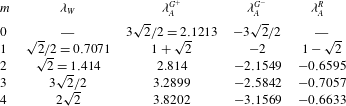
${\it\lambda}_{W}=m/\sqrt{2}$
. The structure of this wave is non-oscillatory in the radial direction.
-
(ii) All the other branches are singular, and belong to three families, which all follow a law of the form
(4.9)where
$$\begin{eqnarray}\displaystyle {\it\lambda}\approx {\it\lambda}_{A}+O(\log |Fr-Fr_{c}|^{-2}), & & \displaystyle\end{eqnarray}$$
${\it\lambda}_{A}$
takes three possible values, noted
${\it\lambda}_{A}^{G+}$
, (for cograde gravity waves),
${\it\lambda}_{A}^{G-}$
, (for retrograde gravity waves), and
${\it\lambda}_{A}^{R}$
(for Rossby waves). The structure of these waves is oscillatory in the radial direction and localized in the vicinity of the centre.


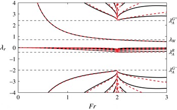
To illustrate this transition, the different branches obtained from shallow-water solutions and numerical solutions are shown as a function of
 $Fr$
for
 $a=0.1$
and
 $m=1$
in figure 13. The results in this case fully confirm the predictions of the asymptotic study. First, we observe that a single branch has a regular behaviour and passes through
 ${\it\lambda}_{W}$
for
 $Fr=2$
. This branch corresponds to the cograde gravity wave with the simplest structure, which was termed
 $G_{0}$
in § 4.2.1. Second, we observe that all the other branches effectively have a common limit, which is either
 ${\it\lambda}_{A}^{G+}$
,
 ${\it\lambda}_{A}^{G-}$
, or
 ${\it\lambda}_{A}^{R}$
for the three families of waves. Finally, we observe that the approach towards this limit is very sharp, in accordance with the logarithmic behaviour predicted by the asymptotic analysis.
Dispersion curves obtained in the shallow-water regime for
 $m=1$
,
 $a=0.1$
: shallow-water equation (dashed red lines), global stability approach with
 $Ek=10^{-4}$
and no-stress boundary conditions on the walls (black). The horizontal dashed lines correspond to the frequencies coming from the mathematical analysis at the transition
 $Fr=Fr_{c}$
(see discussion in text).

Let us now briefly discuss the wet–dry transition at larger aspect ratios. For this, we go back to the case
 $(m=2,a=0.5)$
presented in figure 2. Although the transition at
 $Fr=2$
is not as sharp as previously described, the asymptotic predictions presented above still capture part of the observed behaviour. However, although most of the waves display a change of behaviour, with a steep slope reminiscent of the logarithmic singularity, they do not tend to accumulate towards a single limit (
 ${\it\lambda}_{A}^{G+}$
,
 ${\it\lambda}_{A}^{G-}$
,
 ${\it\lambda}_{A}^{R}$
) for each family. Another difference is that, in contrast to the asymptotic prediction, there is not a single branch which remains regular at the wet–dry transition. For instance, in figure 2, four branches of gravity waves remain regular. One can explain this feature by recalling that, in this range of Froude numbers, the gravity waves tend to become edge waves localized in the vicinity of the upper corner, so the change in nature of the boundary condition at the inner part of the domain has less effect on their structure.
5. Effect of the wall conditions
All the results shown until now have been obtained using no-stress boundary conditions on the solid walls. This simplification allows one to have a clear view of the wave structures in the bulk and to make proper comparisons with inviscid analytical results. However, wall boundary layers are expected to affect the present results, and it would be useful to know if these results remain relevant in a more realistic case where no-slip conditions are considered. For this purpose, global stability results are computed in the no-slip case using an analogous method as presented in § 2.3, but with Dirichlet boundary conditions on the bottom and side walls. Note that the contact lines (upper and also inner for
 $Fr>Fr_{c}$
) are considered pinned, i.e. the triple line is anchored at the base state position in the present case.
Same as figure 2 (
 $a=0.5$
,
 $m=2$
) in the no-slip case.

Figure 14 shows the results obtained under the same conditions as for figure 2, but for no-slip conditions on the walls. Comparison between figures 14 and 2 therefore gives some indications regarding the effect of the no-slip condition. First, it seems clear that we obtain the same general picture regarding the evolution of the eigenmode frequencies with the Froude number. The frequencies are in fact very close, because the leading order is driven by the inviscid solution. However, in the no-slip case, an additional damping is found due to the dissipative contributions in the wall boundary layers associated with such a boundary condition.
It can be observed in figure 14 that the wave families are not affected in the same way by this change of wall conditions. In particular, the damping rates of the inertial waves are less affected than other families. This can be understood by considering the structures of the waves as described in the previous section, leading in the case of the inertial wave to a bulk dissipation, while wall effects are expected to be more important for gravity and Rossby waves. The importance of bulk dissipation for inertial waves has already been observed in previous studies, such as the case of a fluid in a rotating cylinder (see, for instance, Eloy et al. Reference Eloy, Le Gal and Le Dizès2003).
Finally, it can be noted that an influence of the Froude number on the damping rate is clearly highlighted for the gravity waves. In particular, the damping increases for increasing
 $Fr$
for no-slip boundary conditions (figure 14), while this behaviour was less obvious for the no-stress condition (figure 2) in the range of parameters considered here. For instance, the damping rate of the mode
 $G_{0}$
goes from
 $|{\it\omega}_{i}|\approx 0.02$
for
 $Fr\approx 0.6$
to less than
 $0.1$
for
 $Fr=3$
. This trend can be attributed to a growth of the wall surface in contact with the fluid with increasing
 $Fr$
. This trend is not observed for inertial waves which have a spatial structure which tends to a ray-like pattern for increasing
 $Fr$
. Most of the dissipation is then expected to take place in these shear layers, the volume dissipation being once again the most important for this wave family. Compared with Rossby waves, gravity waves tend to be concentrated close to the outer contact line (edge waves). Hence, we suspect that the influence of
 $Fr$
when the no-slip condition is applied on the walls (and in particular on the cylinder) will more strongly affect the structure of gravity waves.
The main conclusion of this section is that frequencies obtained in the no-stress cases seem to match at first order with the no-slip case for the entire range of
 $Fr$
considered. Therefore, the results obtained in the previous section considering no-stress boundary conditions remain relevant and of interest for more realistic configurations. This observation is consistent with the fact that the restoring forces involved with the different wave families found here are inviscid processes.
6. Effect of a top wall
Up to now, we have considered that the rotating container is high enough such that the liquid never reaches the top of the vertical wall. We now consider the case where the container has a finite height
 $H_{t}$
. This situation leads to the introduction of an additional geometrical parameter, namely
 $a_{t}=H_{t}/R$
. A full description of this case is clearly out of the scope of the present paper, so we will restrict the discussion here to an illustration of the effect of the top wall for the single case
 $a=0.5$
,
 $a_{t}=1.5$
.
The results of the previous sections still hold up to the point where the free surface reaches the top wall. Inspection shows that this case happens for a critical Froude number
 $Fr_{ct}$
defined as
 $$\begin{eqnarray}\displaystyle Fr_{ct}=\frac{a_{t}}{a}. & & \displaystyle\end{eqnarray}$$
Up to
 $Fr_{ct}$
, the mean shape of the free surface is still given by (2.4). For
 $Fr>Fr_{ct}$
, the mean shape is now given by
 $$\begin{eqnarray}\displaystyle h(r)=\frac{aFr^{2}}{2}(r^{2}-r_{c}^{2})\quad \text{for }r_{c}<r<r_{ct}, & & \displaystyle\end{eqnarray}$$
where
 $r_{c}$
and
 $r_{ct}$
are the radii of the dry regions on the bottom and top plates, given by
 $$\begin{eqnarray}\displaystyle r_{c}=\sqrt{\frac{a_{t}-a}{a_{t}}-Fr^{-2}\frac{a_{t}}{a}},\quad r_{ct}=\sqrt{\frac{a_{t}-a}{a_{t}}+Fr^{-2}\frac{a_{t}}{a}}. & & \displaystyle\end{eqnarray}$$
In the limit
 $Fr\approx \infty$
, where the gravity becomes negligible with respect to the centrifugal acceleration, the free surface becomes vertical, and the situation corresponds to a rotating fluid with a cylindrical hollow core of radius
 $r_{cm}=\sqrt{1-a/a_{t}}$
. Interestingly, in this situation, one recovers the possibility of an analytical resolution in separated form, and we therefore expect to find the existence of regular inertial waves. This situation was actually investigated in previous works (Sun Reference Sun1960; Miles & Troesh Reference Miles and Troesh1961; Ibrahim Reference Ibrahim2005). We reproduce the details of the analytical treatment in appendix C. Here we give only a summary of the predictions for this case:
-
(i) First, there exist two waves with a 2-D structure (independent of
$z$
) which are driven by centrifugal acceleration at the free surface. These waves are the same as previously encountered in § 4.3.2 when the top wall is not reached, and their dimensionless frequency now reads (6.4)Note that these waves may lie either in the hyperbolic or elliptic ranges, without affecting the structure.
$$\begin{eqnarray}{\it\lambda}=K\pm \sqrt{K(K+m)},\quad \text{with }K=\frac{1-r_{cm}^{2m}}{1+r_{cm}^{2m}}.\end{eqnarray}$$
-
(ii) Second, among the waves with a 3-D structure, we can distinguish a set of waves characterized by
$n_{z}$
nodes in the vertical direction, and no nodes in the radial direction. These waves are denoted here as
$C_{n_{z}}^{\pm }$
, and like the 2-D waves they may lie either in the hyperbolic or elliptic range. -
(iii) Third, the last kind of solutions consists of waves with
$n_{z}$
nodes in the vertical direction and
$n_{r}$
nodes in the radial direction. These waves are called
$I_{n_{z}n_{r}}^{\pm }$
and they always lie in the hyperbolic region.


Note that, strictly speaking, all waves are equally influenced by centrifugal acceleration at the free surface and Coriolis acceleration in the bulk. However, the waves with no radial nodes have a structure mostly localized close to the free surface and can be identified as surface waves driven by centrifugal acceleration, while the other waves with a more complex structure are less influenced by the presence of the free surface and can be related to the inertial waves encountered in § 4.2.3; hence the denomination of the waves proposed above.
Sample result with a top wall (
 $m=2$
,
 $a=0.5$
,
 $a_{t}=1.5$
,
 $Ek=10^{-4}$
). The dashed lines correspond to
 $\pm 2$
and therefore delimit the inviscid range of existence corresponding to inertial waves.

Figure 15 shows an example of the results found in Newton’s bucket with a top wall for
 $a=0.5$
,
 $a_{t}=1.5$
,
 $m=2$
and
 $Ek=10^{-4}$
. Let us inspect the results in the new ‘top’ regime for
 $Fr>Fr_{ct}$
. We clearly distinguish two main kinds of branches. First, the darker branches, which form a regular set and can be followed down to the transition at
 $Fr_{ct}$
, correspond to the centrifugal waves
 $C_{n}^{\pm }$
. Note that for the set of parameters considered, the waves
 $C_{0}^{+},C_{1}^{+},C_{0}^{-},C_{1}^{-}$
and
 $C_{2}^{-}$
belong to the hyperbolic range, while the higher ones all belong to the elliptic range. The second set of branches are the more numerous and more damped waves contained in the hyperbolic range
 ${\it\lambda}\in [-2,2]$
, and correspond to the inertial waves. Most of these branches tend to disappear as the Froude number is decreased towards the transition at
 $Fr_{ct}$
. This feature roughly mirrors the behaviour which was observed in the wet regime as the Froude number is increased towards
 $Fr_{c}$
. The explanation is the same: as the Froude number is decreased, the domain occupied by the fluid departs from the rectangular domain which allows a separated variable solution, and the singularity associated with the Poincaré equation in the hyperbolic case reappears.
Waves in Newton’s bucket with a top wall: comparison between inviscid results in the large-Froude number limit and global viscous results (
 $a=0.5,a_{t}=1.5,m=2$
).

To illustrate the results further, we display in figure 16 the structure of three different waves for a large Froude number, namely
 $Fr=6$
. The three waves displayed, namely
 $C_{0}^{-}$
,
 $C_{2}^{+}$
and
 $I_{31}^{-}$
, are in accordance with the predictions of the inviscid case discussed above. We also show in table 1 a comparison of the frequencies predicted in the inviscid case for
 $Fr\approx \infty$
and computed through the global approach for
 $Fr=6$
. The comparison shows excellent agreement for this value of
 $Fr$
, and also shows that the inertial waves are substantially more damped than the centrifugal waves.
Structure of some waves in the top-wall case for
 $m=2$
,
 $a=0.5$
,
 $a_{t}=1.5$
,
 $Ek=10^{-4}$
,
 $Fr=6$
. (a)
 $C_{0}^{-}$
;
 ${\it\lambda}_{r}=-0.576$
,
 ${\it\lambda}_{i}=-0.00101$
; (b)
 $C_{2}^{+}$
;
 ${\it\lambda}_{r}=2.256$
,
 ${\it\lambda}_{i}=-0.00716$
; (c)
 $I_{31}^{-}$
;
 ${\it\lambda}_{r}=-0.644$
,
 ${\it\lambda}_{i}=-0.0387$
.

Finally, let us briefly discuss the reconnection between the various kinds of waves at the transition between the ‘dry’ and ‘top’ regimes at
 $Fr=Fr_{ct}$
. We can see that, although most branches display a slope discontinuity, the centrifugal branches smoothly reconnect with the surface waves which were discussed in § 4. As we have seen, these surface waves were most easily interpreted as ‘gravity waves’ in the wet regime, while some of them tended to acquire an ‘edge wave’ behaviour in the dry regime. The connection confirms that all these waves – gravity, centrifugal and edge – actually belong to the general class of surface waves. The connection between the branch
 $C_{0}^{-}$
in the top regime and the branch
 $C^{-}$
in the dry regime, which had already been interpreted as a centrifugal waves, is also clear. Finally, we note that the set of branches corresponding to Rossby waves existing in the dry regime can be continued in the top regime. As the Froude number is further increased these branches tend to lose their identity and merge with the set of inertial waves.
7. Summary and conclusions
The solid body rotation of a free surface flow in a confined cylindrical tank has been considered by means of global stability analysis in the viscous case and various asymptotic methods. The stability of this configuration has been confirmed in the viscous case to be in agreement with the famous bucket experiment in which the free surface is perfectly still. However, the analysis unveils the complexity of such a configuration due to the presence of different kinds of waves, namely surface waves (gravity and centrifugal), inertial waves and Rossby waves, which can coexist in an intricate way. In this paper we provide a comprehensive and coherent classification of these waves for a large range of parameters, including wet cases and dry cases, a description of the dewetting transition, and an extension where a top wall is included.
The need for such a classification of waves is rooted in recent studies related to the rotating bottom experiment (fixed lateral wall), where symmetry breaking of the free surface can be seen. Indeed, the flow existing in such an experiment has been found to be described well at first order by a Rankine vortex (Bergmann et al. Reference Bergmann, Tophøj, Homan, Hersen, Andersen and Bohr2011), which therefore incorporates a central core in solid body rotation. Fabre & Mougel (Reference Fabre and Mougel2014) showed, using a simple model composed of two fluid layers, that the presence of the rigidly rotating region offers a possible explanation for the switching phenomenon which can be seen in the rotating bottom experiment (Iga et al. Reference Iga, Yokota, Watanabe, Ikeda, Niino and Misawa2014). However, the present results suggest that many additional waves can interact when the whole volume of fluid is considered, and details regarding the global stability of the Rankine vortex will therefore be the object of further studies to complement the preliminary results of Mougel et al. (Reference Mougel, Fabre and Lacaze2014).
Although the present study has addressed, as exhaustively as possible, the stability of the flow in the viscous case and from a modal point of view, there are necessarily a number of issues which are left aside and could be the object of future studies. First, the effect of viscosity on the various families of waves has been investigated only in a qualitative way, and could certainly be the object of a more thorough study, in order to predict the damping rates of the modes due to viscous dissipation in the boundary layers and within the thin shear layers constituting the inertial modes. Second, we have restricted the discussion here to a description of the unforced case. Investigating the response of the flow to a harmonic forcing is a different problem, which would certainly justify a whole study on its own. In this case, due to the singularity of the inviscid problem in the hyperbolic range, one can expect to observe a geometric instability (Maas & Harlander Reference Maas and Harlander2007) due to the focussing of perturbations towards the attractors of the singular modes. Finally, the present study has disregarded the effects of surface tension. Such effects are expected to lead to two complications. First, the parabolic shape of the free surface is no longer relevant, and one should consider the actual equilibrium shape resulting from both rotation and capillary effects. Second, surface tension is known to give rise to a new family of waves, namely capillary waves, whose interactions with the other families of waves will certainly lead to interesting results.
Appendix A. The shallow-water regime
A.1. General solutions for dry and wet cases
In both dry and wet cases, an appropriate change of variables can reduce (3.7) to a hypergeometric differential equation (see (15.5.1) in Abramowitz & Stegun Reference Abramowitz and Stegun1972). The most convenient change of variables is as follows:
 $$\begin{eqnarray}\displaystyle Z & = & \displaystyle \displaystyle \frac{2Fr^{2}r^{2}}{Fr^{2}-4}\text{ in the wet case},\end{eqnarray}$$
 $$\begin{eqnarray}\displaystyle Z & = & \displaystyle \displaystyle \frac{r^{2}}{r_{c}^{2}}\text{ in the dry case}.\end{eqnarray}$$
 $\mathscr{F}(a,b;c;z)$
and the general solution involves two hypergeometric solutions, which can be expressed in a variety of forms, all listed in Abramowitz & Stegun (Reference Abramowitz and Stegun1972, § 15.5). Here it is found that only one hypergeometric solution is needed. The reason for that is case dependent. In the dry case, regularity, or equivalently (3.9b,c
), at
 $r=0$
prohibits one of the two linearly independent solutions to the second-order equation. In the dry case, it turns out that only one linear solution is needed, as it straightforwardly satisfies boundary condition (3.9b,c
) at
 $r=r_{c}$
. In the wet case, the general solution is of the form
 $$\begin{eqnarray}{\it\eta}(Z)=Z^{|m|/2}\mathscr{F}\left(\frac{1+|m|+\sqrt{M}}{2},\frac{1+|m|-\sqrt{M}}{2};|m|+1;Z\right),\end{eqnarray}$$
while in the dry case, one finds
 $$\begin{eqnarray}{\it\eta}(Z)=Z^{|m|/2}\mathscr{F}\left(\frac{1+|m|+\sqrt{M}}{2},\frac{1+|m|-\sqrt{M}}{2};1;1-Z\right),\end{eqnarray}$$
where we have introduced
 $M=1+m^{2}-2{\it\Lambda}$
, and again,
 ${\it\Lambda}={\it\lambda}^{2}-4-2m/{\it\lambda}$
.
Using boundary condition (3.9b,c
) for both the wet case and the dry case then leads to the dispersion relations
 $\mathscr{D}_{w}({\it\lambda},m)=0$
and
 $\mathscr{D}_{d}({\it\lambda},m)=0$
, respectively, which gives an implicit solution for
 ${\it\lambda}$
.
A.2. Asymptotic expansion for shallow-water solutions
Here we introduce
 $\bar{h}(r)=h(r)/a$
, the reduced height profile given by
 $$\begin{eqnarray}\displaystyle \bar{h}(r)=1+\frac{Fr^{2}}{2}\left(r^{2}-\frac{1}{2}\right)\quad \text{if }Fr<2, & & \displaystyle\end{eqnarray}$$
in the wet case and
 $$\begin{eqnarray}\displaystyle \bar{h}(r)=\frac{Fr^{2}}{2}(r^{2}-r_{c}^{2})\quad \text{if }Fr>2, & & \displaystyle\end{eqnarray}$$
in the dry case.
Using this notation (3.7) can be written as
 $$\begin{eqnarray}{\it\eta}^{\prime \prime }(r)+\left(\frac{1}{r}+\frac{Fr^{2}r}{\bar{h}(r)}\right){\it\eta}^{\prime }(r)+\left(\frac{Fr^{2}{\it\Lambda}}{\bar{h}(r)}-\frac{m^{2}}{r^{2}}\right){\it\eta}(r)=0.\end{eqnarray}$$
This new formulation is slightly more convenient to derive the following asymptotic expansions.
A.2.1. Asymptotic trends for
$Fr\ll 1$

In the low-Froude-number limit, corresponding to the wet case, two kinds of solution have to be considered:
 ${\it\lambda}\ll 1$
(Rossby waves) and
 ${\it\lambda}\gg 1$
(gravity waves). In this limit (A 6) reduces to
 $$\begin{eqnarray}\displaystyle {\it\eta}^{\prime \prime }(r)+\frac{1}{r}{\it\eta}^{\prime }(r)+\left(Fr^{2}{\it\Lambda}-\frac{m^{2}}{r^{2}}\right){\it\eta}(r)=0. & & \displaystyle\end{eqnarray}$$
The two solutions, Rossby waves and gravity waves, then correspond to the expansion
 ${\it\lambda}={\it\lambda}_{0}Fr^{2}+O(Fr^{4})$
and
 ${\it\lambda}={\it\lambda}_{0}Fr^{-1}+O(1)$
, where
 ${\it\lambda}_{0}$
is order one, leading to
 $$\begin{eqnarray}\displaystyle & \displaystyle {\it\eta}^{\prime \prime }(r)+\frac{1}{r}{\it\eta}^{\prime }(r)+\left(-\frac{m^{2}}{r^{2}}-\frac{2m}{{\it\lambda}_{0}}\right){\it\eta}(r)=0, & \displaystyle\end{eqnarray}$$
 $$\begin{eqnarray}\displaystyle & \displaystyle {\it\eta}^{\prime \prime }(r)+\frac{1}{r}{\it\eta}^{\prime }(r)+\left({\it\lambda}_{0}^{2}-\frac{m^{2}}{r^{2}}\right){\it\eta}(r)=0. & \displaystyle\end{eqnarray}$$
Solutions of (A 8) and (A 9) are of the form
 ${\it\eta}=\text{J}_{m}(\sqrt{-2m/{\it\lambda}_{0}}r)$
and
 ${\it\eta}=\text{J}_{m}({\it\lambda}_{0}r)$
, respectively. The inviscid boundary condition at
 $r=1$
leads to the dispersion relations
 $$\begin{eqnarray}\mathscr{D}_{R}^{w}=\text{J}_{m}(\sqrt{-2m/{\it\lambda}_{0}})=0,\quad \text{i.e.}~{\it\lambda}_{0}=-\frac{2m}{j_{mn}^{2}},\end{eqnarray}$$
for Rossby waves and
 $$\begin{eqnarray}\mathscr{D}_{G}^{w}=m\text{J}_{m}({\it\lambda}_{0})-{\it\lambda}_{0}\text{J}_{m+1}({\it\lambda}_{0})=0,\end{eqnarray}$$
for gravity waves, respectively. Note that (A 10) is the leading-order solution derived for Rossby waves in the small-Froude-limit (derived in appendix B).
A.3. Asymptotic trends for
$Fr\approx 2^{-}$

To investigate the wet–dry transition, we introduce
 $Fr=2-{\it\delta}$
and consider the limit
 ${\it\delta}\ll 1$
with
 ${\it\delta}>0$
. This case thus corresponds to approaching the transition from the ‘wet’ side. The mirror case
 $Fr\approx 2^{+}$
with
 ${\it\delta}<0$
is very similar but is not detailed here.
The hypergeometric solution can be written in the form
 $$\begin{eqnarray}{\it\eta}=x^{|m|}\mathscr{F}\left(\frac{m+1+\sqrt{M}}{2},\frac{m+1-\sqrt{M}}{2};|m|+1;\frac{-2r^{2}}{{\it\delta}}\right),\end{eqnarray}$$
with
 $$\begin{eqnarray}\displaystyle M=m^{2}+1-2{\it\Lambda}=\frac{4m}{{\it\lambda}}+(m^{2}+9)-2{\it\lambda}^{2}. & & \displaystyle\end{eqnarray}$$
As
 ${\it\delta}$
tends to zero, the argument in the hypergeometric solution becomes large, so we can use the asymptotic forms corresponding to this case. The situation differs according to the sign of
 $M$
.
A.3.1. Case
$M>0$

In this case, the asymptotic behaviour is (Abramowitz & Stegun Reference Abramowitz and Stegun1972, (15.3.7))
 $$\begin{eqnarray}\displaystyle {\it\eta}\approx Ar^{\sqrt{M}-1}, & & \displaystyle\end{eqnarray}$$
with
 $A$
some arbitrary multiplicative factor. We introduce this behaviour into the boundary condition for
 $r=1$
,
 $$\begin{eqnarray}\displaystyle {\it\lambda}\left(\sqrt{\frac{4m}{{\it\lambda}}+(m^{2}+9)-2{\it\lambda}^{2}}-1\right)-2m=0. & & \displaystyle\end{eqnarray}$$
For each
 $m\neq 0$
, this equation has a single root, denoted
 ${\it\lambda}_{W}=m\sqrt{2}/2$
. Values are given in table 2. This branch is the only regular one in the limit
 $Fr\approx 2$
.
Coefficients entering the asymptotic expressions of the waves for
 $Fr\approx 2^{-}$
.

A.3.2. Case
$M<0$

This case is encountered in three intervals, noted
 $[-\infty ,{\it\lambda}_{A}^{G^{-}}]$
,
 $[{\it\lambda}_{A}^{R},0]$
,
 $[{\it\lambda}_{A}^{G+},\infty ]$
, where the
 ${\it\lambda}_{A}$
s are the three roots of
 $M=0$
. The numerical values for these numbers are given in table 2. The fact that
 $M<0$
leads to an oscillating function
 ${\it\eta}$
, and hence the possibility for a family of waves in each of the intervals. In practice we found that, as
 ${\it\delta}$
tends to zero, the branches accumulate toward the corresponding
 ${\it\lambda}_{A}$
. Thus we start with an expansion of the form
 ${\it\lambda}={\it\lambda}_{A}+{\it\lambda}_{1}$
. We also write
 $M=-{\it\beta}^{2}$
, with
 ${\it\beta}^{2}=-(\partial M/\partial {\it\lambda}){\it\lambda}_{1}$
. Then the asymptotic expression for the hypergeometric function leads to
 $$\begin{eqnarray}\displaystyle {\it\eta}\approx A\left(\frac{\sqrt{2}r}{\sqrt{{\it\delta}}}\right)^{-1+\text{i}{\it\beta}}+\text{c.c.}\equiv A\left(\frac{r}{\sqrt{{\it\delta}}}\right)^{-1}\cos ({\it\beta}\log (r/2\sqrt{{\it\delta}})), & & \displaystyle\end{eqnarray}$$
where
 $\text{c.c.}$
stands for complex conjugate. Imposition of the boundary condition at
 $r=1$
leads to
 ${\it\beta}\log ({\it\delta})=n{\rm\pi}$
. Hence
 ${\it\lambda}_{1}\sim n^{2}/(\log {\it\delta})^{2}$
.
Appendix B. The low-Froude-number regime
In this appendix we investigate the limit of weak rotation. As discussed in the main text, in this case the domain occupied by the fluid reduces to a rectangular cylindrical region, thus allowing a solution with separated variables for each of the three main families of waves. Here we derive this solution using asymptotic developments in powers of the Froude number, which are carried out up to second-order terms for Rossby and inertial waves, and up to third-order terms for gravity waves. For such developments, it turns out to be more convenient to use a different definition for the Froude number, namely
 $$\begin{eqnarray}\displaystyle F={\it\Omega}\sqrt{\frac{R}{g}}=a^{1/2}Fr. & & \displaystyle\end{eqnarray}$$
With this notation, the starting equations read
 $$\begin{eqnarray}\displaystyle & \displaystyle \frac{\partial ^{2}p}{\partial r^{2}}+\frac{1}{r}\frac{\partial p}{\partial r}-\frac{m^{2}}{r^{2}}p+\left(\frac{{\it\lambda}^{2}-4}{{\it\lambda}^{2}}\right)\frac{\partial ^{2}p}{\partial z^{2}}\equiv {\rm\Delta}p-\frac{4}{{\it\lambda}^{2}}\frac{\partial ^{2}p}{\partial z^{2}}=0, & \displaystyle\end{eqnarray}$$
 $$\begin{eqnarray}\displaystyle & \displaystyle \frac{\partial p}{\partial z}-F^{2}{\it\lambda}^{2}p+\frac{F^{2}h_{2}^{\prime }{\it\lambda}}{{\it\lambda}^{2}-4}\left(\frac{2m}{r}p-{\it\lambda}\frac{\partial p}{\partial r}\right)=0\quad \text{for }z=a+F^{2}h_{2}(r), & \displaystyle\end{eqnarray}$$
 $$\begin{eqnarray}\displaystyle & \displaystyle {\it\lambda}\frac{\partial p}{\partial r}-2mp=0\quad \text{for }r=1, & \displaystyle\end{eqnarray}$$
 $h_{2}(r)=r^{2}/2-1/4$
.
Values of the coefficients in the expansion of gravity waves for
 $a=0.5$
.

B.1. Gravity surface waves
For this first family, the eigenvalues are expanded in the following form
 $$\begin{eqnarray}\displaystyle {\it\lambda}=F^{-1}{\it\lambda}_{0}+{\it\lambda}_{1}+F{\it\lambda}_{2}+\ldots . & & \displaystyle\end{eqnarray}$$
We also expand the eigenmode as
 $$\begin{eqnarray}\displaystyle p=p_{0}+Fp_{1}+F^{2}p_{2}. & & \displaystyle\end{eqnarray}$$
The solution up to third order is derived in the following paragraphs. Numerical values for
 ${\it\lambda}_{0},{\it\lambda}_{1}$
and
 ${\it\lambda}_{2}$
are given, in a few cases, in table 3.
B.1.1. Leading order
In this case the pressure equation reduces to the Laplace equation
 $$\begin{eqnarray}\displaystyle & \displaystyle {\rm\Delta}_{m}p_{0}=0\quad \text{for }(r,x)\in \mathscr{D}_{0}, & \displaystyle\end{eqnarray}$$
 $$\begin{eqnarray}\displaystyle & \displaystyle {\it\lambda}_{0}^{2}p_{0}-\frac{\partial p_{0}}{\partial z}=0\quad \text{for }z=a, & \displaystyle\end{eqnarray}$$
 $$\begin{eqnarray}\displaystyle & \displaystyle \frac{\partial p_{0}}{\partial r}=0\quad \text{for }r=1. & \displaystyle\end{eqnarray}$$
 $$\begin{eqnarray}\displaystyle p_{0}(r,z)=\cosh (kz)\text{J}_{m}(kr). & & \displaystyle\end{eqnarray}$$
The boundary condition at the wall
 $r=1$
is
 $\text{J}_{m}^{\prime }(k)=0$
, which is satisfied for discrete values of
 $k$
defined by
 $k=j_{mn}^{\prime }$
. Finally, the boundary equation at the free surface leads to the classical dispersion relation for surface waves in its non-dimensional form
 $$\begin{eqnarray}\displaystyle {\it\lambda}_{0}^{2}=k\tanh (ka). & & \displaystyle\end{eqnarray}$$
Note that, in dimensional terms, the frequency has the classical form
 ${\it\omega}\approx \sqrt{gk\tanh (kH)}.$
We therefore recover the standard result for standing waves in a cylindrical cylinder, given, for instance, in Ibrahim (Reference Ibrahim2005).
B.1.2. Second order
At the next order, the equation and boundary conditions are as follows
 $$\begin{eqnarray}\displaystyle & \displaystyle {\rm\Delta}p_{1}=0\quad \text{for }(r,z)\in \mathscr{D}_{0}, & \displaystyle\end{eqnarray}$$
 $$\begin{eqnarray}\displaystyle & \displaystyle {\it\lambda}_{0}^{2}p_{1}+2{\it\lambda}_{0}{\it\lambda}_{1}p_{0}-\frac{\partial p_{1}}{\partial z}=0\quad \text{for }z=a, & \displaystyle\end{eqnarray}$$
 $$\begin{eqnarray}\displaystyle & \displaystyle {\it\lambda}_{0}\frac{\partial p_{1}}{\partial r}-2mp_{0}=0=0\quad \text{for }r=1. & \displaystyle\end{eqnarray}$$
 $p_{0}$
, integrating over the whole domain and using the Schwartz identity
 $$\begin{eqnarray}\displaystyle \iint g{\rm\Delta}f\,\text{d}S=\iint f{\rm\Delta}g\,\text{d}S+\int _{0}^{a}\left(f\frac{\partial g}{\partial r}-g\frac{\partial f}{\partial r}\right)_{r=1}\,\text{d}z+\int _{0}^{1}\left(f\frac{\partial g}{\partial z}-g\frac{\partial f}{\partial z}\right)_{z=a}r\,\text{d}r. & & \displaystyle \nonumber\\ \displaystyle & & \displaystyle\end{eqnarray}$$
This results in
 $$\begin{eqnarray}\displaystyle \frac{2m}{{\it\lambda}_{0}}\int _{0}^{a}[p_{0}(1,z)]^{2}\,\text{d}z+2{\it\lambda}_{0}{\it\lambda}_{1}\int _{0}^{1}[p_{0}(r,a)]^{2}r\,\text{d}r=0, & & \displaystyle\end{eqnarray}$$
and thus
 $$\begin{eqnarray}\displaystyle {\it\lambda}_{1}=\frac{-m}{{\it\lambda}_{0}^{2}}\frac{\displaystyle \text{J}_{m}(k)^{2}\int _{0}^{a}\cosh (kz)^{2}\,\text{d}z}{\displaystyle \cosh (k)^{2}\int _{0}^{1}\text{J}_{m}(kr)^{2}r\,\text{d}r}. & & \displaystyle\end{eqnarray}$$
The integrals appearing here can be evaluated in closed form (see Abramowitz & Stegun Reference Abramowitz and Stegun1972), leading to the final expression
 $$\begin{eqnarray}\displaystyle {\it\lambda}_{1}=\frac{-m}{k^{2}-m^{2}}\left(1+\frac{ka}{\cosh (ka)\sinh (ka)}\right). & & \displaystyle\end{eqnarray}$$
The solution
 $p_{1}$
at second order is found as
 $$\begin{eqnarray}\displaystyle p_{1}(r,z)=\frac{2mk}{{\it\lambda}_{0}(k^{2}-m^{2})}\frac{\partial p_{0}}{\partial k}\equiv \frac{2mk}{{\it\lambda}_{0}(k^{2}-m^{2})}(r\cosh (kz)\text{J}_{m}^{\prime }(kr)+z\sinh (kz)\text{J}_{m}(kr)).\quad & & \displaystyle\end{eqnarray}$$
B.1.3. Third order
At next order in
 $F$
, we have
 $$\begin{eqnarray}\displaystyle {\rm\Delta}p_{2}-\frac{4}{{\it\lambda}_{0}^{2}}\frac{\partial p_{0}^{2}}{\partial z^{2}}=0\quad \text{for }(r,z)\in \mathscr{D}_{0}, & & \displaystyle\end{eqnarray}$$
 $$\begin{eqnarray}\displaystyle & & \displaystyle {\it\lambda}_{0}^{2}p_{2}+2{\it\lambda}_{0}{\it\lambda}_{1}p_{1}+({\it\lambda}_{1}^{2}+2{\it\lambda}_{0}{\it\lambda}_{2})p_{0}-\frac{\partial p_{2}}{\partial z}+h_{2}^{\prime }\frac{\partial p_{0}}{\partial r}\nonumber\\ \displaystyle & & \displaystyle \quad +\,h_{2}\left({\it\lambda}_{0}^{2}\frac{\partial p_{0}}{\partial z}-\frac{\partial ^{2}p_{0}}{\partial z^{2}}\right)=0\quad \text{for }z=a,\end{eqnarray}$$
 $$\begin{eqnarray}\displaystyle {\it\lambda}_{0}\frac{\partial p_{2}}{\partial r}+{\it\lambda}_{1}\frac{\partial p_{1}}{\partial r}-2mp_{1}=0\quad \text{for }r=1. & & \displaystyle\end{eqnarray}$$
Again we multiply by
 $p_{0}$
, and integrate over the domain to obtain
 $$\begin{eqnarray}\displaystyle & & \displaystyle \frac{4}{{\it\lambda}_{0}^{2}}\iint p_{0}\frac{\partial ^{2}p_{0}}{\partial z^{2}}r\,\text{d}r\,\text{d}z=\frac{1}{{\it\lambda}_{0}}\int _{0}^{a}p_{0}\left(2mp_{1}-{\it\lambda}_{1}\frac{\partial p_{1}}{\partial r}\right)\,\text{d}z+2{\it\lambda}_{0}{\it\lambda}_{2}\int _{0}^{1}p_{0}^{2}r\,\text{d}r\nonumber\\ \displaystyle & & \displaystyle \quad +\,\int _{0}^{1}\left({\it\lambda}_{1}^{2}p_{0}+2{\it\lambda}_{0}{\it\lambda}_{1}p_{1}+h_{2}^{\prime }\frac{\partial p_{0}}{\partial r}+h_{2}\left({\it\lambda}_{0}^{2}\frac{\partial p_{0}}{\partial z}-\frac{\partial ^{2}p_{0}}{\partial z^{2}}\right)\right)p_{0}r\,\text{d}r.\end{eqnarray}$$
This expression yields
 ${\it\lambda}_{2}$
as a function of known quantities. The expression can be found in closed form, but does not simplify much, so we give only a numerical solution for a few cases (see table 3).
B.2. The Rossby waves for
${\it\omega}\approx m$

In this case, Rossby waves come from the following form
 $$\begin{eqnarray}\displaystyle {\it\lambda}={\it\lambda}_{0}^{R}Fr^{2}+{\it\lambda}_{1}^{R}Fr^{4}, & & \displaystyle\end{eqnarray}$$
or, in dimensional form,
 $$\begin{eqnarray}\displaystyle {\it\omega}=m{\it\Omega}+{\it\lambda}_{0}^{R}\frac{{\it\Omega}^{3}R^{2}}{gH}+{\it\lambda}_{1}^{R}\frac{{\it\Omega}^{5}R^{4}}{g^{2}H^{2}}. & & \displaystyle\end{eqnarray}$$
The pressure takes the following form
 $$\begin{eqnarray}\displaystyle p=p_{0}(r)+Fr^{2}p_{1}(r)+Fr^{4}p_{2}(r,z)+Fr^{6}p_{3}(r,z)+\cdots \,. & & \displaystyle\end{eqnarray}$$
With this ansatz, the Poincaré equation and the boundary conditions lead to the following expansions
 $$\begin{eqnarray}\displaystyle \left.\begin{array}{@{}l@{}}\displaystyle -\frac{4}{{\it\lambda}_{0}^{2}}\frac{\partial ^{2}p_{0}}{\partial z^{2}}Fr^{-4}-\frac{4}{{\it\lambda}_{0}^{2}}\frac{\partial ^{2}p_{1}}{\partial z^{2}}Fr^{-2}\\ \displaystyle \quad +\,\left({\rm\Delta}p_{0}-\frac{4}{{\it\lambda}_{0}^{2}}\frac{\partial ^{2}p_{2}}{\partial z^{2}}\right)+\left({\rm\Delta}p_{1}-\frac{4}{{\it\lambda}_{0}^{2}}\frac{\partial ^{2}p_{3}}{\partial z^{2}}+\frac{8{\it\lambda}_{1}}{{\it\lambda}_{0}^{3}}\frac{\partial ^{2}p_{2}}{\partial z^{2}}\right)Fr^{2}+\cdots =0,\\ \displaystyle \frac{\partial p_{0}}{\partial z}Fr^{-2}-\frac{\partial p_{1}}{\partial z}+\left(\frac{\partial p_{2}}{\partial z}-\frac{ah_{2}^{\prime }{\it\lambda}_{0}}{2}\frac{mp_{0}}{r}\right)Fr^{2}+\left(\frac{\partial p_{3}}{\partial z}+ah_{2}\frac{\partial ^{2}p_{2}}{\partial z^{2}}\right.\\ \displaystyle \quad -\left.\frac{ah_{2}^{\prime }{\it\lambda}_{0}}{4}\left[\frac{2mp_{1}}{r}-{\it\lambda}_{0}\frac{\partial p_{0}}{\partial r}\right]-\frac{ah_{2}^{\prime }{\it\lambda}_{1}}{2}\frac{mp_{0}}{r}-a{\it\lambda}_{0}^{2}p_{0}\right)Fr^{4}+\cdots =0,\\ \displaystyle \hspace{50.00008pt}-2mp_{0}+\left({\it\lambda}_{0}\frac{\partial p_{0}}{\partial r}-2mp_{1}\right)Fr^{2}+\cdots =0.\end{array}\!\!\right\} & & \displaystyle\end{eqnarray}$$
The two leading orders show that
 $p_{0}$
and
 $p_{1}$
are independent of the vertical direction
 $z$
(hence the form taken for the expansion).
In the following paragraphs we give analytical expressions for the terms
 ${\it\lambda}_{0}^{R}$
and
 ${\it\lambda}_{1}^{R}$
. Numerical values for a few cases are given in table 4.
B.2.1. Leading-order frequency
To solve for the leading-order frequency
 ${\it\lambda}_{0}$
, we have to consider the third term in the expansion
 $$\begin{eqnarray}\displaystyle & \displaystyle \left({\rm\Delta}p_{0}-\frac{4}{{\it\lambda}_{0}^{2}}\frac{\partial ^{2}p_{2}}{\partial z^{2}}\right)=0, & \displaystyle\end{eqnarray}$$
 $$\begin{eqnarray}\displaystyle & \displaystyle \left(\frac{\partial p_{2}}{\partial z}-\frac{ah_{2}^{\prime }{\it\lambda}_{0}}{2}\frac{mp_{0}}{r}\right)=0\quad \text{for }z=a, & \displaystyle\end{eqnarray}$$
 $$\begin{eqnarray}\displaystyle & \displaystyle p_{0}=0\quad \text{for }r=1. & \displaystyle\end{eqnarray}$$
 $p_{2}(r,z)$
is proportional to
 $z^{2}$
and to
 $p_{0}$
, and that
 $$\begin{eqnarray}\displaystyle p_{2}=\frac{{\it\lambda}_{0}mz^{2}}{4}p_{0}(r). & & \displaystyle\end{eqnarray}$$
Numerical values for coefficients entering the asymptotic expansion of the frequency of Rossby waves in low-Froude number limit.

Hence, finally,
 $$\begin{eqnarray}\displaystyle \left({\rm\Delta}p_{0}-\frac{2m}{{\it\lambda}_{0}}p_{0}\right)=0. & & \displaystyle\end{eqnarray}$$
The solution is
 $p_{0}=\text{J}_{m}(kr)$
, with
 $k^{2}=-2m/{\it\lambda}_{0}$
. The boundary condition at
 $r=1$
yields
 $k=j_{mn}$
, and thus
 $$\begin{eqnarray}\displaystyle {\it\lambda}_{0}=-\frac{2m}{j_{mn}^{2}}, & & \displaystyle\end{eqnarray}$$
which is actually identical to the result derived under the shallow-water approximation.
B.2.2. Next order
At next order, we get equations with the following form
 $$\begin{eqnarray}\displaystyle & \displaystyle {\rm\Delta}p_{1}-\frac{4}{{\it\lambda}_{0}^{2}}\frac{\partial ^{2}p_{3}}{\partial z^{2}}+\frac{8{\it\lambda}_{1}}{{\it\lambda}_{0}^{3}}\frac{\partial ^{2}p_{2}}{\partial z^{2}}=0, & \displaystyle\end{eqnarray}$$
 $$\begin{eqnarray}\displaystyle & \displaystyle \frac{1}{a}\frac{\partial p_{3}}{\partial z}+h_{2}\frac{\partial ^{2}p_{2}}{\partial z^{2}}-\frac{h_{2}^{\prime }{\it\lambda}_{0}}{4}\left[\frac{2mp_{1}}{r}-{\it\lambda}_{0}\frac{\partial p_{0}}{\partial r}\right]-\frac{h_{2}^{\prime }{\it\lambda}_{1}}{2}\frac{mp_{0}}{r}-{\it\lambda}_{0}^{2}p_{0}=0\quad \text{for }z=a,\quad & \displaystyle\end{eqnarray}$$
 $$\begin{eqnarray}\displaystyle & \displaystyle {\it\lambda}_{0}\frac{\partial p_{0}}{\partial r}-2mp_{1}=0\quad \text{for }r=1. & \displaystyle\end{eqnarray}$$
 $p_{3}$
as a function of
 $p_{0}$
and
 $p_{1}$
 $$\begin{eqnarray}\displaystyle p_{3}=\frac{z^{2}}{2}\left(\frac{m}{2}\left[{\it\lambda}_{0}p_{1}+{\it\lambda}_{1}p_{0}\right]+{\it\lambda}_{0}^{2}\left[p_{0}-\frac{r}{4}p_{0}^{\prime }\right]-\frac{{\it\lambda}_{0}m}{2}p_{0}\right). & & \displaystyle\end{eqnarray}$$
We substitute into (B 34), and obtain
 $$\begin{eqnarray}\displaystyle \left({\rm\Delta}p_{1}-\frac{2m}{{\it\lambda}_{0}}p_{1}\right)+\frac{2m{\it\lambda}_{1}}{{\it\lambda}_{0}^{2}}p_{0}+r\frac{\partial p_{0}}{\partial r}-4p_{0}+\frac{2mh_{2}}{{\it\lambda}_{0}}p_{0}, & & \displaystyle\end{eqnarray}$$
we multiply by
 $rp_{0}$
and integrate, to finally get
 $$\begin{eqnarray}\displaystyle {\it\lambda}_{1}=\frac{\displaystyle {\it\lambda}_{0}^{2}p_{0}^{\prime }(1)^{2}-{\it\lambda}_{0}\int _{0}^{1}(2{\it\lambda}_{0}m[rp_{0}^{\prime }-4p_{0}]-4m^{2}h_{2}p_{0})p_{0}r\,\text{d}r}{\displaystyle 4m^{2}\int _{0}^{1}p_{0}^{2}r\,\text{d}r}. & & \displaystyle\end{eqnarray}$$
It is interesting to remark that this expression does not depend upon
 $a$
.
B.3. The inertial modes with
${\it\omega}\approx 1$

For this family of waves we use the following expansion
 $$\begin{eqnarray}\displaystyle {\it\lambda}={\it\lambda}_{0}+F^{2}{\it\lambda}_{1} & & \displaystyle\end{eqnarray}$$
and for the pressure
 $$\begin{eqnarray}\displaystyle p=p_{0}+F^{2}p_{1}. & & \displaystyle\end{eqnarray}$$
In the following paragraphs we give analytical expressions for the terms
 ${\it\lambda}_{0}$
and
 ${\it\lambda}_{1}$
. Numerical values for a few cases are given in table 5.
B.3.1. Leading order
 $$\begin{eqnarray}\displaystyle & \displaystyle \left({\rm\Delta}_{m}-\frac{4}{{\it\lambda}_{0}^{2}}\frac{\partial ^{2}}{\partial z^{2}}\right)p_{0}=0\quad \text{for }(r,z)\in \mathscr{D}_{0}, & \displaystyle\end{eqnarray}$$
 $$\begin{eqnarray}\displaystyle & \displaystyle \frac{\partial p_{0}}{\partial z}=0\quad \text{for }z=a, & \displaystyle\end{eqnarray}$$
 $$\begin{eqnarray}\displaystyle & \displaystyle {\it\lambda}_{0}\frac{\partial p_{0}}{\partial r}-2mp_{0}=0\quad \text{for }r=1. & \displaystyle\end{eqnarray}$$
 $$\begin{eqnarray}\displaystyle p_{0}(r,z)=\cos (k_{z}z)\text{J}_{m}(k_{r}r), & & \displaystyle\end{eqnarray}$$
where
 $k_{z}$
is an axial wave number and
 $k_{r}$
a radial wave number defined as
 $$\begin{eqnarray}\displaystyle k_{r}^{2}=k_{z}^{2}\left(\frac{4}{{\it\lambda}_{0}^{2}}-1\right). & & \displaystyle\end{eqnarray}$$
Such a solution is of oscillating form in both the radial and vertical directions if
 ${\rm\Delta}_{m}>0$
, i.e.
 $-2<{\it\lambda}_{0}<2$
, which is recognised as the classical range of existence of Kelvin waves. Imposition of the boundary conditions at the bottom and at the edge lead to two discretisation conditions, namely
 $$\begin{eqnarray}\displaystyle & \displaystyle \sin (k_{z}a)=0,\quad \text{with solutions }k_{z}={k_{z}}_{n_{1}}=n_{1}{\rm\pi}/a, & \displaystyle\end{eqnarray}$$
 $$\begin{eqnarray}\displaystyle & \displaystyle {\it\lambda}_{0}k_{r}\text{J}_{m}^{\prime }(k_{r})-2m\text{J}_{m}(k_{r})=0,\quad \text{with solutions noted }k_{r}={k_{r}}_{n_{2}}. & \displaystyle\end{eqnarray}$$
 $k_{r}$
and
 $k_{z}$
finally yields the eigenmode frequencies. It is found that there is a discrete set of eigenvalues
 ${\it\omega}_{m,n_{1},n_{2}}$
which, for a given
 $m$
, fill the interval
 $[(m-2),(m+2)]$
in a dense way. We can put the dispersion relation into the following form
 $$\begin{eqnarray}\displaystyle \frac{2k_{z}|k_{r}|}{\sqrt{k_{r}^{2}+k_{z}^{2}}}\text{J}_{m}^{\prime }(k_{r})-2m\text{J}_{m}(k_{r})=0, & & \displaystyle\end{eqnarray}$$
with
 $$\begin{eqnarray}\displaystyle {\it\lambda}_{0}=\frac{\text{sgn}(k_{r})2k}{\sqrt{k_{r}^{2}+k_{z}^{2}}}, & & \displaystyle\end{eqnarray}$$
with the convention that negative values of
 $k_{r}$
correspond to negative
 ${\it\lambda}$
.
Values of the coefficients in the expansion of inertial waves for
 $a=0.5$
.

B.3.2. Next order
At next order, the Poincaré equation and boundary conditions lead to
 $$\begin{eqnarray}\displaystyle & \displaystyle \left({\rm\Delta}_{m}-\frac{4}{{\it\lambda}_{0}^{2}}\frac{\partial ^{2}}{\partial z^{2}}\right)p_{1}+\left(\frac{8{\it\lambda}_{1}}{{\it\lambda}_{0}^{3}}\right)\frac{\partial ^{2}p_{0}}{\partial z^{2}}=0\quad \text{for }(r,z)\in \mathscr{D}_{0}, & \displaystyle\end{eqnarray}$$
 $$\begin{eqnarray}\displaystyle & \displaystyle \frac{\partial p_{1}}{\partial z}+h_{2}\frac{\partial ^{2}p_{0}}{\partial z^{2}}-{\it\lambda}_{0}^{2}p_{0}+\frac{h_{2}^{\prime }{\it\lambda}_{0}}{{\it\lambda}_{0}^{2}-4}\left(\frac{2m}{r}p_{0}-{\it\lambda}_{0}\frac{\partial p_{0}}{\partial r}\right)=0\quad \text{for }z=a, & \displaystyle\end{eqnarray}$$
 $$\begin{eqnarray}\displaystyle & \displaystyle {\it\lambda}_{1}\frac{\partial p_{0}}{\partial r}+{\it\lambda}_{0}\frac{\partial p_{1}}{\partial r}-2mp_{1}=0\quad \text{for }r=1. & \displaystyle\end{eqnarray}$$
 $p_{0}$
, integrate over the domain and use a few formulas to get
 $$\begin{eqnarray}\displaystyle & & \displaystyle \frac{8{\it\lambda}_{1}}{{\it\lambda}_{0}^{3}}\iint p_{0}\frac{\partial ^{2}p_{0}}{\partial z^{2}}r\,\text{d}r\,\text{d}z-\frac{{\it\lambda}_{1}}{{\it\lambda}_{0}}\int _{0}^{a}p_{0}\frac{\partial p_{0}}{\partial r}\,\text{d}z\nonumber\\ \displaystyle & & \displaystyle \quad -\,\left(1-\frac{4}{{\it\lambda}_{0}^{2}}\right)\int _{0}^{1}\left(h_{2}\frac{\partial ^{2}p_{0}}{\partial z^{2}}-{\it\lambda}_{0}^{2}p_{0}+\frac{h_{2}^{\prime }{\it\lambda}_{0}}{{\it\lambda}_{0}^{2}-4}\left(\frac{2m}{r}p_{0}-{\it\lambda}_{0}\frac{\partial p_{0}}{\partial r}\right)\right)r\,\text{d}r=0.\qquad\end{eqnarray}$$
This leads to
 $$\begin{eqnarray}\displaystyle & & \displaystyle {\it\lambda}_{1}=\frac{2{\it\lambda}_{0}}{a}\nonumber\\ \displaystyle & & \displaystyle \times \,\frac{\displaystyle \int _{0}^{1}\left([4-{\it\lambda}_{0}^{2}][k_{z}^{2}h_{2}(r)+{\it\lambda}_{0}^{2}]\text{J}_{m}(k_{r}r)+{\it\lambda}_{0}\left[\frac{2m}{r}\text{J}_{m}(k_{r}r)-{\it\lambda}_{0}k_{r}\text{J}_{m}^{\prime }(k_{r}r)\right]\right)\text{J}_{m}(k_{r}r)r\,\text{d}r}{\displaystyle k_{r}\text{J}_{m}^{\prime }(k_{r})\text{J}_{m}(k_{r})-k_{z}^{2}\int _{0}^{1}\text{J}_{m}(k_{r}r)^{2}r\,\text{d}r}.\nonumber\\ \displaystyle & & \displaystyle\end{eqnarray}$$
Appendix C. The large-Froude-number limit in the top-hat case
In the case where the container is closed by a flat top hat and the Froude number is very large, such that the gravitational acceleration becomes negligible compared to the centrifugal acceleration, the free surface of the base flow becomes vertical, with a cylindrical hollow core of radius
 $r_{c}$
. In this appendix we reproduce the analytical solution of this case, which was initially worked out in the inviscid case in Miles & Troesh (Reference Miles and Troesh1961) and is also reproduced in Ibrahim (Reference Ibrahim2005).
This case is governed by the Poincaré equation with no-penetration conditions at the bottom (
 $z=0$
), top (
 $z=H_{t}$
) and cylinder (
 $r=R\equiv 1$
), but the free-surface boundary condition (3.3) has to be replaced by
 $$\begin{eqnarray}\displaystyle {\it\varpi}^{2}r_{c}\left.\frac{\text{d}p}{\text{d}r}\right|_{r=r_{c}}+[4(1-{\it\varpi}^{2})+m{\it\varpi}^{3}]p(r_{c})=0, & & \displaystyle\end{eqnarray}$$
where, following Ibrahim (Reference Ibrahim2005), we use the notation
 ${\it\varpi}=-2/{\it\lambda}$
.
C.1. The 2-D centrifugal waves
The 2-D case corresponds to waves with a structure which does not depend upon the vertical direction. The solution is quite straightforward. The structure of the wave is
 $$\begin{eqnarray}\displaystyle p=Ar^{m}+Br^{-m}. & & \displaystyle\end{eqnarray}$$
Using the boundary conditions at
 $r=r_{c}$
and
 $r=1$
and eliminating constants
 $A$
and
 $B$
leads to
 $$\begin{eqnarray}\displaystyle m{\it\varpi}^{2}-4{\it\varpi}-4/K=0,\quad \text{with }K=\frac{1-{r_{c}}^{2m}}{1+{r_{c}}^{2m}}. & & \displaystyle\end{eqnarray}$$
The roots of this equation are given by
 $$\begin{eqnarray}\displaystyle {\it\varpi}=\frac{2}{m}\left(1\pm \sqrt{1+m/K}\right), & & \displaystyle\end{eqnarray}$$
which, after some rearranging, leads to (6.4) and (4.8) when
 ${r_{c}}^{2m}\ll 1$
.
C.2. 3-D waves, elliptic case
In this case the solution in separated form has the expression
 $$\begin{eqnarray}\displaystyle p=[A\text{I}_{m}(k_{r}r)+B\text{K}_{m}(k_{r}r)]\cos (k_{z}z), & & \displaystyle\end{eqnarray}$$
where the vertical wavenumber
 $k_{z}=n{\rm\pi}/H$
and the radial parameter
 $k_{r}$
are linked together and to the frequency through
 $k_{r}^{2}=(1-{\it\varpi}^{2})k_{z}^{2}$
, and
 $I_{m}$
,
 $K_{m}$
correspond to the modified Bessel functions of the first and second kind respectively. Imposition of the boundary conditions at
 $r=1$
and
 $r=r_{c}$
leads to the dispersion relation
 $$\begin{eqnarray}\displaystyle \left|\hspace{-5.0pt}\begin{array}{@{}cc@{}}k_{r}\text{I'}_{m}(k_{r})+m{\it\varpi}\text{I}_{m}(k_{r}) & k_{r}\text{K'}_{m}(k_{r})+m{\it\varpi}\text{K}_{m}(k_{r})\\ {\it\varpi}^{2}k_{r}r_{c}\text{I'}_{m}(k_{r}r_{c}) & {\it\varpi}^{2}k_{r}r_{c}\text{K'}_{m}(k_{r}r_{c})\\ +[4(1-{\it\varpi}^{2})+m{\it\varpi}^{3}]\text{I}_{m}(k_{r}r_{c}) & +[4(1-{\it\varpi}^{2})+m{\it\varpi}^{3}]\text{K}_{m}(k_{r}r_{c})\end{array}\!\!\right|=0. & & \displaystyle\end{eqnarray}$$
Depending upon the parameters, this equation has either zero or one solution
 ${\it\lambda}$
of each sign. In the latter case the solution yields the waves
 $C_{n}^{\pm }$
.
C.3. 3-D waves, hyperbolic case
In this case the solution in separated variable form has the expression
 $$\begin{eqnarray}\displaystyle p=[A\text{J}_{m}(\bar{k}_{r}r)+B\text{Y}_{m}(\bar{k}_{r}r)]\cos (k_{z}z), & & \displaystyle\end{eqnarray}$$
where the vertical wavenumber
 $k_{z}=n{\rm\pi}/H$
and the radial wavenumber
 $\bar{k}_{r}$
are linked together and to the frequency through
 $\bar{k}_{r}^{2}=({\it\varpi}^{2}-1)k_{z}^{2}$
, and
 $J_{m}$
,
 $Y_{m}$
correspond to the Bessel functions of the first and second kind respectively. Imposition of the boundary conditions at
 $r=1$
and
 $r=r_{c}$
leads to the dispersion relation
 $$\begin{eqnarray}\displaystyle \left|\hspace{-5.0pt}\begin{array}{@{}cc@{}}\bar{k}_{r}\text{J}_{m}^{\prime }(\bar{k}_{r})+m{\it\varpi}\text{J}_{m}(\bar{k}_{r}) & \bar{k}_{r}\text{Y'}_{m}(\bar{k}_{r})+m{\it\varpi}\text{Y}_{m}(\bar{k}_{r})\\ {\it\varpi}^{2}\bar{k}_{r}r_{c}\text{J}_{m}^{\prime }(\bar{k}_{r}r_{c}) & {\it\varpi}^{2}\bar{k}_{r}r_{c}\text{Y'}_{m}(\bar{k}_{r}r_{c})\\ +[4(1-{\it\varpi}^{2})+m{\it\varpi}^{3}]\text{J}_{m}(\bar{k}_{r}r_{c}) & +[4(1-{\it\varpi}^{2})+m{\it\varpi}^{3}]\text{Y}_{m}(\bar{k}_{r}r_{c})\end{array}\!\!\right|=0. & & \displaystyle\end{eqnarray}$$
This dispersion relation can predict two kinds of waves. First, in the cases where there are no solutions in the elliptic range, this equation may admit solutions with no nodes in the radial direction. Such solutions correspond to the waves
 $C_{n}^{\pm }$
in the case where they belong to the hyperbolic zone. Second, this equation always admits a set of solutions with
 $n_{r}$
radial nodes,
 $n_{r}\geqslant 1$
, which correspond to the inertial waves
 $I_{n_{z}n_{r}}^{\pm }$
.