1. Introduction with the Presentation of Methodology

Cohesion policy is a European Union (EU) development policy and is designed to reduce disparities in the development capacity of the regions and those Member States lagging behind, while at the same time contributing to strengthened competitiveness and employment of all other areas. It represents the second largest item in the EU budget, after the Common Agricultural Policy, which means that its effectiveness is a subject of great interest due to the potentially high opportunity costs these funds might have.

Whether the cohesion policy resources contribute to convergence, higher growth of targeted areas, and create jobs and strengthen competitiveness, remains, at least from the scientific perspective, an open question. The differences in the assessment of the effectiveness of the EU cohesion policy can be explained – to a considerable extent, although not entirely – by the methodological approaches employed.

The Macroeconomic Modelling approach, whose assessment of cohesion policy is uniquely positive, has the advantage of being able to estimate the indirect effects and the counterfactuals in the context of the general equilibrium. This approach is subject to criticism however, because its estimates are said to be the result of the structure of the model, which is imposed by the researcher and is hence subjective.Reference Cappelen, Castellacci, Fagerberg and Verspagen ¹ This in turn is supposed to result in estimates that represent only the ex-ante assessment of potential, but not the factual impact of cohesion policy.Reference Ederveen, Gorter, Mooij and Nahuis ² The second approach to the evaluation of the macroeconomic effectiveness of cohesion policies is represented through case studies. These are bottom-up, descriptive, contextual evaluations, which in spite of their ability to take into account specific features of the activities under evaluation, are vulnerable because of the authors’ subjectivity. This is due to the ‘ad hoc’ nature of the methodologies used. Furthermore, bottom-up approaches are disadvantaged by their weak ability to assess indirect effects. There have been attempts to overcome this problemReference Bradley, Mitze, Morgenroth and Untiedt ^{3 ,} Reference Venables and Gasiorek ⁴ However, these are again subject to objections from macroeconomic modelling approaches.

Therefore, the third approach, the ‘econometric’ or ‘testing approach’, would seem to be the most appropriate as it directly measures the effect of the invested money. It too, however, is faced with methodological limitations as shown, amongst other things, by the inconclusive results. We would argue that there are three main arguments why direct testing of the macroeconomic effectiveness of cohesion policy resources is problematic. First, in the context of multiple, more dominant and complexly interwoven determinants of economic growth, the impact of cohesion funds is (too) minute to allow for its clear econometric identification. ⁵ Second, cohesion policy is highly heterogeneous both in terms of its purpose and in terms of the extremely varied ‘initial conditions’ that are being addressed in different target areas. A ‘simple’ determination of the average macro-effects seems rather inappropriate in such diverse contexts. Third, the available data, including that for cohesion policy expenditures, do not, at least at this stage, allow us to specify models detailed enough to capture a causal relationship between cohesion policy and growth (or convergence). A related problem is that the impact of different types of investment may differ widely in time, making measuring them an almost insurmountable challenge for the testing approach, especially when only relatively short time-series are available.Reference Begg ⁶

Given the aforementioned limitations and challenges, it appears that a conclusive assessment of the cohesion policy’s impact on macroeconomic parameters seems to represent an overambitious expectation, at least for now. Hence, the effectiveness of cohesion policy ‘needs to be taken in terms of plausibility instead of proof’.Reference Molle ⁷

We have chosen to tackle the evaluation of the macroeconomic effects of the EU’s cohesion policy in an indirect manner. The logic of a potentially effective policy is based on four assumptions, three of which have already been tested elsewhere, while the remaining one is the subject of this paper: (1) the public economic development expenditures contribute to economic growth; (2) the impact of cohesion policy resources is comparable with that of general public expenditure for the same purpose; (3) the cohesion policy resources increase the total amount of public spending that is allocated for economic development in target areas (additionality principle); and (4) there is no negative impact of public investment on private investment, i.e. crowding out.

The first assumption of the positive impact of public development expenditures on economic growth is strongly supported by empirical analyses.Reference Nijkamp and Poot ^{8 – 11} The positive effect is found to be particularly robust in economies with an underdeveloped infrastructure and in economies in which local and regional authorities play a leading role. This, at least as far as the underdeveloped infrastructure is concerned, clearly is the case for cohesion policy recipients.

The second assumption has its critics, who argue that due to lower marginal costs, decision-making in cohesion policy is less efficient than otherwise.Reference de la Fuente ¹² This, however, does not seem to be confirmed by evaluations. ^{13 , 14} Furthermore, due to the full integration of cohesion policy resources in the public policy framework, at least in the major recipients, and the significantly greater extent of controls on cohesion policy spending, the second assumption also seems to be realistic.Reference Rafalzik ¹⁵

The third assumption is the subject of this paper and has not yet been econometrically tested. The crowding-out effect of public expenditure, the fourth assumption, has been analysed by de la FuenteReference de la Fuente ¹² for Spain. He finds some net crowding-out of private investments only in case of subsidies, while for public expenditure in infrastructure, direct investment and training, he finds net crowding-in. The same conclusion is reached by Afonso and Alegre who show, in the case of the 27 European Union Member States for the 1976–2001 period, that public funding has actually contributed to additional boosts in private investment.Reference Afonso and Alegre ¹⁶

The additionality principle is thus the only one of the preconditions for a policy to have a net impact that has not yet been properly tested empirically. This has been the case even though additionality has been a basic principle of cohesion policy since its very beginnings. According to the reports by the European Commission, Member States tend to abide by this principle. ¹⁷ However, these claims are based on a methodology that has been bilaterally agreed between the respective Member States and the European Commission (EC) (hence the system change for the 2014–2020 period). A bilateral negotiating system has a number of weaknesses: difficulties in comparing results across Member States, shortcomings in data comparability over programming periods, problems in capturing all relevant eligible expenditure, heterogeneity of the information provided, difficulties in verifying the reliability of data and the lack of a monitoring mechanism. ¹⁸ To the best of our knowledge, these methodologies have never been evaluated by independent experts. Hence, it is not surprising that throughout the history of the cohesion policy, serious doubts and scepticism have arisen with regard to the practical implementation of the additionality principle.Reference Ederveen, Gorter, Mooij and Nahuis ^{2 ,} Reference Bachtler, Mendez and Wishlade ^{19 –} Reference Tomkins and Twomey ²¹ Ederveen et al.Reference Ederveen, Gorter, Mooij and Nahuis ² estimate that every cohesion policy euro, on average, crowds-out €0.17 of national regional policy funding, while Dardanelli is even more sceptical, claiming that ‘full respect for this principle is virtually unattainable’ (Ref. Reference Dardanelli20, p. 78). Doubts are expressed even by some high ranking European Commission officials. ²² Despite logical theoretical conclusions, this study is thus, to the best of our knowledge, the first to empirically analyse the relationship between public spending in Member Countries and the respective amounts of cohesion funds received.

In what follows, we first present the theory of public expenditure used to specify the empirical model. The model is the subject of Section 3. Section 4 presents the model’s results, including a robustness analysis. Section 5 concludes and puts forward implications for cohesion policy.

2. Theory of Public Expenditures

As argued by García and Martos, explanations of the scope and amount of public spending, or of the extent of a government’s role in an economy, are hardly governed by a single dominant theory, but rather by a large number of partial theories that tend to emphasize particular aspects.Reference García and Martos ²³ These include either the determinants of demand for public services or the composition of supply of such services, where, in addition, both economic and political aspects should be accounted for. The problem of explaining and empirically testing the effect of each particular factor is that several (partial) theories seem to be mutually complementary and interrelated. As a result, attempts to determine the impact of an individual factor without accounting for other theories were often impeded by the problem of omitted-variable bias.Reference Shelton ²⁴

Among the first theories that seek to explain the dynamics of the amount of public spending is the thesis that open economies have greater amounts of public spending.Reference Cameron ²⁵ This thesis is based on the findings that such economies have a more unionized labour force which in turn leads to stronger demands for redistribution. Rodrik provided an alternative rationale as he argued that the reason for a larger scope and amount of public spending lies in insuring against external risks.Reference Rodrik ²⁶ The theory according to Rodrik holds regardless of the development stage of the country, as well as of any type of public spending.

The next theory defines the size of a country as the determinant of public spending.Reference Alesina and Wacziar ²⁷ It is thought that per capita cost of public goods is lower in large countries than in smaller ones. Preferences tend to be more heterogeneous in larger countries, which results in less common interest and in turn leads to lower public spending. Furthermore, smaller countries are more open to international trade and when terms of trade worsen, their costs are potentially higher. Both explanations point in the same direction, i.e. more spending on public goods in smaller countries.

Notable theories regarding the scope of public spending also include Wagner’s law, which predicts that the scope of public spending, i.e. the scope of government, will increase with its level of development.Reference Lamartina and Zaghin ²⁸ This is thought to result from two motives. As a country develops, social complexity tends to increase as well, which increases demand for regulation and public intervention. On the other hand, consumption of ‘luxury public goods’ (e.g. culture) will also rise as incomes increase.

Following a similar line of thought, Meltzer and Richard developed a theory that the scope and amount of public spending are not explained only by the level of development, but also by the income inequality of a society.Reference Meltzer and Richard ²⁹ Drawing upon the median voter theory, they found that the median voter’s benefits from taxation will be proportional to the average income; hence, the difference between the average and median incomes is used to explain the increase in public spending. Consistent with the interest group theory, greater pressure on redistribution could also be derived from the age structure of the population and from unemployment levels, which means that higher values for both, i.e. ageing populations and higher unemployment rates, would result in a higher amount of transfers.

According to Brennan and Buchanan the level of public spending is also affected by the level of decentralization in a country.Reference Brennan and Buchanan ³⁰ A strong centralized government in a country will, in their opinion, have less trouble reaching an internal consensus for higher taxation while fiscal decentralization is thought to prevent this (Ref. Reference García and Martos23, p. 25).

Public structural spending will also be affected due to the anti-cyclical or stabilizing role of the government. According to Musgrave, this is one of the government’s three central functions and one would expect public spending to increase when the need for transfers increases (e.g. unemployment level) or when capacity to spend increases due to growing budget revenues (e.g. real economic growth).Reference Musgrave ³¹ On the other hand, public spending is negatively correlated to categories that promote macroeconomic stability (e.g. inflation rate or extent of public debt).

Easterly and Levine submit that the heterogeneity of preferences in a country, in addition to a country’s size, is also affected by demographic factors; they specifically point out the ethnic fragmentation of the society.Reference Easterly and Levine ³² This theory is based on the assumption that the ethnic differences preclude a consensus on the provision of public goods. Another possible interpretation is that the benefit of a public good for a particular ethnic group will be smaller if such a good is shared with another ethnic group.

Finally, the extent of public spending is thought to be affected by a series of political factors.Reference Potrafke ³³ Most notably, these include the election year – a hypothesis proposed by Nordhaus.Reference Nordhaus ³⁴ The idea is based on the logic of political-economic cycles. In other words, any government, regardless of its ideological alignment, will be tempted to stimulate economic growth just before the elections to improve its odds of re-election; these efforts, in turn, are expected to increase public spending. Rogoff and Sibert expanded this thesis to include the possibility of influence as early as in the pre-election year as the current government, based on its advantage in terms of access to information, seeks to communicate to the voters its ‘superior’ ability to governReference Rogoff and Sibert ³⁵ (Ref. Reference Potrafke33, p. 4). On the contrary, AlesinaReference Alesina ³⁶ and HibbsReference Hibbs ³⁷ stress the importance of ideological alignment of each government, with those leaning to the left believed to be more likely to increase public spending due to their focus on the ‘working class’, while right-wing governments, whose electorate predominantly consists of capital owners, will focus more on curbing inflation and, consequently, lower public spending. Weingast et al. propose the idea that the amount of public spending is also affected by the composition of the government: a greater number of ‘decision-makers’ in coalition governments is thought to result in higher spending, as making decisions in such governments is more difficult.Reference Weingast, Shepsle and Johnson ³⁸ Persson et al,Reference Persson, Roland and Tabellini ³⁹ and Milesi-Ferretti et al,Reference Milesi-Ferretti, Perotti and Rostagno ⁴⁰ also point to the effect of the majority rule or proportional representation voting systems. According to Persson et al.Reference Persson, Roland and Tabellini ³⁹ the majority rule is believed to reduce spending on public goods, yet increase the amount of transfers; on the other hand, Milesi-Ferretti et al.Reference Milesi-Ferretti, Perotti and Rostagno ⁴⁰ argue that due to the election method, a majority rule following a geographic principle will exhibit a greater propensity to provide public goods. In the context of income inequalities, SheltonReference Shelton ²⁴ also makes a case for the role of political rights that can affect the representation of particular segments of the electorate at the elections.

3. Empirical Model

3.1. Data

The data were mostly acquired from Eurostat, which allows for a high level of data comparability. Since most of the required data are only available at the level of particular countries, analysis at lower levels is not possible. In addition, time series are also rather restricted at the country level. This, as well as the commonly recognized advantages of their use, led us to derive our results from panel data. The length of the time series differs from one country to another, which means that the panel is unbalanced. For most countries, the data for the period between 1995 and 2006 were used. Depending on model specification, Greece has the shortest time series with five years, while Italy and Great Britain have the longest time series with 17 years (from 1990 to 2006).

Data on inflows of cohesion funds by country were obtained from the financial reports of the European Commission and therefore do not relate to the appropriations for commitments, but to actual inflows received by the Member States in each year. ^{41 , 42} The analysis based on actual inflows is of key importance as cohesion policy has seen considerable time lags between the commitments and the actual payments.

The data on public spending were also obtained from the Eurostat database. The Eurostat methodology is based on the European System of National Accounts (ESA95) and on the Classification of the Functions of the Government, which defines economic functions for which public sector funding was used. Due to our interest in additionality, i.e. to what extent cohesion policy funds an increase in the total public structural expenditures, we were particularly interested in those public expenditures that can be co-financed with cohesion policy funds. The European Commission uses the term ‘structural expenditure’ for this group of expenditures, ⁴³ while generally the term ‘development expenditures’ is also commonly used. Both terms are used in the rest of the paper. This group comprises all expenditures for economic purposes (which includes a wide array of fields, ranging from research and development and entrepreneurship promotion to agriculture and transport, including infrastructure), environment protection, and education. The average size of the structural expenditure ranges between 10 and 11% of GDP (refer to Table 1), which noticeably exceeds the amounts in the official methodology, agreed between the European Commission and particular Member States. For the 2007–2013 period, these account for 5.6% of GDP for the convergence regions (Ref. 18, p. 9). The use of official statistics thus means that the relationship with cohesion expenditure will be harder to empirically evaluate. Nevertheless, such an approach, due to the objectiveness and comparability of data, gives the results the necessary credibility.

Table 1

Average amounts of inflows from cohesion policy by programming periods and average amounts of structural expenditures in these periods; presented as a percentage of GDP.

Note: * Subject to data availability, initial year differs from one country to another.

Source: Eurostat, own calculations.

3.2. Econometric Model Specification

Based on the conclusions from public spending theory, we selected the following panel model specification to estimate the dynamics of structural expenditure for the selected 15 European countries:

$$ \eqalignno{ STREXP_{{i,t}} {\equals} & c{\plus}\beta _{1} \,CP_{{i,t}} {\plus}\beta _{2} \,CP^{2} _{{i,t}} {\plus}\beta _{3} \,DELTAEXP_{{i,t}} {\plus}\beta _{4} \,PUBDEBT_{{i,t}} \cr & {\plus} \beta _{5} \,GOVBAL_{{i,t}} {\plus} \beta _{6} \,INFL_{{i,t{\minus}1}} {\plus}\beta _{7} \,EMU{\plus}\beta _{8} \,BDPpcPPS_{{i,t}} \cr & {\plus}\beta _{9} \,UNEM_{{i,t}} {\plus} \beta _{{10}} \,POP_{{i,t}} {\plus}\beta _{{11}} \,DECENTR_{{i,t}} {\plus} {ELEC_{i} {\plus}\alpha _{i} {\plus}\alpha _{t} {\plus}u_{{i,t}} $$

where:

• ∙ indices i and t relate to the country and year, respectively;

• ∙ dependent variable STREXP represents the amount of structural expenditures, i.e. the sum of all public spending at all levels of government, for economic purposes (including infrastructure), education and environment protection, consistently with the COFOG classification; it is expressed as a percentage of the GDP;

• ∙ c is a constant term;

• ∙ CP indicates the amount of funds’ inflow from the cohesion policy, expressed as a percentage of the country’s GDP; CP ² is its square;

• ∙ DELTAEXP is a variable that includes all other categories of public expenditure, except structural expenditure;

• ∙ PUBDEBT refers to the amount of a country’s public debt as a percentage of GDP;

• ∙ GOVBAL means government balance, expressed as a percentage of GDP (a negative value indicates a deficit, a positive value indicates a surplus);

• ∙ INFL relates to the annual inflation rate, expressed as a percentage change in consumer prices compared with the previous period (OECD data);

• ∙ EMU is a dummy variable for the period from accession to the economic and monetary union in each respective country (1999 is the first year for all member states, except for Greece whose relevant period starts with 2001);

• ∙ BDPpcPPS means gross domestic product per capita expressed in purchasing power standard;

• ∙ UNEM refers to the unemployment rate (OECD data);

• ∙ POP is the average population;

• ∙ DECENTR is the share of total public expenditure not related to the level of central government;

• ∙ ELEC is a dummy variably for the election year in each country. If the elections were held in the second half of the year, the same year is identified as the election year; if, however, the elections were held in the first half of the year, the previous year counts as the election year;

• ∙ α _i are country-specific dummy variables, controlling for the unobserved time-invariant effects;

• ∙ α _tare yearly time dummies, controlling for the effect of, for example, Europe-wide economic cycles, external shocks, etc;

• ∙ u _i,t are unexplained residuals of the regression model, normally distributed with a zero mean and a constant variance σ ² _u .

According to public expenditures theory, several important determinants of the amount of public spending are virtually time invariant (e.g. ethnic fragmentation of a society, political rights, majority rule or proportional representation voting system, etc.); while all these determinants could not explicitly be included in the model. Therefore, it is very likely that the model will require controls for the fixed effects.

4. Results of the Regression Analysis

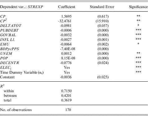
The results of the selected panel model are presented in Table 2.

Table 2

Results of the selected fixed effects panel model for the EU15.

Legend: Standard errors in parenthesis using Huber/White/sandwich estimator. ***, **, * refer to the significance at 1%, 5% and 10% respectively.

Source: own calculations.

The estimated model, explaining the dynamics of structural expenditures, with fixed effects included, has proven appropriate and highly significant; its explanatory power is very high. The model explains 71% of the variance in structural expenditure for the sample of EU Member States; at the same time, the signs of the regression coefficients for all variables were consistent with the theoretical expectations and, as a rule, the coefficients were statistically significant.

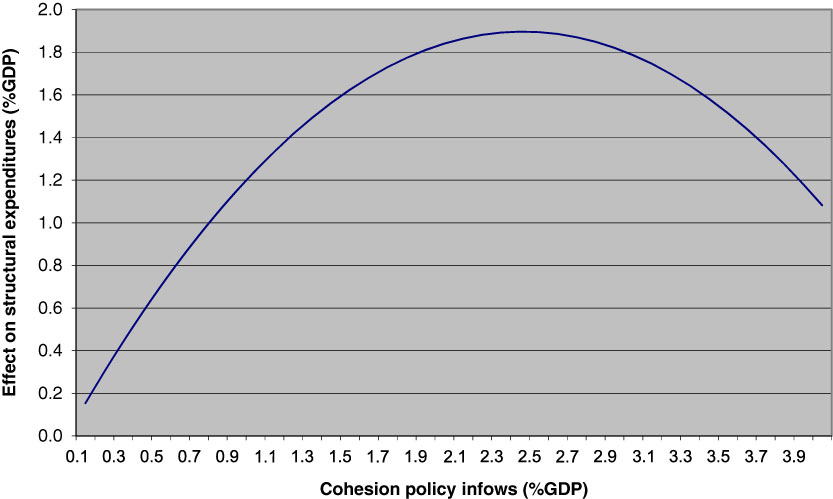
The effect of the inflows of cohesion policy funds (CP), a variable that is the most important for the model’s purpose, is statistically significant, positive, but non-linear. The partial effect of cohesion inflows on the amount of public structural expenditure is presented in Figure 1.

Figure 1

Partial average estimated effect of cohesion policy funds/inflows on the amount of structural expenditures. Source: own calculation.

Our results indicate that the cohesion policy funds/inflows represent additional public spending for economic purposes (including infrastructure), education and environment protection; hence, cohesion policy funds increase (rather than replace) the public structural expenditure in recipient countries. In the case of moderate inflows (up to approximately 1.75% of GDP), the additionality of funds is estimated on average to be complete. With minor inflows, the model even shows that the extent of structural expenditures is not only increased by the entire inflow of cohesion funds, but also by the required sum of own co-financing, which represents an additional leverage for cohesion policy funds. In the case of a more considerable inflow of cohesion funds (between approximately 1.75 and 2.33% of GDP p.a.), a minor rate of substitution was observed, in the range of up to 20% of total cohesion fund inflows. It then follows that at least 80% of the inflows represents a net increase in the amount of structural expenditure in the recipient countries. With inflows greater than 2.33% of GDP annually, the data show a more considerable rate of substitution or crowding out of domestic public structural expenditure. For example, if cohesion funds inflows would amount to 3% of GDP, the increase in structural expenditure would, according to the model, only reach 60%. That said, inflows of over 2.33% were historically granted only exceptionally, which means that cohesion funds in almost their entirety increased the amount of public structural expenditure, thus introducing an additional development incentive derived from public funds.

4.1 Robustness Analysis

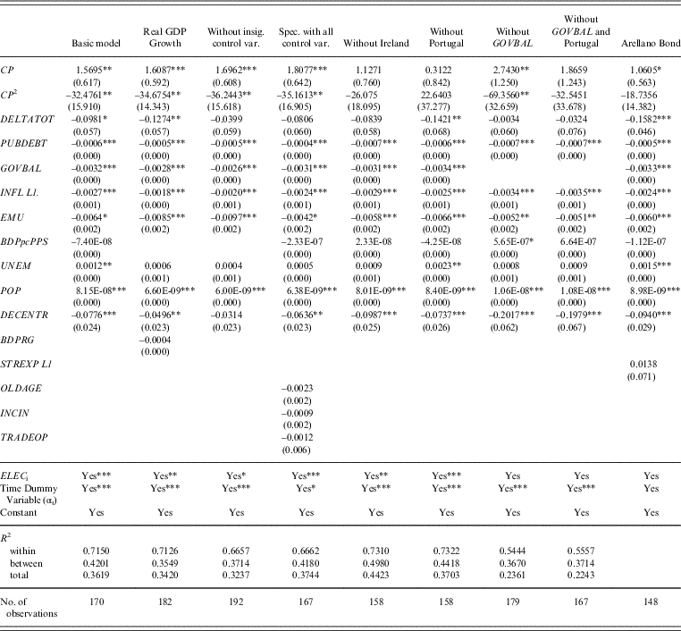
In order to test the robustness of the estimated results in the model above, a series of alternative specifications were conducted, confirming the findings of our original model. The unobserved, fixed effects are statistically significant and, as a result, the model of random effects is not appropriate, or rather, will not yield unbiased estimates; this was also confirmed by the Hausman test. The possibility of the effect with a time lag was also checked for all variables; however, this only proved appropriate in the case of changes in the rate of inflation. Logarithmic values as well as non-linear relationships were also tested.

Alternative model specifications also included a test for the validity of the so-called theory of incremental public expenditure growth,Reference Wildavsky ⁴⁴ which states that the most important determinant of the amount and composition of public expenditure is its composition in the previous year. The Arellano-Bond model was used for a dynamic specification of the model (see last column of Table 3), estimated by a generalized method of moments and using a lagged dependent variable and first differences of other explanatory variables. According to the Sargan test, the model specification is valid and the possibility of second-order autocorrelation is denied (which is a precondition for the use of the model); however, the lagged dependent variable proves not to be statistically significant, which fails to confirm the theory of incremental public spending growth and simultaneously confirms, or validates, the static specification of the model.

Table 3

Robustness analysis of the estimated model (various specifications and data samples; dependent variable is the amount of structural expenditure - percentage of GDP).

Legend: Standard errors in parenthesis using Huber/White/sandwich estimator. ***, **, * refer to the significance at 1%, 5% and 10% respectively.

Source: own calculations.

In addition to the key variables presented above, some additional or alternative variables were tested, which are relevant from the theoretical perspective, but failed to prove statistically significant. Hence, as an alternative specification for gross domestic product per capita, real growth of the gross domestic product (BDPRG, see second column of Table 3) was tested. In this case, too, the estimated relationship is negative, which could support the notion that in times of economic growth, governments are either seeking to re-structure public finance to a greater extent or trying to implement counter-cyclical measures; in any case, the effect is statistically not significant. In addition, virtually all other parameters remained robust and significant. The theoretically indicated effect of a country’s openness to trade was also tested, as well as the effect of income inequality and the importance of population age structure for the dynamics of structural expenditures. As can be seen from the fourth column of Table 3, all were proven statistically non-significant and without substantial effect on the value and significance of other parameters in the model, while the effect of cohesion inflows on structural expenditure is even slightly greater with this specification.

The results of the model have also been proven to be robust to the exclusion, or omission, of the non-significant variable (BDPpcPPS, i.e. GDP per capita in purchasing power standards) from the basic model, which can be seen from column three in Table 3. Similar to the previous case, the coefficients on the effect of the cohesion inflows on structural expenditure increased somewhat. The variable was kept in the basic model due to the control power of the GDP per capita.

Robustness in relation to the exclusion of individual countries was also tested. The results have proven robust to the exclusion of all countries except for Ireland and Portugal – which is not surprising. In addition to Greece, whose weight within the model is diminished because of the restricted time series of available data on government balance, these are the only two Member States that have received extensive inflows of cohesion funds. Their decisive effect on the significance of regression coefficients for cohesion policy was thus expected. Nevertheless, we also tested what happens if the variable of the government balance is also omitted; in this case, Greece, too, affects the results over the entire span of 12 years. The signs and significance of regression coefficients remained similar to those of the basic specification. The most obvious change was a somewhat more considerable increase in the coefficients for cohesion fund inflows. If, in addition to the previously eliminated variable, Portugal is also eliminated from this specification, the estimated effect of cohesion funds is again within the range of the values yielded by the basic model specification.

The robustness tests presented above have proven that the model is reliable; that the magnitude of the estimated regression coefficients does deviate from one specification to another, but these deviations generally do not affect their significance; and, above all, that these deviations remain reasonably moderate and do not affect the conclusions and findings yielded by the model. Finally, the estimated value of the effect of cohesion funds on the scope and amount of structural expenditures in the selected model is the mean value in the span of various alternative specifications, which additionally increases the reliability of the results.

5. Conclusion and Implications for Cohesion Policy

Whether the cohesion policy contributes to convergence, higher growth for targeted areas, creates jobs, and strengthens competitiveness, remains, at least from the scientific perspective, an open question. The differences in the assessment of cohesion policy’s effectiveness can be explained – to a considerable extent, though not entirely – by the methodological approaches employed. In principle the ‘econometric’ or ‘testing approach’ would seem to be the most appropriate as it directly measures the effect of the used resources; it, too however, faces methodological limitations.

We would argue that there are three main arguments for the problematic nature of direct testing of the macroeconomic effectiveness of cohesion policy resources. First, given the complexity of factors that influence economic growth, the effect of the cohesion funds is (too) minute to allow for its clear identification (Ref. 5, p. 129). Second, regarding its content, cohesion policy is highly heterogeneous both in terms of the purposes and in terms of extremely varied ‘initial conditions’ addressed and dealt with in different target areas. Hence, a ‘simple’ determination of average macro effect seems rather inappropriate in the case of such diverse contexts. Third, the available data, including that for cohesion policy expenditure, do not allow us, at least at this stage, to specify models detailed enough to capture causal relationships between cohesion policy and growth (or convergence). A related problem is a lagged effect of different investments, which could even theoretically be expected only in the long term, making it an almost insurmountable challenge for the testing approach.Reference Begg ⁶

This drove us to pursue a different course in this paper: to evaluate the macroeconomic effects of the cohesion policy in an indirect manner. The approach of this paper hence rests on the following logic. Cohesion policy expenditures represent a part of the broader package of public economic development policies. If it is true that, on average, government spending on the provision of public goods, particularly infrastructure and education, promotes economic growth, and considering the fact that cohesion funds are commonly allocated according to the institutional practice of the given region or country, then it can be concluded that the impact of cohesion funds will be comparable to the macroeconomic impact of general public spending on the above mentioned public goods. The existing empirical evidence does indeed assess this relationship to be predominantly positive.

Thus, the fundamental question we have posed was no longer what kind of impact cohesion funds bring directly to the economy, but rather to what extent they increase the amount of public spending, allocated for promoting development in target areas. This, so-called additionality of cohesion funds, is the necessary condition for any positive net effects to occur in the recipient country or region, while the actual effect of each particular investment will depend on: (a) micro-efficiency of the expenditures and (b) the impact of public on private investment. The question of micro-efficiency has been studied in depth in other studies,Reference Wostner ⁴⁵ while the work on the second question even points to additional crowding-in as opposed to the crowding-out effect.Reference de la Fuente ^{12 ,} Reference Afonso and Alegre ¹⁶

Based on an econometric model we have found that inflows from cohesion funds actually result in additional public expenditure for economic purposes (including infrastructure), education, and environment protection and that, hence, the cohesion policy funds tend to increase the net amount of public structural/development expenditure in recipient countries. The relationship has the shape of a quadratic function. With smaller inflows cohesion funds tend to set in motion additional leverage through the increase in structural expenditure due to co-financing requirements. Crowding out of national public spending can only be observed with higher inflows. Still, this negative effect only occurs with relatively high inflows. Hence, cohesion funds can be positively identified as net additional motivation for development, fuelled by public funding throughout the predominant part of the actual amounts of inflows. The results are robust to alternative specifications.

Our results seem to indicate that cohesion policy fulfils its fundamental mission of increasing public development investments in target areas. Given the restrictions with regard to the methodology and data availability, it would, nevertheless, be reasonable to devote additional attention to defining more specific indicators that would be consistent with the particular purpose for which the funds are granted; however, due to data restrictions this would only be possible at lower geographic levels (e.g. individual Member State, or preferably regions). For the same reason, experimental and quasi-experimental methods seem also to be a promising way forward.