1. Introduction
Is a country with weaker environmental standards capable of creating comparative advantage in the production of polluting products? Can it become a pollution haven? The Pollution Haven Hypothesis (PHH) answers these questions in the affirmative. However, several theoretical as well as empirical models of PHH give mixed results.
The purpose of our paper is to develop a sufficient condition under which the PHH is valid. We develop a 3 × 3 model with three goods and three inputs.Footnote 1 The input used to reduce environmental pollution, i.e. for abatement, is treated as a pure intermediate good.
Several theoretical models, such as Copeland and Taylor (Reference Copeland and Taylor1994, Reference Copeland and Taylor1997), prove that higher pollution taxes can reduce a country's comparative advantage in the polluting industry. Then, Chua (Reference Chua2003) shows how higher environmental taxes may not increase a country's comparative advantage in the dirty industry. By developing a counter example, Das and Das (Reference Das and Das2007) show that the PHH may not be valid in a 2 × 2 model with command and control (CAC) programs of regulation.Footnote 2 Copeland and Taylor (Reference Copeland and Taylor1995), Rauscher (Reference Rauscher1997), and McAusland (Reference McAusland2003) arrive at similar conclusions when the pollution in question is a by-product of consumption rather than production of dirty goods. Moreover, the empirical evidence on the PHH is inconclusive (Tobey, Reference Tobey1990; Liddle, Reference Liddle2001; Copeland and Taylor, Reference Copeland and Taylor2004), since besides the environmental standards, other factors like factor endowments also influence the pattern of trade and specialization.Footnote 3
The existing literature emphasizes economic incentives such as pollution taxes or tradable permits imposed by the regulator to reduce environmental pollution. However, several countries predominantly apply policies that set caps on allowable discharges of pollutants into the environment. Theoretical models such as Fullerton and Heutel (Reference Fullerton and Heutel2007) clearly recognize the effect of emission caps on factor prices in a general equilibrium setting. Therefore, our paper focuses entirely on the effect of command and control programs of regulation on the structure of production, distribution of income, and the patterns of trade in a standard neo-classical general equilibrium model.
Currently, the trade and environment literature is caught in a dilemma. If abatement is an input along with labor and capital, then, with one exportable and one importable good, the model turns into a 2 × 3 model and the standard trade theorems may not hold (Chua, Reference Chua2003). But the failure of standard trade theorems has nothing to do with the environment because these theorems may not hold in any 2 × 3 model. Casas (Reference Casas1972) is the first to develop a model of trade with pure intermediate goods. Copeland (Reference Copeland2005) treats inputs used for abatement as a pure intermediate good produced by labor. The intermediate-goods industry is monopolistically competitive and the final goods markets are perfectly competitive. The problem of unequal number of factors and goods does not arise in Copeland (Reference Copeland2005) since his model of emission taxes does not look into either the pattern of trade or comparative advantage. We suggest a way out of the trade–environment predicament by developing a 3 × 3 model where the environmental input is a pure intermediate good.
In this paper, we see that the PHH is valid only when the environmental policy is distribution neutral. Even with neutral abatement policies, a country can become a pollution haven only if it lowers emission caps in all industries. We use a dynamic panel model to test the distribution neutrality of US environmental policies. Our results indicate that the US environmental policies are consistent with distribution neutrality. We conclude that the US can become a pollution haven only if it lowers abatement standards in all industries.
We now plot a course for the rest of the paper. Section 2 introduces the 3 × 3 model where the abatement input is a pure intermediate good. Section 3 discusses the concept of distribution neutrality and tests whether US environmental policies are consistent with distribution neutrality. Section 4 concludes.
2. The theoretical model
We re-examine the standard neoclassical model with emphasis on abatement. In our model, X 1 and X 2 are the output levels of two final goods industries and A is the output of an intermediate-goods industry. Labor (L), capital (K), and the abatement input (A) produce X 1 and X 2. The non-tradable abatement input is produced by labor and capital. For production and achievement of a certain level of environmental standard, industry-1 needs L 1 units of labor, K 1 units of capital, and A 1 units of the abatement input; industry-2 needs L 2 units of labor, K 2 units of capital, and A 2 units of the abatement input; the intermediate-goods industry needs LA units of labor and KA units of capital.
We let C ij be the unit factor requirement for the ith input in the output of the jth industry (i = L, K, A; j = 1, 2, A). Thus, the unit factor requirements in industry-1 are, C L1 ≡ L 1/X 1, C K1 ≡ K 1/X 1, and C A1 ≡ A 1/X 1. In industry-2 these are, C L2 ≡ L 2/X 2, C K2 ≡ K 2/X 2, and C A2 ≡ A 2/X 2. For the intermediate-goods industry, C LA ≡ L A/A and C KA ≡ K A/A, where A 1 + A 2 = A. Our 3 × 3 model has eight input−output coefficients because we assume that no abatement input is needed to produce the abatement input, i.e. C AA = 0.
The total supply of labor in this economy is L = L 1 + L 2 + LA, total supply of capital is K = K 1 + K 2 + KA, and that of the intermediate good is A = A 1 + A 2. The following set of equilibrium conditions, (1)–(3), ensures full employment of labor, capital, and the abatement input.



The abatement coefficients, CA 1 and CA 2, are fixed as their values are determined by the environmental policy. When the environmental standard becomes more stringent, industries increase their abatement. The values of CA 1 and CA 2 increase under stricter environmental standards. Remaining input–output coefficients depend on the wage rate (w), rental rate (r), and the price of the abatement input (PA). In (4)–(6), all industries are perfectly competitive and long-run equilibrium is achieved when price equals average cost.



Given final-goods prices P 1 and P 2, and the values of CA 1 and CA 2, these six equations (1)–(6), can be solved for X 1, X 2, A, w, r, and PA. The prices of final goods in autarky equilibrium can be determined by bringing in the demand functions, while the price of the non-traded abatement input is determined along with the prices of primary inputs, labor, and capital.
This pure intermediate-goods model consisting of six equations can be reduced to a model of four equations. We eliminate A in equations (1) and (2) by using equation (3) and eliminate PA in equations (4) and (5) by using equation (6). Thus, we obtain the following equations (7)–(10)




where




Following the traditional pure intermediate-goods model of Casas (Reference Casas1972), we distinguish between gross and net unit factor requirements. In our model, for i = L, K and j = 1, 2; Rij are the gross unit factor requirements and C ij are the net unit factor requirements. Like Casas (Reference Casas1972), we define the factor intensity of a good in terms of Rij. Good 2 is capital intensive and good 1 is labor intensive if RK 2/RL 2 > RK 1/RL 1. A major difference between the traditional model and our model is, in the former, CA 1 and CA 2 are determined by a cost minimization process whereas, in our model, policy determines them.
Two factors can influence the gross coefficients RLj and RKj, (i) factor substitution in response to a change in ω ≡ w/r and (ii) policy induced changes in abatement requirements per unit of output, CA 1 and CA 2. A constant return to scale characterizes the technology in the two final-goods industries and the intermediate-goods industry. All final-goods industries minimize the average cost of production, ACj = wCLj + rCKj(j = 1, 2, A). The abatement input is non-traded and its price, PA, is determined in a competitive market. All industries take w, r, and PA as given. Policy determines CAj and therefore abatement cost is not a part of the cost minimization process. The shares of labor and capital in total production cost are SLj ≡ wCLj/ACj and SKj ≡ rCKj/ACj, where SLj + SKj = 1. An asterisk (*) represents any variable's total change measured by total derivatives. For instance, ω* = dω/ω. The cost minimization condition wdCLj + rdCKj = 0 is re-written as SLj(CLj)* + SKj(CKj)* = 0. Using the definition of the elasticity of substitution between K and L, (σj > 0; j = 1,2,A) we get (CKj)*−(CLj)* = σjω*. Solving for all C ij, (i = L, K), we get (12) and (13)

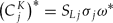
In the jth industry, (j = 1, 2), the proportions of labor used in production and abatement per unit of output are ξLj ≡ CLj/RLj and ξLAj ≡ CLACAj/RLj, such that ξLj + ξLAj = 1. Totally differentiating the labor coefficients in (11a) and (11b), we get RLj* = ξLjCLj* + ξLAjCLA*. Similarly, in the jth industry, (j = 1,2), the proportions of capital used in production and abatement per unit of output are ξKj ≡ CKj/RKj and ξKAj ≡ CKACAj/RKj, where ξKj + ξKAj = 1. We totally differentiate the capital coefficients in (11c) and (11d), and get RKj* = ξKjCKj* + ξKAjCKA*. To obtain (14) and (15), we use the solutions of C ij in (12) and (13) (i = L,K; j = 1,2,A)


2.1 Effect of environmental policy on factor markets
The shares of labor, capital, and abatement costs in the value added by the jth industry (j = 1, 2) are θLj ≡ wRLj/Pj, θKj ≡ rRKj/Pj, and θAj ≡ PACAj/Pj. We note that θLj + θKj = 1, as the cost of intermediate input is not included in value added to avoid double counting. We define |θ| ≡ θL 1θK2−θL2θK1. Therefore, |θ| and (RK 2/RL 2−RK 1/RL 1) have the same sign. If industry-2 is capital intensive and industry-1 is labor intensive, then |θ| is positive. The sign of |θ| is negative if industry-2 is labor intensive and industry-1 is capital intensive. Totally differentiating equations (9) and (10), we get


Solving (16) and (17) for w* and r*, we get


Defining ω = w/r and subtracting (19) from (18), we get

2.2 Environmental policy and distribution neutrality
Under stricter environmental policies, both final-goods industries increase their abatement, i.e. (CA 1)* > 0 and (CA 2)* > 0. We now derive a condition under which changes in environmental policy do not affect the distribution of income. In (20), the direct effect of environmental policy on income distribution is (θA2(CA 2)*−θA1(CA 1)*)/|θ|. The abatement policy is distribution neutral under the following condition

2.3 Production and trade under distribution neutral environmental policy
Under (21), environmental policy has no impact on the distribution of income. This becomes apparent if we apply (21) in (20) to get

where, P* = P*2−P*1.
For j = 1,2, the proportions of labor and capital directly and indirectly used in producing the jth good are λLj ≡ RLjXj/L and λKj ≡ RKjXj/K. The proportions of labor and capital used in producing the abatement input for the jth good are λLAj = CLACAjXj/L and λKAj = CKACAjXj/K. Any changes in the abatement requirements will alter the structure of production in a rather complex way. To see this, we totally differentiate (7) and (8)


We note the same accounting balance, λL1 + λL2 = λK1 + λK2 = 1. We define |λ| ≡ λL1λK2−λL2λK1 = λL1−λK1 = λK2−λL2. Therefore, |λ|, |θ| and (RK 2/RL 2−RK 1/RL 1) have the same sign. If industry-2 is capital intensive and industry-1 is labor intensive, then |λ| is positive. The sign of |λ| is negative if industry-2 is labor intensive and industry-1 is capital intensive. Using (22), which is valid only under the distribution neutrality assumption and definitions of Rij(i = L,K; j = 1,2), we obtain the following relationships
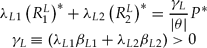
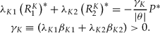
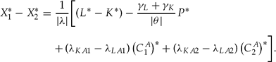
Subtracting (24) from (23), using the properties of |λ| and the relationships (25) and (26), which are valid only under the distribution neutrality assumption, we get
To close the model we introduce a homothetic utility function. The ratio in which goods are demanded (D 1/D 2) depends only on the relative price (P 2/P 1) and the elasticity of substitution, σD > 0. As P ≡ P 2/P 1 rises, the consumers substitute in favor of the first good, which raises D 1/D 2. Therefore

We define k* ≡ K* – L* and σS = (γL + γK)/|θ|. In autarky equilibrium, X 1*−X 2* = D 1*−D 2*. From this equilibrium condition, (27) and (28), we obtain the autarchy terms of trade

Proposition 1If abatement input is regarded as a pure intermediate good used in the final-goods industries and if factor intensities are defined in terms of gross input–output coefficients, then for any given set of environmental standards that are distribution neutral, all neo-classical trade theorems are valid, namely Stolper–Samuelson, Rybczynski and Heckscher–Ohlin theorems.
Under the distribution neutrality assumption, all neo-classical trade theorems are valid. The Stolper–Samuelson theorem follows from (22), which shows a unique relationship between factor and product prices. Equation (27) illustrates the validity of the Rybczynski theorem. At constant terms of trade (P* = 0) and environmental standard (CA 1* = CA 2* = 0), an increase in the supply of labor (L* > 0) raises the relative output of the labor-intensive good (X 1* – X 2* > 0 if |λ| > 0); while an increase in the supply of capital (K* > 0) increases the relative output of the capital-intensive good (X 1* – X 2* > 0 if |λ|<0). Equation (29) shows that the Heckscher–Ohlin theorem would determine the trade pattern between countries with small differences in environmental policy. With small or negligible differences in environmental policies (CA 1* = CA 2* = 0), a labor-abundant country has comparative advantage in the labor-intensive good, whereas a capital-abundant country has comparative advantage in the capital-intensive good.
2.4 Uniform comparative advantage
We find a relationship between variations in the environmental standards set for the two final-goods industries. The distribution neutrality assumption is re-stated as

We define the market share of the first industry θ1 = P 1X 1/(P 1X 1 + P 2X 2), use the definitions of λLAj and λKAj, apply the relationship between (CA 1)* and (CA 2)* from (21a), and get


Proposition 2Countries cannot change their position of comparative advantage by following a discriminatory environmental policy, setting liberal standards for one sector and stringent standards for the other. The effect of the environmental standard on comparative advantage is uniform for all industries.
Equation (21a) shows that the signs of (CA 1)* and (CA 2)* are the same. Therefore, in equation (31), the effect of environmental policy on autarchy terms of trade is uniform. The abatement standards cannot be changed in industry-1 without changing them in industry-2.
2.5 PHH and distribution neutral abatement policy
According to proposition 1, the neo-classical trade theorems are valid if environmental policies are distribution neutral. The Heckscher–Ohlin theorem determines the pattern of trade between a labor-abundant country and a capital-abundant country with small differences in environmental policy. Without the assumption in (21), change in the abatement standard changes the wage/rental ratio in (20), which changes the autarky terms of trade in (29). More specifically, if (20) is used in place of (22), then the computations in (14), (15), (25), and (26) are complicated and the validity of all trade theorems is ambiguous.
Can countries manipulate their environmental standards to improve their comparative advantage? According to proposition 2, the effect of abatement standards on comparative advantage is uniform in all industries. A country may however follow a policy of changing abatement requirements for the two final-goods industries in opposite directions (sign of (CA 1)* = –sign of (CA 2)*). However, such a policy violates the assumption of distribution neutrality in (21). The effect of such policies on the pattern of trade is indeterminate.
We now focus on equation (31), where the effect of a distribution neutral abatement policy on comparative advantage depends on the sign of (λKA 1−λLA 1), which is positive if the proportion of capital is more than the proportion of labor used in producing the abatement input for good 1. We use the definitions of λKAj and λLAj (j = 1,2) and note (λKAj−λLAj) = CAjXj[(CKA/K)−(CLA/L)]. Therefore, the sign of (λKA1−λLA1) is the same as the sign of (λKA2−λLA2). Since abatement of pollution is generally capital intensive, we expect (λKA1−λLA1) to have a positive sign. We define g ≡–1/|λ|(σD + σS) and f ≡ [1/|λ|(σD + σS)](λKA1−λLA1) (1/θ1). In order to see the effect of environmental policy on comparative advantage, we solve the differential equations in (31), to get

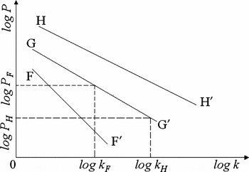
Figure 1 illustrates the relationship between the autarky price and the factor endowment ratio. The line GG’ is common for two countries, H (home country) and F (foreign country), with identical environmental policies. The capital abundant home country (kH > kF) has comparative advantage in the capital-intensive second good (|λ| > 0). If the home country has a stricter standard for both industries and the foreign country reduces it in all industries, their graphs are respectively denoted by HH′ and FF′. The home country's comparative advantage in the capital-intensive good suffers and the foreign country can gain comparative advantage in the capital-intensive good by lowering their environmental standards. Our analysis so far assumes the environmental policy is distribution neutral. In other words, the home country raises the pollution abatement standard for both industries and the foreign country reduces it for all industries. Proposition 3 summarizes this argument.
Environmental standard and comparative advantage

Proposition 3It is doubtful that a country can become a pollution haven by following discriminatory environmental policies where abatement standards vary from one industry to another. However, a country can become a pollution haven by setting uniformly regressive abatement standards in all industries.
According to the PHH, weak environmental standards improve a country's comparative advantage in the polluting industry. Pollution havens are created in a country that imposes lenient abatement standards for a polluting industry, while another country enforces stringent abatement standards for the same industry. Proposition 3, however, presents a more damaging scenario. In order to create a pollution haven, a country has to raise the level of pollution in all sectors. In our model, raising the abatement standard selectively in some sectors, violates the distribution neutrality assumption and may not give it a clear-cut advantage.
3. Testing the distribution neutrality assumption
3.1 Interpretation of the distribution neutrality assumption
The concept of distribution neutral abatement policy is inspired from the US Clean Air Act (amended 1990). Title I of the amended 1990 Act makes a clear distinction between ‘existing’ and ‘new’ sources of air pollution and imposes lenient standards on the former. Part A, Section 112 talks about national emission standards for hazardous air pollution. It states:
The maximum degree of reduction in emissions that is deemed achievable for new sources in a category or subcategory shall not be less stringent than the emission control that is achieved in practice by the best controlled similar source, as determined by the Administrator. Emission standards promulgated under this subsection for existing sources in a category or subcategory may be less stringent than standards for new sources in the same category or subcategory but shall not be less stringent, and may be more stringent than- (A) the average emission limitation achieved by the best performing 12 percent of the existing sources . . .
The condition for distribution neutrality stated in equation (21) has the following implications:

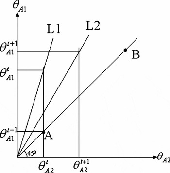
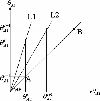
Figure 2 provides an interpretation of the distribution neutrality condition. Point A on a 45° line illustrates the initial situation of two industries with identical shares of abatement cost in value added. Both industries are required to move to a point B on the 45° line when the abatement standard becomes more stringent. If the first industry complies at time t and the second industry does not, both industries move to a point on line L1. Equation (33) implies, in the next period that they will move to a point on line L2. Since L2 is closer to the 45° line, therefore, as shown in the diagram,  < 1. We test this implication of the distribution neutrality assumption with a dynamic panel model.
Distribution neutrality
3.2 Data
We use data on pollution abatement costs from the US Census Bureau's Pollution Abatement Costs and Expenditures (PACE) survey. These data are published in Current Industrial Reports: Pollution Abatement Costs and Expenditures, MA-200. Levinson and Taylor (Reference Levinson and Taylor2008) discuss several challenges researchers may face while using this dataset. Taking their suggestions, we use only the PACE operating cost data as a proxy for the cost of abatement. In 1987, several 3-digit SIC codes were substantially changed making post-1987 data incomparable with pre-1987 data. In addition, the PACE survey was not conducted in 1987, resulting in missing data problems in the entire time series. To avoid these problems we focus on the operating cost data for 19 industries classified under the 2-digit SIC codes for the years 1977 to 1986. For the value added and total cost of production data, we refer to the Annual Survey of Manufactures (AS)-1, published by the US Census Bureau, Department of Commerce.
3.3 The econometric model and results
To test the distribution neutrality assumption, we estimate the following dynamic panel model
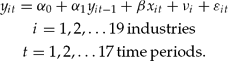
The ith industry's share of abatement cost in value added at time t is represented by yit. We consider a model where past realizations of an industry's share of abatement cost in value added affects its current levels. We see from (33) that the distribution neutral abatement policy implies α 1<1. In (33) we assume that prices do not change between the time periods t and t + 1. Therefore, to capture the effect of price changes, we include the explanatory variable xit, the ith industry's share of abatement cost in total cost.Footnote 4 In (34), α0, α1, and β are parameters, νi are random effects that are independently and identically distributed (i.i.d) over the panels with variance σ2ν, and ɛit are i.i.d over the whole sample with variance σ2ϵ.
As Nickell (Reference Nickell1981) shows, the lagged dependent variable is correlated with the error term. As a result, y it−1 is endogenous and the OLS estimate of the co-efficient of the lagged dependent variable is inconsistent. The first difference transformation of (34) removes vi and the constant term

In (35), the differenced lagged dependent variable and the disturbance process are still correlated. Anderson and Hsiao (Reference Anderson and Hsiao1982) construct instruments (IV) for Δyit– 1 from the differences or lagged levels of the second and third lags of y. The IV approach of Anderson–Hsiao does not exploit all the information available in the sample. Arellano and Bond (Reference Arellano and Bond1991) derive a generalized method of moments estimator for α 1, which is more efficient than the IV estimates. Their method assumes that there is no second-order autocorrelation in the first differenced idiosyncratic errors.
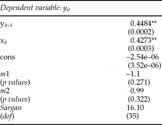
In table 1, we state the Arellano–Bond difference GMM estimates. From the dynamic panel model, the two-step Arellano–Bond GMM estimate of α 1 is significantly less than one at the 1 per cent level. We also fail to reject the null hypothesis of no autocorrelation of order 1 or order 2 in the first differenced residuals. The Sargan (Reference Sargan1958) test of over-identifying restrictions does not reject the validity of instruments for the GMM model.
Arellano bond difference GMM estimates (all variables in first differences)
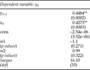
Notes: 1. m1 and m2 are tests for first-order and second-order serial correlation in the first differenced residuals, asymptotically distributed as N(0,1), under the null of no serial correlation.
2. Sargan is a test of over-identifying restrictions, asymptotically distributed as χ 2 under the null of instrument validity, with degrees of freedom and p values reported in parentheses.
3. ** indicates significance at 1% level and * indicates significance at 5% level.
Alonso-Borrego and Arellano (Reference Alonso-Borrego and Arellano1999) find large finite sample bias and poor precision in GMM estimates, particularly when the autoregressive parameter is moderately large and the number of time series observations is moderately small. Blundell and Bond (Reference Blundell and Bond1998) consider alternative estimators, which improve the properties of standard first-differenced GMM estimators. They propose the use of an extended linear GMM estimator that uses lagged differences of yit as instruments for equations in levels, in addition to lagged levels of yit as instruments for equations in first differences. Extended GMM estimates provide dramatic efficiency gains.
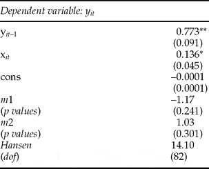
Table 2 gives us the Blundell–Bond extended GMM estimates. These are the system GMM estimates that are based on three moment conditions. From the dynamic panel model, the Blundell–Bond system GMM estimate of α 1 is significantly less than one at the 1 per cent level. We use the finite-sample correction to the two-step covariance matrix derived by Windmeijer (Reference Windmeijer2005) to get robust results. Again, we fail to reject the null hypothesis of no first- or second-order serial correlation in the first differenced residuals. The extended set of moment restrictions is not rejected by the Hansen (Reference Hansen1982) test of over-identifying restrictions.
Blundell bond system GMM estimates
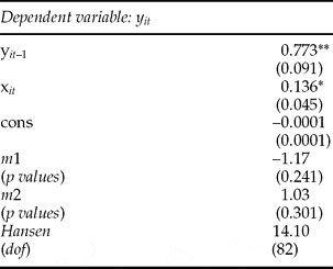
Notes: 1. m1 and m2 are tests for first-order and second-order serial correlation in the first differenced residuals, asymptotically distributed as N(0,1), under the null of no serial correlation.
2. Hansen is a test of over-identifying restrictions, asymptotically distributed as χ 2 under the null of instrument validity, with degrees of freedom and p values reported in parentheses.
3. ** indicates significance at 1% level and * indicates significance at 5% level.
The first differenced Arellano–Bond GMM estimate, as well the Blundell–Bond system GMM estimate of α 1 are significantly less than one. The dynamic panel data results indicate that the US environmental policy is consistent with distribution neutrality. According to the theoretical model of the paper, with distribution neutrality, to create a pollution haven, the US will have to lower environmental standards in all industries.
3.4 A test for unit roots in dynamic panels
To test for the presence of unit root, we use Levin et al. (Reference Levin, Lin and Chu2002) to test for dynamic panels with small N and T. Their test determines whether the stochastic process {yit} is integrated for each individual i in the panel for i = 1, 2, . . ., N and t = 1,2, . . ., T. The panel test procedure evaluates the null hypothesis that each individual time series contains a unit root against the alternate hypothesis that each time series is stationary.Footnote 5 We calculate the test statistic t* =–1.94075 (P > |t| = 0.0261) and reject the null hypothesis that each individual time series contains a unit root.
4. Conclusions
Our paper concentrates on the impact of environmental policies on the pattern of specialization and the distribution of income. If abatement is modeled as a pure intermediate good, income distribution deserves more importance than what the existing literature confers. The PHH states that countries with lower environmental compliance costs specialize in the production and export of products produced by polluting industries. It is also suggested that some nations actively seek foreign investment by becoming pollution havens. The theoretical model with 3 goods and 3 inputs, presented in this paper, provides an analytical framework for the PHH. We present a simple general equilibrium model of trade under CAC programs of environmental regulation, to highlight certain unanticipated consequences of governmental intervention. Regulation alters the wage/rental ratio, which has implications for factors used in production as well as abatement. Generally, the effect of abatement policy on the pattern of trade is indeterminate. The PHH as well as the neoclassical trade theorems are valid only when environmental policies are distribution neutral. Inspired by the US Clean Air Act, we test the validity of the distribution neutrality assumption by developing and estimating a dynamic panel model. We use abatement cost and manufacturing data published by the US Census Bureau and find that the US environmental policy is consistent with distribution neutrality. It is commonly believed that a country can selectively choose sectors to create a pollution haven. Our theoretical model suggests that this is unlikely to happen if abatement policy is distribution neutral. With distribution neutrality, to create pollution havens a country has to allow all industries to pollute more. Our results indicate that the US can become a pollution haven only if it lowers abatement standards in all industries, a policy with devastating consequences for the world environment. Are there other countries in the world where environmental policies are consistent with distribution neutrality? Do other countries create pollution havens by relaxing environmental standards in all industries? These questions need to be answered in future studies.