
 Kn





1. Introduction
Gas flows in the rarefied regime exhibit behaviour fundamentally different from that predicted by the classical continuum equations. As the characteristic length and time scales of a flow become comparable to the molecular mean free path and mean collision time, respectively, the assumptions underlying the Navier–Stokes–Fourier (NSF) description break down and non-equilibrium effects become significant (Sone Reference Sone2007; Roohi et al. Reference Roohi, Akhlaghi and Stefanov2025). In such cases, intermolecular collisions, molecule–surface interactions and ballistic transport play essential roles, leading to transport phenomena that cannot be captured by continuum theory alone. Kinetic gas theory is then of central importance for the analysis of micro- and nanoscale systems, vacuum technologies and low-density aerodynamic environments.
Among the many non-equilibrium phenomena that arise at non-continuum conditions, thermally induced flows are of particular interest. These motions are driven by temperature non-uniformities, even in the absence of externally imposed pressure gradients or moving boundaries (Sone Reference Sone2000; Akhlaghi et al. Reference Akhlaghi, Roohi and Stefanov2023; Roohi et al. Reference Roohi, Akhlaghi and Stefanov2025). Depending on the degree of gas rarefaction and the thermal configuration, several distinct mechanisms may become effective, including thermal creep (Sone Reference Sone1966; Ohwada et al. Reference Ohwada, Sone and Aoki1989; Han et al. Reference Han, Muntz, Alexeenko and Young2007), thermal stress (Rafieenasab et al. Reference Rafieenasab, Roohi and Teymourtash2020; Mousivand & Roohi Reference Mousivand and Roohi2022a ) and the occurrence of radiometric force loading (Taguchi & Aoki Reference Taguchi and Aoki2015; Shahabi et al. Reference Shahabi, Baier, Roohi and Hardt2017; Lotfian & Roohi Reference Lotfian and Roohi2019). In addition, thermal edge flows, where gas motion is induced by sharp temperature discontinuities along a surface, have been considered in detail (Sone & Yoshimoto Reference Sone and Yoshimoto1997; Aoki et al. Reference Aoki, Sone and Waniguchi1998, Reference Aoki, Takata, Aikawa and Golse2001; Taguchi & Aoki Reference Taguchi and Aoki2012; Rafieenasab et al. Reference Rafieenasab, Roohi and Manela2026). Such effects are inherently kinetic in origin and are absent from the NSF description in the continuum limit under uniform pressure and stationary wall conditions. Notably, thermally induced flows have attracted considerable attention over the years due to their fundamental importance and practical relevance in applications such as Knudsen pumps (Knudsen Reference Knudsen1909; Baier et al. Reference Baier, Hardt, Shahabi and Roohi2017), micro-Pirani gauges (Zhang et al. Reference Zhang, Tang, Yu and Jin2006) and other vacuum-based applications (Turnbull et al. Reference Turnbull, Barton, Riviere and Pasternak1962).
Within the context of thermally induced flows, the closed-cavity configuration with non-uniformly heated walls, commonly encountered in vacuum packaged devices (Cai Reference Cai2008), has been investigated. In such enclosures, temperature differences along the boundaries may generate internal circulatory motion. The resulting flow patterns, including complex vortical structures (Papadopoulos & Rosner Reference Papadopoulos and Rosner1995; Rana et al. Reference Rana, Torrilhon and Struchtrup2012; Vargas et al. Reference Vargas, Tatsios, Valougeorgis and Stefanov2014), are of considerable theoretical and practical interest. From a theoretical perspective, this configuration provides a canonical model problem for studying the interplay between ballistic molecular transport, intermolecular collisions and wall boundary conditions. From a practical perspective, understanding such thermally induced cavity flows is relevant to the thermal management and gas-dynamic behaviour of confined rarefied gases in various microsystems and low-pressure environments.
To analyse the problem, Taguchi & Tsuji (Reference Taguchi and Tsuji2020) studied the motion of a slightly rarefied gas induced by a discontinuous surface temperature, using the linearised Bhatnagar–Gross–Krook (BGK) kinetic model (Bhatnagar et al. Reference Bhatnagar, Gross and Krook1954). Focusing on the slip and transition regimes,Moghadam et al. (Reference Moghadam, Roohi and Esfahani2014) investigated a square cavity with heat-flux boundary conditions using the direct simulation Monte Carlo (DSMC) method. Papadopoulos & Rosner (Reference Papadopoulos and Rosner1995) and Hssikou et al. (Reference Hssikou, Baliti and Alaoui2019) examined the flow pattern in a square cavity, where two opposite walls were maintained at uniform hot and cold temperatures, and the remaining walls were subject to linear temperature variations. Zhang et al. (Reference Zhang, Yao, Fei, Ghalambaz and Wen2020) further considered the influence of gravity on the problem, and Vargas et al. (Reference Vargas, Tatsios, Valougeorgis and Stefanov2014) investigated the effects of cavity aspect ratio in a wide range of Knudsen numbers. Zhu et al. (Reference Zhu, Yang and Guo2017) extended this type of thermal configuration to a three-dimensional channel, through numerical analysis of the Shakhov kinetic model (Shakhov Reference Shakhov1968).
In a parallel set of works, a square cavity configuration with a uniformly heated bottom wall was considered. Liu et al. (Reference Liu, Wang, Wang, Zhang, Liao, Huang and Zhang2007) applied the DSMC method in the near-continuum regime, whereas Rana et al. (Reference Rana, Torrilhon and Struchtrup2012) considered the regularised 13-moment equations to describe the system behaviour in the continuum through early transition conditions. Cai (Reference Cai2008) provided an analytical solution in the free-molecular limit, together with numerical results in the near-continuum case. Mousivand & Roohi (Reference Mousivand and Roohi2022b ) analysed numerically a square cavity setup, where the top and bottom walls were kept at a uniform temperature and the side walls were maintained at a lower uniform temperature, revealing the characteristic vortical structure and its overall direction over a broad range of Knudsen numbers.
Considering the free-molecular limit of thermally driven flows about stationary bodies, the ballistic field has been previously analysed by Sone and coworkers (see, e.g., Sone (Reference Sone1984, Reference Sone1985, Reference Sone2000, Reference Sone2007, Reference Sone2009) and works cited therein). The solution presented indicates that the collisionless field may be obtained for a broad class of configurations, where the associated macroscopic gas state is invariably quiescent. These findings, however, describe the limiting ballistic state and do not describe the system behaviour at finite (even if large) Knudsen numbers.
Three gaps emerge from the body of work reviewed above. First, with the exception of the free-molecular analysis of Cai (Reference Cai2008) and the general free-molecular solutions by Sone (Reference Sone2000, Reference Sone2007), existing treatments rely almost exclusively on computationally intensive numerical simulation, predominantly the DSMC method, and therefore offer limited insight into the kinetic mechanism underlying the induced motion. Second, the available analytical work is concentrated in the slip and early transition regimes, where thermal creep and thermal stress dominate, whereas the opposite near-free-molecular limit remains comparatively unexplored. Third, the analyses that do reach high rarefaction are largely restricted to linearised kinetic models or to small wall-temperature differences, leaving the strongly nonlinear, finite-temperature-difference regime unexplored. Consequently, an analytical description of how weak intermolecular interactions modify the collisionless state and generate finite-Knudsen-number circulation remains lacking.
The present work addresses these gaps directly. Adopting the double-hot–double-cold cavity configuration of Mousivand & Roohi (Reference Mousivand and Roohi2022b ), we derive a near-free-molecular asymptotic solution for the full nonlinear hard-sphere (HS) Boltzmann collision operator, together with the BGK and Shakhov models. In contrast to earlier high-Knudsen-number analyses, these solutions hold for arbitrary cold-to-hot wall-temperature ratios, removing the linearisation and small-temperature-difference restrictions of previous linearised treatments (Taguchi & Tsuji Reference Taguchi and Tsuji2020). The analysis identifies the near-ballistic collisional mechanism by which even a small amount of intermolecular interactions generate thermally induced circulation. Specifically, wall-emitted molecular populations carry unequal trajectory-weighted momenta, so that the first collisional correction drives a net cold-to-hot slip whose amplitude grows as the Knudsen number decreases. In this respect, the present work complements the known free-molecular solutions by Sone (Reference Sone2007) and others, through the description of the finite-Knudsen-number correction that gives rise to thermally induced motion away from the collisionless limit. Combined with DSMC and particle-based solutions that span all Knudsen numbers, this yields a comprehensive description of the thermally induced flow over all rarefaction rates, including quantification of the location and magnitude of the flow-intensity maximum. In the continuum limit, the gas thermodynamic state is compared with a ‘pure conduction’ solution for the temperature. The quantitative differences between the HS, BGK and Shakhov descriptions are examined.
The work outline is as follows. The problem formulation is presented in § 2, followed by the derivation of the analytical free-molecular and the high-Knudsen-number asymptotic solutions in § 3. The continuum description is obtained in § 4, and the numerical schemes applied to analyse the problem at arbitrary rarefaction rates are described in § 5. Our results are presented in § 6, followed by a summary of our conclusions in § 7.
2. Formulation of the problem
2.1. Problem statement
Schematic of the problem. A square cavity of side length
 $L^*$
is filled with a perfect monatomic gas. The horizontal and vertical walls are maintained at temperatures
 $T_{h}^*$
and
 $T_{c}^*$
, respectively, where
 $T_{h}^*\gt T_{c}^*$
. Each wall is labelled a number, and the indicated angles
 $\theta _i$
(
 $i=1,\ldots ,4$
) correspond to the angles introduced in (3.11).

Figure 1. Long description
A schematic of a square cavity with side length L*. The cavity is filled with a perfect monatomic gas. The horizontal walls are maintained at temperature T_h, and the vertical walls are maintained at temperature T_c, where T_h is greater than T_c. Each wall is labeled with a number: the top wall is labeled 1, the bottom wall is labeled 2, the right wall is labeled 3, and the left wall is labeled 4. The angles θ1, θ2, θ3, and θ4 are indicated at the intersection of the dashed lines, which represent the directions of gas flow due to temperature differences. The x* and y* axes are shown at the center of the cavity, indicating the coordinate system used for analysis.
A schematic of the problem is shown in figure 1. We consider a perfect monatomic gas enclosed in a two-dimensional square cavity of side length
 $L^*$
(hereafter, asterisks denote dimensional quantities). The total gas mass contained in the cavity per unit length (in its spanwise direction) is
 $m^*_{\textit{tot}}$
. No external body forces, including gravity, act on the gas. The top and bottom cavity walls are maintained at a constant temperature
 $T_{h}^*$
, and are labelled as walls 1 and 3, respectively, and the left and right boundaries are fixed at temperature
 $T_{c}^*$
and labelled wall numbers 2 and 4, respectively. Without loss of generality, we assume
 $T_{h}^* \gt T_{c}^*$
. The origin of the
 $(x^*,y^*)$
coordinate system is located at the cavity centre point, and we seek to analyse the steady flow field generated in the cavity at arbitrary gas rarefaction rates.
In the framework of gas kinetic theory and the present two-dimensional steady-flow setup, the gas state is governed by the probability density function
 $f^* = f^*(x^*,y^*,\boldsymbol{\xi }^*)$
of finding a molecule at a position
 $\boldsymbol{r^*}=(x^*,y^*)$
with molecular velocity
 $\boldsymbol{\xi }^*$
. To analyse the velocity space, a cylindrical coordinate system is adopted, where
 $\boldsymbol{\xi }^* = (\xi _r^*,\theta _\xi ,\xi _z^*)$
. Here,
 $\xi _r^* \in [0,\infty )$
denotes the molecular speed in the plane of motion,
 $\theta _\xi$
marks the in-plane counterclockwise velocity direction and
 $\xi _z^* \in (-\infty ,\infty )$
is the velocity component normal to the cavity. To model gas–surface interactions between the gas particles and the solid walls, we apply the diffuse Maxwell boundary condition (Sone Reference Sone2007),
 \begin{equation} f^*({\boldsymbol{\widetilde {r}}_{i}^*},\boldsymbol{\xi }^*\boldsymbol{\cdot }\hat{\boldsymbol{n}}\gt 0)=\frac {\rho ^*_i(\boldsymbol{\widetilde {r}}_i^*)}{(\pi 2\mathcal{R}^*_gT^*_i)^{3/2}}\exp {\left [-\frac {{\xi ^*}^2}{2\mathcal{R}^*_gT^*_i}\right ]}, \end{equation}
stating that the reflected particles achieve thermal equilibrium with their reflecting boundaries. In (2.1),
 $\boldsymbol{\widetilde {r}}_i^*$
marks some point along the
 $i$
th wall
 $(i=1,\ldots ,4)$
,
 $\hat{\boldsymbol{n}}$
is a unit vector directed normal to the wall and into the gas domain and
 $\rho _i^*(\boldsymbol{\widetilde {r}}_i^*)$
are yet unknown functions associated with the mass flux of particles reflected from the
 $i$
th wall. In addition,
 $U_{{mp}_{i}}=(2\mathcal{R}_g^* T_i^*)^{1/2}$
denotes the most probable speed of gas particles at the
 $i$
th wall temperature, where
 $\mathcal{R}_g^*$
is the specific gas constant and
 $T_i^*$
is the temperature of the
 $i$
th wall. In line with figure 1, the temperatures of the walls are
 $T_{1}^*=T_{3}^* = T_{h}^*$
and
 $T_{2}^*=T_{4}^* = T_{c}^*$
.
To render the problem dimensionless, we scale the position by the cavity side length
 $L^*$
, the velocity by the
 $T_h^*$
-based wall temperature most probable molecular speed,
 $U_{{mp}_{h}}^*=(2\mathcal{R}^*_g T^*_{h})^{1/2}$
, and the temperature by
 $T^*_{h}$
. The density is normalised by the average density based on the total mass of the gas confined in the cavity,
 $\rho _0^*=m^*_{\textit{tot}}/L^{*2}$
, and the pressure is non-dimensionalised by
 $\rho _0^*\mathcal{R}^*_gT_h^*$
. The system non-dimensional description is then governed by the cold-to-hot wall temperature ratio and the gas mean Knudsen number,
 \begin{equation} R_T=T_c^*/T_h^* \quad \mathrm{and} \quad \textit{Kn} = \lambda ^*/L^*, \end{equation}
respectively, where
 $\lambda ^*$
denotes the mean free path of a gas molecule. Assuming an HS interaction gas model,
 $\lambda ^* = m^*/(\pi \sqrt {2}\rho _0^* d^{*2})$
, where
 $m^*$
and
 $d^*$
denote the mass and diameter of a gas particle, respectively (Sone Reference Sone2007). Substituting
 $\lambda ^*$
into (2.2), we obtain
 \begin{equation} \textit{Kn} = \frac {m^*}{\pi \sqrt {2}\rho ^*_0 d^{*2}L^*} \ . \end{equation}
The problem statement is completed by imposing a normalisation condition for the gas density
 $\rho$
, fixing the total gas mass in the cavity,
 \begin{equation} \int _{-1/2}^{1/2}\int _{-1/2}^{1/2}\rho (x,y)\,\mathrm{d}x\,\mathrm{d}y=1 . \end{equation}
In what follows, we introduce the kinetic models to be used to formulate the collision operator in the Boltzmann equation.
2.2. The model equations
Adopting the scaling introduced in § 2, and within the two-dimensional steady setup considered, the scaled velocity distribution function
 \begin{equation} f = \frac {(2\mathcal{R}_g^* T_{h}^*)^{3/2}}{\rho _0^*} f^* \end{equation}
is governed by the non-dimensional Boltzmann-type equation
 \begin{equation} \boldsymbol{\xi }\boldsymbol{\cdot }\boldsymbol{\nabla }\!f= \frac {1}{\textit{Kn}}\mathcal{J}(f), \end{equation}
where
 $\mathcal{J}(f)$
denotes the nonlinear integral collision operator, accounting for the effect of binary molecular collisions on the evolution of the distribution function. For HS gas, the corresponding scaled collision operator is given by (Kogan 1969).
 \begin{equation} \mathcal{J}_{\textit{HS}}(f) = \frac {1}{2\sqrt 2\pi }\int \left (f(\boldsymbol{r},\boldsymbol{\xi '})f(\boldsymbol{r},\boldsymbol{\xi '_1})-f(\boldsymbol{r},\boldsymbol{\xi })f(\boldsymbol{r},\boldsymbol{\xi _1})\right ) |\boldsymbol{g}\boldsymbol{\cdot }\hat {\boldsymbol{k}}|\,\mathrm{d}\varOmega \,\mathrm{d\boldsymbol{\xi _1}} , \end{equation}
where
 $\mathrm{d}\varOmega$
denotes the solid-angle element associated with its unit vector
 $\hat {\boldsymbol{k}}$
,
 $\boldsymbol{\xi }_1$
is the integration variable corresponding to the molecular velocity, and
 $\boldsymbol{g} = \boldsymbol{\xi }_1 - \boldsymbol{\xi }$
is the relative velocity between particles prior to collision. The post-collision molecular velocities are
 \begin{equation} \boldsymbol{\xi }' = \boldsymbol{\xi } + \hat{\boldsymbol{k}} (\hat{\boldsymbol{k}} \boldsymbol{\cdot }\boldsymbol{g}) \ \ \ \mathrm{and} \ \ \ \boldsymbol{\xi }_1' = \boldsymbol{\xi }_1 - \hat{\boldsymbol{k}} (\hat{\boldsymbol{k}} \boldsymbol{\cdot }\boldsymbol{g}). \end{equation}
In addition to the above, we employ the BGK (Bhatnagar et al. Reference Bhatnagar, Gross and Krook1954) and Shakhov (Reference Shakhov1968) collision models, which simplify the analysis. In the former,
 \begin{equation} \mathcal{J}_{\textit{BGK}}(f) = \nu (x,y)\,(f_M - f), \end{equation}
whereas in the latter
 \begin{equation} \mathcal{J}_{\textit{S}}(f) = \nu (x,y) \left [ f_M \left ( 1 + \frac {4}{15 \rho T^2} \, \boldsymbol{q} \boldsymbol{\cdot }(\boldsymbol{\xi } - \boldsymbol{u}) \left ( \frac {(\boldsymbol{\xi }-\boldsymbol{u})^2}{T} - \frac {5}{2} \right ) \right ) - f \right ]. \end{equation}
 \begin{equation} f_M = \frac {\rho }{(\pi T)^{3/2}}\exp \left [-\frac {(\boldsymbol{\xi }-\boldsymbol{u})^2}{T}\right ] \ \ \ \mathrm{and} \ \ \ \nu (x,y) = \frac {\rho \sqrt {\pi T}}{2} \end{equation}
denote the local Maxwellian distribution and the non-dimensional local variation of the molecular collision frequency, respectively. In addition,
 $\boldsymbol{u}=(u_x,u_y)$
and
 $\boldsymbol{q}=(q_x,q_y)$
mark the macroscopic two-dimensional velocity and heat-flux vectors, respectively. In terms of velocity-space quadratures,
 \begin{eqnarray} &\rho & = \int f\,\mathrm{d}\boldsymbol{\xi } \ \ ,\ \ u_x = \frac {1}{\rho }\int \xi _r \cos {\theta _\xi } f \,\mathrm{d}\boldsymbol{\xi } \ \ , \ \ u_y = \frac {1}{\rho }\int \xi _r\sin {\theta _\xi } f\, \mathrm{d}\boldsymbol{\xi } \ ,\nonumber \\ &T& =\frac {2}{3\rho } \left (\int (\xi _r ^2+\xi _z^2)f\,\mathrm{d}\boldsymbol{\xi }-\rho (u_x^2+u_y^2)\right ) , \nonumber \\ &q_x&=\int \left [(\xi _r \cos {\theta _\xi }-u_x)^2+(\xi _r\sin {\theta _\xi }-u_y)^2+\xi _z^2\right ](\xi _r \cos {\theta _\xi }-u_x)f\,\mathrm{d}\boldsymbol{\xi } \nonumber \\ &\mathrm{and}& \nonumber \\ &q_y&=\int \left [(\xi _r \cos {\theta _\xi }-u_x)^2+(\xi _r\sin {\theta _\xi }-u_y)^2+\xi _z^2\right ](\xi _r \sin {\theta _\xi }-u_y)f\,\mathrm{d}\boldsymbol{\xi }, \end{eqnarray}
mark the hydrodynamic density, velocity components, temperature and heat flux components, respectively, where
 $\mathrm{d}\boldsymbol{\xi }=\xi _r\,\mathrm{d}\xi _r\,\mathrm{d}\theta _\xi \,\mathrm{d}\xi _z$
. Importantly, the Shakhov model surpasses the BGK kernel by yielding the correct continuum-limit
 $2/3$
Prandtl number for a monatomic gas, rather than the unity value obtained in the latter. It is therefore considered more reliable than the BGK model, particularly in problems coupling thermal and dynamical effects, as in the present problem. We further discuss the differences between the models’ predictions in § 6.
3. High-Knudsen-number asymptotic solution
We seek to describe the gas flow field in the limit of large yet finite Knudsen numbers. Toward this end, we expand
 $f$
in an inverse Knudsen power series for
 $\textit{Kn}\gg 1$
, namely
 \begin{equation} f(\boldsymbol{r},\boldsymbol{\xi })=f^{(0)}(\boldsymbol{r},\boldsymbol{\xi })+ {\textit{Kn}^{-1}}f^{(1)}(\boldsymbol{r},\boldsymbol{\xi })+O\big({\textit{Kn}^{-2}}\big ). \end{equation}
The application of inverse-
 $\textit{Kn}$
expansions for describing near-free-molecular gas flows has been proposed in several contexts in rarefied gas dynamics literature (Sone Reference Sone2007). As an asymptotic approach, this expansion is not expected to converge uniformly across all Knudsen numbers and, in particular, not in the low-
 $\textit{Kn}$
regime. Yet, at near-free-molecular conditions, the confined cavity geometry together with the diffuse boundary conditions provide finite-length molecular trajectories, which allow the convergence of the calculation (see the discussion following (3.15) in § 3.2). We therefore focus on obtaining the leading free-molecular system description together with its first
 $O(\textit{Kn}^{-1})$
correction, to rigorously analyse the effect of a ‘small amount’ of molecular interactions at large yet finite Knudsen numbers.
Defining
 $\ell$
as the arclength coordinate measured along the in-plane molecular trajectory,
 \begin{equation} \frac {\partial }{\partial \ell } = \cos \theta _\xi \frac {\partial }{\partial x} + \sin \theta _\xi \frac {\partial }{\partial y}, \end{equation}
the streaming operator may be written as
 \begin{equation} \boldsymbol{\xi }\boldsymbol{\cdot }\boldsymbol{\nabla }\!f = \xi _r \frac {\partial f}{\partial \ell }. \end{equation}
Substituting (3.1) into (2.6) and balancing terms of the same order, we obtain, at the leading
 $O(1)$
,
 \begin{equation} \xi _r \frac {\partial f^{(0)}}{\partial \ell }= 0 \ , \end{equation}
and at
 $O(\textit{Kn}^{-1})$
,
 \begin{equation} \xi _r \frac {\partial f^{(1)}}{\partial \ell }=\mathcal{J}(f^{(0)}) \ . \end{equation}
Importantly, the term on the right-hand side of (3.5) represents the leading-order contribution in the expansion of
 $\mathcal{J}(f)$
, and depends solely on the free-molecular
 $f^{(0)}$
solution, to be obtained analytically in § 3.1. To accompany (3.4) and (3.5), the boundary conditions at the cavity walls should also be expanded in inverse powers of
 $\textit{Kn}$
. Expanding the non-dimensional counterpart of (2.1) through
 $O(\textit{Kn}^{-1})$
, we obtain
 \begin{equation} f(\boldsymbol{\widetilde {r}}_i,\boldsymbol{\xi }\boldsymbol{\cdot }\hat{\boldsymbol{n}}\gt 0)=\frac {\rho _i^{(0)}(\boldsymbol{\widetilde {r}}_i)+\textit{Kn}^{-1}\rho _i^{(1)}(\boldsymbol{\widetilde {r}}_i)}{(\pi T_i)^{3/2}}\exp {\left [-\frac {\xi ^2}{T_i}\right ]} \ . \end{equation}
Here,
 $\boldsymbol{\widetilde {r}}_i$
marks the boundary location where the particle was last emitted, which is a function of
 $\theta _\xi$
and the spatial location
 $\boldsymbol{r}$
only. To calculate the wall fluxes
 $\rho _i^{(0)}$
, the no-penetration condition along the boundaries should be applied, as discussed in what follows.
3.1. The free-molecular limit
The free-molecular distribution function
 $f^{(0)}$
satisfies (3.4), indicating that it remains constant along free-flight trajectories. Consequently, each particle carries a distribution function fixed by its last wall collision,
 \begin{equation} f^{(0)}(\boldsymbol{r},\boldsymbol{\xi })=\frac {\rho _i^{(0)}(\boldsymbol{\widetilde {r}}_i)}{(\pi T_i)^{3/2}}\exp {\left [-\frac {\xi ^2}{T_i}\right ]} , \end{equation}
where
 $\boldsymbol{\widetilde {r}}_i$
follows the definition after (3.6). To obtain
 $\rho _i^{(0)}(\boldsymbol{\widetilde {r}}_i)$
, we impose the no-penetration condition along the cavity walls. Applying (2.12), the free-molecular mass flux vector at the boundaries is
 \begin{eqnarray} (\rho ^{(0)} u_x^{(0)},\rho ^{(0)} u_y^{(0)})= \int \frac {\rho _i^{(0)}(\boldsymbol{\widetilde {r}}_i)\sqrt {T_i}}{4\sqrt {\pi }}(\cos \theta _\xi ,\sin \theta _\xi )\,\mathrm{d}\theta _\xi . \end{eqnarray}
Taking
 \begin{equation} \rho _i^{(0)}(\boldsymbol{\widetilde {r}}_i) = {A}/{\sqrt {T_i}} \ , \end{equation}
the no-penetration condition is satisfied at each point on the walls. In (3.9),
 $A$
is a normalisation constant determined by the density normalisation condition (cf. (2.4)). At free-molecular conditions, we denote this constant by
 $A^{(0)}$
, and its value is fixed through
 \begin{equation} \int _{-1/2}^{1/2}\int _{-1/2}^{1/2}\rho ^{(0)}(x,y)\,\mathrm{d}x\,\mathrm{d}y=1 , \end{equation}
such that the total mass inside the cavity is conserved. To obtain an explicit closed-form expression for
 $f^{(0)}$
, we introduce the angles
 $\theta _i$
(
 $i=1,\ldots ,4$
) separating particles arriving at each point from the different walls, as illustrated in figure 1. Following geometrical considerations, these are given by
 \begin{eqnarray} \nonumber \theta _1 &=\arctan \left (\frac {1/2-y}{1/2-x} \right ) ,\quad \theta _2=\arctan \left (\frac {1/2-y}{1/2+x} \right ) , \\ \theta _3 &=\arctan \left (\frac {1/2+y}{1/2+x} \right ) \quad \mathrm{and} \quad \theta _4=\arctan \left (\frac {1/2+y}{1/2-x} \right ). \end{eqnarray}
Combining (3.11) with (3.7) and (3.9), we obtain an explicit piecewise expression for
 $f^{(0)}$
,
 \begin{equation} f^{(0)}(\boldsymbol{r},\boldsymbol{\xi })=\frac {A^{(0)}}{\pi ^{3/2} T_i^{2}}\exp {\left [-\frac {\xi ^2}{T_i}\right ]} , \quad i=\begin{cases} 1, &\pi +\theta _1\lt \theta _\xi \lt 2\pi -\theta _2 \\ 2,&2\pi -\theta _2\lt \theta _\xi \lt 2\pi +\theta _3 \\ 3,&2\pi +\theta _3\lt \theta _\xi \lt 3\pi -\theta _4 \\ 4,&3\pi -\theta _4\lt \theta _\xi \lt 3\pi +\theta _1. \end{cases} \end{equation}
The free-molecular hydrodynamic fields may now be calculated using (2.12), yielding
 \begin{eqnarray} \nonumber &\rho ^{(0)}(x,y)& \,= \frac {A^{(0)}}{2\pi }\left (\frac {1}{\sqrt {R_T}}-1\right )\left (\theta _1+\theta _2+\theta _3+\theta _4\right )+A^{(0)} ,\quad u_x^{(0)} = 0 , \quad u_y^{(0)} = 0, \\ \nonumber &T^{(0)}(x,y)& \,= \sqrt {R_T}\left ( \frac {2\pi (1+\sqrt {R_T})}{(1-\sqrt {R_T})(\theta _1+\theta _2+\theta _3+\theta _4)+2\pi \sqrt {R_T}}-1\right ), \\ \nonumber &q_x^{(0)}(x,y)&\,= \frac {A^{(0)}(1-R_T)}{2\sqrt {\pi }}\left ( \sin \theta _1-\sin \theta _2-\sin \theta _3+\sin \theta _4\right ) \quad \mathrm{and} \\ &q_y^{(0)}(x,y)& \, = \frac {A^{(0)}(1-R_T)}{2\sqrt {\pi }}\left (-\cos \theta _1-\cos \theta _2+\cos \theta _3+\cos \theta _4\right ). \end{eqnarray}
In accordance with the gas scaled equation of state, the pressure is given by
 $p^{(0)} = \rho ^{(0)} T^{(0)}$
. Using the normalisation condition in (3.10) along with (3.11) and (3.13), we obtain
 \begin{equation} A^{(0)}= {2\sqrt {R_T}}/{\left (1+\sqrt {R_T}\right )} , \end{equation}
which fixes the free-molecular solution.
3.2. The near-free-molecular correction
The solution for (3.5), satisfying the
 $O(\textit{Kn}^{-1})$
part of the boundary condition in (3.6), is
 \begin{equation} f^{(1)}(x,y,\boldsymbol{\xi })=\frac {\rho _i^{(1)}(\boldsymbol{\widetilde {r}}_i)}{(\pi T_i)^{3/2}}\exp {\left [-\frac {\xi ^2}{T_i}\right ]}+\frac {1}{\xi _r}\int _{\boldsymbol{\widetilde {r}}_i}^{\boldsymbol{r}}\mathcal{J}(f^{(0)})\,\mathrm{d}l. \end{equation}
Here,
 $\rho _i^{(1)}(\boldsymbol{\widetilde {r}}_i)$
represent the corrections for the wall flux functions due to the effect of molecular collisions, to be determined through the impermeability condition. The straight-line integral in (3.15) is taken along the corresponding free-flight trajectory. It starts at
 $\boldsymbol{\widetilde {r}}_i= (x_i,y_i)$
, the location of recent wall reflection, and terminates at
 $\boldsymbol{r}=(x,y)$
. Notably, while
 $f^{(1)}$
becomes singular as
 $\xi _r\rightarrow 0$
, reflecting the breakdown of near-free-molecular conditions for slow particles, its hydrodynamic moments remain finite. Specifically, in the present two-dimensional setting, the velocity-space integrals are convergent due to the inverse-square-root form of the singularity,
 $\xi _r^{-1} = (\xi _x^2 + \xi _y^2)^{-1/2}$
(Smolderen Reference Smolderen1965; Sone Reference Sone2007). Logarithmic divergences in
 $\textit{Kn}$
have been reported in one-dimensional or unbounded domains (infinite or semi-infinite), yet such configurations are not considered here. More specifically, the convergence of the hydrodynamic fields in the present two-dimensional configuration may be justified using the cylindrical-space representation of the molecular velocity vector. Here, the integration measure
 \begin{equation} \mathrm{d}\boldsymbol{\xi } = \xi _r\,\mathrm{d}\xi _r\,\mathrm{d}\theta _\xi\, \mathrm{d}\xi _z \end{equation}
cancels out the
 $1/\xi _r$
singularity appearing in
 $f^{(1)}$
when evaluating the hydrodynamic density. Moreover, higher-order moments involve additional powers of
 $\xi _r$
, which further weaken the singular behaviour and ensure that all quadratures converge.
In principle, the asymptotic procedure may be followed to derive higher-order corrections. The second correction,
 $f^{(2)}$
, is expected to exhibit a stronger singularity, scaled as
 $\xi _r^{-2}$
, which is no longer integrable for the lower-order hydrodynamic moments, such as the density (Smolderen 1965). Consequently, the asymptotic expansion ceases to be valid for these quantities. Higher-order moments, however, involve higher powers of
 $\xi _r$
in the velocity-space integrals, and therefore remain convergent. Accordingly, the inclusion of
 $f^{(2)}$
may provide additional information on quantities such as the mass flux at moderately large Knudsen numbers, although its derivation and implementation are considerably more involved and are not followed here.
Parametrising the integral trajectory in (3.15) in terms of
 $\theta _\xi$
, we obtain
 \begin{align} (\widetilde {x}_1,\widetilde {y}_1) &= (x + (1/2 - y)\cot \theta _\xi , 1/2) , \quad &(\widetilde {x}_2,\widetilde {y}_2) &= (-1/2, y - (1/2 + x)\tan \theta _\xi ), \nonumber \\ (\widetilde {x}_3,\widetilde {y}_3) &= (x - (1/2 + y)\cot \theta _\xi , -1/2) , \quad &(\widetilde {x}_4,\widetilde {y}_4) &= (1/2, y + (1/2 - x)\tan \theta _\xi ), \end{align}
where
 \begin{equation} i= \begin{cases} 1,\quad &\pi +\theta _1\lt \theta _\xi \lt 2\pi -\theta _2, \\ 2,&2\pi -\theta _2\lt \theta _\xi \lt 2\pi +\theta _3, \\ 3,&2\pi +\theta _3\lt \theta _\xi \lt 3\pi -\theta _4, \\ 4,&3\pi -\theta _4\lt \theta _\xi \lt 3\pi +\theta _1. \end{cases} \end{equation}
The quantity
 $\mathcal{J}(f^{(0)})$
appearing in (3.15) is obtained by substituting the free-molecular solution from (3.7) and (3.13) into the pertinent collision kernel, namely the HS (2.7), BGK (2.9) or Shakhov (2.10) models. By symmetry, we have
 \begin{equation} \rho _1^{(1)}(x) \equiv \rho _3^{(1)}(x) \quad \mathrm{and} \quad \rho _2^{(1)}(y) \equiv \rho _4^{(1)}(y), \end{equation}
so that only two integral equations are required to determine the wall flux correction functions. The impermeability condition on the cavity walls takes the form
 \begin{equation} \int _{\boldsymbol{\xi }\boldsymbol{\cdot }\hat{\boldsymbol{n}}\gt 0}\boldsymbol{\xi }\boldsymbol{\cdot }\hat{\boldsymbol{n}}f^{(1)}(\boldsymbol{\widetilde {r}}_i,\boldsymbol{\xi })\,\mathrm{d}\boldsymbol{\xi }+ \int _{\boldsymbol{\xi }\boldsymbol{\cdot }\hat{\boldsymbol{n}}\lt 0}\boldsymbol{\xi }\boldsymbol{\cdot }\hat{\boldsymbol{n}}f^{(1)}(\boldsymbol{\widetilde {r}}_i,\boldsymbol{\xi })\,\mathrm{d}\boldsymbol{\xi }=0, \end{equation}
where the first and second integrals express the separate contributions of the outgoing and incoming particles to the macroscopic gas velocity normal to the surface, respectively. Considering the impermeability balance over the
 $y=1/2$
surface and starting with the contribution of reflected particles, we substitute (3.15) into the first integral in (3.20), to obtain
 \begin{equation} \int _{\boldsymbol{\xi }\boldsymbol{\cdot }\hat{\boldsymbol{n}}\gt 0}\xi _r\sin {\theta _\xi }f^{(1)}(x,1/2,\boldsymbol{\xi })\,\mathrm{d}\boldsymbol{\xi }=-\frac {\rho _1^{(1)}(x)}{2\sqrt {\pi }} . \end{equation}
Then, the contribution of the incoming particles to the flux balance, accounted for by the second integral in (3.20), is
 \begin{align} &\int _{\boldsymbol{\xi }\boldsymbol{\cdot }\hat{\boldsymbol{n}}\lt 0}\xi _r\sin {\theta _\xi }f^{(1)}(x,1/2,\boldsymbol{\xi })\,\mathrm{d}\boldsymbol{\xi } = \int _{0}^{\theta _3} \frac {\rho ^{(1)}_2(\widetilde {y}_2)\sqrt {R_T}}{4\sqrt {\pi }}\sin {\theta _\xi }\,\mathrm{d}\theta _\xi \nonumber \\ &\quad+\int _{\theta _3}^{\pi -\theta _4} \frac {\rho ^{(1)}_3(\widetilde {x}_3)}{4\sqrt {\pi }}\sin {\theta _\xi }\,\mathrm{d}\theta _\xi +\int _{\pi -\theta _4}^{\pi } \frac {\rho ^{(1)}_4(\widetilde {y}_4)\sqrt {R_T}}{4\sqrt {\pi }}\sin {\theta _\xi }\,\mathrm{d}\theta _\xi \nonumber \\ &\quad+\int _{-\infty }^\infty \int _0^\infty \int _{0}^{\pi } \sin {\theta _\xi }\left [\int _{\boldsymbol{\widetilde {r}}_i}^{\boldsymbol{r}}\mathcal{J}(f^{(0)})\,\mathrm{d}l\right ]\,\mathrm{d}\boldsymbol{\xi }, \end{align}
where the integrations over
 $\xi _z$
and
 $\xi _r$
in the first three terms on the right-hand side are evaluated analytically. Combining (3.21) and (3.22), and using the symmetry relation (3.19), we obtain the no-penetration condition over wall 1,
 \begin{align} &\frac {\rho _1^{(1)}(x)}{2\sqrt {\pi }}-\int _{0}^{\theta _3} \frac {\rho ^{(1)}_2(\widetilde {y}_2)\sqrt {R_T}}{4\sqrt {\pi }}\sin {\theta _\xi }\,\mathrm{d}\theta _\xi -\int _{\theta _3}^{\pi -\theta _4} \frac {\rho ^{(1)}_1(\widetilde {x}_3)}{4\sqrt {\pi }}\sin {\theta _\xi }\,\mathrm{d}\theta _\xi \nonumber \\&\quad-\int _{\pi -\theta _4}^{\pi } \frac {\rho ^{(1)}_2(\widetilde {y}_4)\sqrt {R_T}}{4\sqrt {\pi }}\sin {\theta _\xi }\,\mathrm{d}\theta _\xi =\int _{-\infty }^\infty \int _0^\infty \int _{0}^{\pi } \sin {\theta _\xi }\left [\int _{\boldsymbol{\widetilde {r}}_i}^{\boldsymbol{r}}\mathcal{J}(f^{(0)})\,\mathrm{d}l\right ]\,\mathrm{d}\boldsymbol{\xi }. \end{align}
Following a similar procedure to obtain the impermeability balance over wall 4, we find
 \begin{align} &\frac {\rho _2^{(1)}(y)\sqrt {R_T}}{2\sqrt {\pi }}-\int _{3\pi /2}^{2\pi -\theta _2} \frac {\rho ^{(1)}_1(\widetilde {x}_1)}{4\sqrt {\pi }}\cos {\theta _\xi }\,\mathrm{d}\theta _\xi -\int _{2\pi -\theta _2}^{2\pi +\theta _3} \frac {\rho ^{(1)}_2(\widetilde {y}_2)\sqrt {R_T}}{4\sqrt {\pi }}\cos {\theta _\xi }\,\mathrm{d}\theta _\xi \nonumber \\&\quad-\int _{2\pi +\theta _3}^{5\pi /2} \frac {\rho ^{(1)}_1(\widetilde {x}_3)}{4\sqrt {\pi }}\cos {\theta _\xi }\,\mathrm{d}\theta _\xi =\int _{-\infty }^\infty \int _0^\infty \int _{3\pi /2}^{5\pi /2} \cos {\theta _\xi }\left [\int _{\boldsymbol{\widetilde {r}}_i}^{\boldsymbol{r}}\mathcal{J}(f^{(0)})\,\mathrm{d}l\right ]\,\mathrm{d}\boldsymbol{\xi }. \end{align}
In (3.23) and (3.24), some details on the evaluation of the right-hand side terms are in order. For the BGK and Shakhov models, the calculation of
 $\mathcal{J}_{\textit{BGK}}(f^{(0)})$
and
 $\mathcal{J}_{\textit{S}}(f^{(0)})$
is straightforward (see (2.9)–(2.11) and (3.13)). In contrast, for the HS model, the computation of
 $\mathcal{J}_{\textit{HS}}(f^{(0)})$
involves a five-dimensional quadrature (see (2.7)). Specifically,
 $\mathrm{d}\varOmega =\sin \phi _k\,\mathrm{d}\theta _k\,\mathrm{d}\phi _k$
, and, using spherical coordinates in the
 $\boldsymbol{\xi }_1$
-space,
 \begin{equation} \mathrm{d}\boldsymbol{\xi _1}=\xi _1^2\sin \phi _{\xi _1}\,\mathrm{d}\xi _1\,\mathrm{d}\theta _{\xi _1}\, \mathrm{d}\phi _{\xi _1}, \end{equation}
where
 $\theta _{\xi _1}$
and
 $\theta _k$
denote the in-plane azimuthal angles. These integrals are evaluated numerically using Simpson’s rule, implemented in vectorised form in MATLAB. We find that discretisations of
 $N_{\theta _k}=N_{\phi _k}=N_{\xi _1}=N_{\phi _{\xi _1}}\approx 20$
and
 $N_{\theta _{\xi _1}}\approx 60$
points are sufficient for obtaining converged results. Proceeding to evaluate the right-hand side quadratures, the
 $\xi _z$
and
 $\xi _r$
integrals may be carried out analytically for the BGK and Shakhov models, or numerically for the HS model. The evaluation of the right-hand side terms is completed by taking the path and
 $\theta _\xi$
quadratures, which are calculated numerically for all three models.
Equations (3.23) and (3.24) form a system of coupled non-homogeneous integral equations for the wall-flux correction functions. The equations are solved by discretising the fluxes at
 $N_w$
equally spaced points along the cavity walls, yielding a system of
 $2N_w$
linear non-homogeneous algebraic equations. The system is inverted using a MATLAB subroutine. We find that
 $N_w \approx 50$
points suffice to obtain converged results.
Notably, for the BGK and Shakhov models, the procedure requires negligible computational effort compared with the molecular simulation calculations described in § 5, and is completed within seconds on a standard Intel Core i7 processor. In contrast, the HS model calculation is more demanding, requiring several days on a 32-core workstation. Note that, for the HS case, the asymptotic solution needs to be computed only once for each value of
 $R_T$
, after which the solution may be readily obtained for any Knudsen number, as explained in the following subsection.
3.3. The hydrodynamic fields
Using (2.12) together with (3.1) and introducing
 \begin{equation} I^{(1)}_{i,j}=\int _{-\infty }^{\infty }\int _{0}^{\infty }f^{(1)}\xi _r^i\xi _z^j\,\mathrm{d}\xi _r\,\mathrm{d}\xi _z, \end{equation}
the near-free-molecular density, temperature and mass-flux components are given by the sum of their free-molecular and first-order corrections,
 \begin{equation}\begin{gathered} \rho =\rho ^{(0)}+\frac {1}{\textit{Kn}}\int _0^{2\pi }I^{(1)}_{1,0}\,\textrm{d}\theta _\xi , \quad T = \frac {2}{3\rho }\left (\frac {3}{2}p^{(0)}+\frac {1}{\textit{Kn}}\int _0^{2\pi }(I^{(1)}_{3,0}+I^{(1)}_{1,2})\textrm{d}\theta _\xi -\rho (u_x^2+u_y^2)\right ) , \\ \rho u_x=\frac {1}{\textit{Kn}}\int _0^{2\pi }I^{(1)}_{2,0}\cos \theta _\xi\, \textrm{d}\theta _\xi \quad \mathrm{and} \quad \rho u_y=\frac {1}{\textit{Kn}}\int _0^{2\pi }I^{(1)}_{2,0}\sin \theta _\xi \,\textrm{d}\theta _\xi , \end{gathered}\end{equation}
respectively. To fix the density field
 $\rho$
, the normalisation constant
 $A$
(see (3.9)) must be recalculated, since the first-order correction modifies the density by an
 $O(\textit{Kn}^{-1})$
addition. Consequently, the normalisation constant is given by
 \begin{equation} A=A^{(0)}+\textit{Kn}^{-1}A^{(1)}. \end{equation}
The corrected value of
 $A$
is obtained numerically by imposing the normalisation condition in (2.4), which ensures the conservation of the mass in the cavity.
Advantageously, and different from the numerical schemes outlined in § 5, once the first-order correction fields have been computed, the solution at any Knudsen number (for a given
 $R_T$
) may be obtained through mere substitution of its value in (3.27). For the BGK and Shakhov models, the
 $\xi _r$
and
 $\xi _z$
integrals in (3.26) may be evaluated in a closed form. To this end, we substitute (3.15) together with (2.9) or (2.10) into (3.26), to obtain
 \begin{eqnarray} &I^{(1),\textit{BGK}}_{1,0}&\,= \frac {\rho ^{(1)}_i(\boldsymbol{\widetilde {r}}_i)}{2\pi }+\int _{\boldsymbol{\widetilde {r}}_i}^{\boldsymbol{r}}\frac {\rho ^{(0)}\sqrt {T^{(0)}}}{4}\left (\frac {\rho ^{(0)}}{\sqrt {T^{(0)}}}-\frac {\rho _i^{(0)}(\boldsymbol{\widetilde {r}}_i)}{\sqrt {T_i}}\right )\,\mathrm{d}l, \nonumber \\ &I^{(1),\textit{BGK}}_{2,0}&\,= \frac {\rho ^{(1)}_i(\boldsymbol{\widetilde {r}}_i)\sqrt {T_i}}{4\sqrt {\pi }}+\int _{\boldsymbol{\widetilde {r}}_i}^{\boldsymbol{r}}\frac {\rho ^{(0)}\sqrt {T^{(0)}}}{4\sqrt {\pi }}\left (\rho ^{(0)}-\rho _i^{(0)}(\boldsymbol{\widetilde {r}}_i)\right )\,\mathrm{d}l, \nonumber \\ &I^{(1),\textit{BGK}}_{3,0}&\, =\frac {\rho ^{(1)}_i(\boldsymbol{\widetilde {r}}_i)T_i}{2\pi }+\int _{\boldsymbol{\widetilde {r}}_i}^{\boldsymbol{r}}\frac {\rho ^{(0)}\sqrt {T^{(0)}}}{8}\left (\rho ^{(0)}\sqrt {T^{(0)}}-\rho _i^{(0)}(\boldsymbol{\widetilde {r}}_i)\sqrt {T_i}\right )\,\mathrm{d}l, \nonumber \\ &I^{(1),\textit{BGK}}_{1,2}& \,= \frac {\rho ^{(1)}_i(\boldsymbol{\widetilde {r}}_i)T_i}{4\pi }+\int _{\boldsymbol{\widetilde {r}}_i}^{\boldsymbol{r}}\frac {\rho ^{(0)}\sqrt {T^{(0)}}}{4}\left (\rho ^{(0)}\sqrt {T^{(0)}}-\rho _i^{(0)}(\boldsymbol{\widetilde {r}}_i)\sqrt {T_i}\right )\,\mathrm{d}l, \end{eqnarray}
for the BGK model, and
 \begin{eqnarray} &I^{(1),S}_{1,0}& \,= \frac {\rho ^{(1)}_i(\boldsymbol{\widetilde {r}}_i)}{2\pi }+\int _{\boldsymbol{\widetilde {r}}_i}^{\boldsymbol{r}}\frac {\rho ^{(0)}\sqrt {T^{(0)}}}{4}\left (\frac {\rho ^{(0)}}{\sqrt {T^{(0)}}}-\frac {\rho _i^{(0)}(\boldsymbol{\widetilde {r}}_i)}{\sqrt {T_i}}-4\frac {q_x^{(0)}\cos {\theta _\xi }+q_y^{(0)}\sin {\theta _\xi }}{15(T^{(0)})^2\sqrt {\pi }}\right )\,\mathrm{d}l, \nonumber \\ &I^{(1),S}_{2,0}& \,= \frac {\rho ^{(1)}_i(\boldsymbol{\widetilde {r}}_i)\sqrt {T_i}}{4\sqrt {\pi }}+\int _{\boldsymbol{\widetilde {r}}_i}^{\boldsymbol{r}}\frac {\rho ^{(0)}\sqrt {T^{(0)}}}{4\sqrt {\pi }}\left (\rho ^{(0)}-\rho _i^{(0)}(\boldsymbol{\widetilde {r}}_i)-\frac {q_x^{(0)}\cos {\theta _\xi }+q_y^{(0)}\sin {\theta _\xi }}{15(T^{(0)})^{3/2}}\right )\,\mathrm{d}l, \nonumber \\ &I^{(1),S}_{3,0}& \,=\frac {\rho ^{(1)}_i(\boldsymbol{\widetilde {r}}_i)T_i}{2\pi }+\int _{\boldsymbol{\widetilde {r}}_i}^{\boldsymbol{r}}\frac {\rho ^{(0)}\sqrt {T^{(0)}}}{8}\left (\rho ^{(0)}\sqrt {T^{(0)}}-\rho _i^{(0)}(\boldsymbol{\widetilde {r}}_i)\sqrt {T_i}\right )\,\mathrm{d}l, \nonumber \\ &I^{(1),S}_{1,2}&\,= \frac {\rho ^{(1)}_i(\boldsymbol{\widetilde {r}}_i)T_i}{4\pi }+\int _{\boldsymbol{\widetilde {r}}_i}^{\boldsymbol{r}}\frac {\rho ^{(0)}\sqrt {T^{(0)}}}{4}\left (\rho ^{(0)}\sqrt {T^{(0)}}-\rho _i^{(0)}(\boldsymbol{\widetilde {r}}_i)\sqrt {T_i}\right )\,\mathrm{d}l, \end{eqnarray}
for the Shakhov model. These expressions will be used in § 6 to rationalise some of our findings. For the HS interaction model, the corresponding
 $I^{(1),\textit{HS}}_{i,j}$
quantities are computed numerically.
4. The continuum ‘pure conduction’ solution
Considering the small-Knudsen-number limit, we use a continuum heat-conduction solution as a thermodynamic reference state. This calculation is intended solely to provide the leading-order NSF continuum thermodynamic state and should not be regarded as the small-Knudsen-number counterpart of the asymptotic analysis presented in § 3. Specifically, a rigorous calculation at small and finite Knudsen numbers would require the addition of thermal stress terms and boundary slip corrections to the model (Sone Reference Sone2000, Reference Sone2007), which are not included here. We nevertheless aim at deriving the leading order gas thermodynamic behaviour, by considering the no-jump, quiescent NSF solution for comparison.
To this end, setting
 $u_x=u_y=0$
in the common NSF set of equations, the continuity equation is satisfied identically, and the momentum and energy balances reduce to
 \begin{eqnarray} \frac {\partial p}{\partial x_i}=0 \quad \mathrm{and} \quad \frac {\partial }{\partial x_j}\left (\sqrt {T} \frac {\partial T}{\partial x_j}\right )=0 \ , \end{eqnarray}
respectively. The first relation gives a spatially uniform pressure, whereas the second gives the corresponding pure-conduction temperature field. Specifically, in the energy equation, the square-root dependence of the heat conduction coefficient on the temperature, common to the HS, BGK and Shakhov models, has been applied (Sone Reference Sone2007).
The energy balance may be rewritten in the form of Laplace’s equation,
 \begin{equation} \frac {\partial ^2(T^{3/2})}{\partial x_j\partial x_j}=0 \ , \end{equation}
where the temperature is subject to the no-jump (at
 $\textit{Kn}\rightarrow 0$
) boundary conditions
 \begin{equation} T(\pm 1/2,y)=R_T \ \ \ \mathrm{and} \ \ \ T(x,\pm 1/2)=1. \end{equation}
To obtain the temperature field, the shifted variable
 \begin{equation} \widetilde {T}(x,y)=T^{3/2}(x,y)-R_T^{3/2} \end{equation}
is introduced, and a separation-of-variables form for the solution,
 \begin{eqnarray} \widetilde {T}(x,y)=\sum ^\infty _{n=1}\sin {\left (n\pi (x+1/2)\right )}\left [A_n\exp {\left (n\pi y\right )}+B_n\exp {\left (-n\pi y\right )}\right ]\!, \end{eqnarray}
satisfying the boundary conditions at
 $x=\pm 1/2$
, is assumed. By symmetry of the conditions at
 $y=\pm 1/2$
,
 $A_n=B_n$
. Then, to enforce the remaining constraint, we use the sine-series representation of the constant
 $1-R_T^{3/2}$
over
 $x\in [-1/2,1/2]$
,
 \begin{eqnarray} 1- R_T^{3/2}=( 1- R_T^{3/2})\sum ^\infty _{n=1,3 ,\ldots }\frac {4}{\pi n}\sin {\left (n\pi (x+1/2)\right )}, \end{eqnarray}
to fix the pure-conduction solution
 \begin{eqnarray} T(x,y)=\left (R_T^{3/2}+\sum ^\infty _{n=1,3,\ldots }\frac {4(1-R_T^{3/2})\cosh {\left (\pi ny\right )}}{\pi n\cosh {\left (\pi n/2\right )}}\sin {\left (n\pi (x+1/2)\right )}\right )^{2/3} . \end{eqnarray}
Having obtained
 $T(x,y)$
, the density field
 $\rho (x,y)$
is given by the scaled form of the ideal-gas equation of state,
 \begin{equation} \rho =A/T, \end{equation}
where the uniformity of the gas pressure has been applied. Here, the constant
 $A$
, as in the free-molecular and near-free-molecular analyses, is fixed through the mass normalisation condition in (2.4).
5. Numerical solution at arbitrary
 $\textit{Kn}$

5.1. Numerical implementation of the particle solvers
To validate the asymptotic predictions and investigate the flow behaviour at intermediate rarefaction rates, particle-based numerical calculations were performed for the HS, BGK and Shakhov descriptions. The three solvers differ only in the way the cell-wise collision step is modelled, while sharing the same particle transport, wall-reflection, cell-sorting and macroscopic sampling procedures. The calculations were carried out in dimensional variables and were subsequently non-dimensionalised using the scales introduced in § 2.
The simulations were performed for an argon gas in a square cavity of side length
 $L^*=10^{-3}\,\mathrm{m}$
. The horizontal walls were maintained at
 $T_h^*=1000\,\mathrm{K}$
, while the vertical walls were kept at
 $T_c^*=200\,\mathrm{K}$
or
 $T_c^*=500\,\mathrm{K}$
corresponding to
 $R_T=0.2$
or
 $R_T=0.5$
, respectively. The molecular mass and hard-sphere diameter were taken as
 $m^*=6.63\times 10^{-26}\,\mathrm{kg}$
and
 $d^*=4.17\times 10^{-10}\,\mathrm{m}$
, respectively, yielding the hard-sphere collision cross-section
 $\sigma ^*=\pi d^{*2}=5.46\times 10^{-19}\,\mathrm{m^2}$
. The most probable molecular speed based on the hot-wall temperature was then
 ${U^*_{{mp}_{h}}} \approx 645\,\mathrm{m\,s}^{-1}$
. For each Knudsen number, the reference number density was evaluated based on the hard-sphere mean-free-path relation (cf. (2.3)),
 \begin{equation} n_0^* =\left ({\sqrt {2}\sigma ^* \textit{Kn} L^*}\right )^{-1}, \end{equation}
and the simulator-particle weight was then set to
 \begin{equation} F_N={n_0^* L^{*2}}/{N_p}, \end{equation}
where
 $N_p$
is the total number of simulator particles in the two-dimensional computational domain per unit span.
Particle calculations used a uniform Cartesian mesh with
 $200$
cells in each direction. The fixed time step was taken
 \begin{equation} \Delta t^*=0.15\,\frac {\Delta x^*}{{U^*_{{mp}_{h}}}} =1.162\times 10^{-9}\,\mathrm{s}. \end{equation}
The total number of simulator particles varied between
 $5.0\times 10^6$
and
 $2.2\times 10^7$
, depending on the model and Knudsen number, and corresponding to approximately
 $125$
–
 $550$
particles per cell on the
 $200\times 200$
grid. Most calculations used up to
 $2.2\times 10^7$
particles. Sampling was started after an initial transient interval, typically after
 $10^4$
–
 $6\times 10^4$
time steps, and the total number of time steps ranged from
 $2.0\times 10^6$
to
 $5.4\times 10^6$
. Selected high-statistics cases exploited the symmetry of the problem by computing only one quarter of the domain and imposing specular-reflection boundary conditions along the symmetry lines,
 $x=0$
and
 $y=0$
. These calculations used a
 $100\times 100$
simulated-quadrant grid (equivalent to
 $200\times 200$
over the full cavity),
 $N_{p,q}=8.0\times 10^7$
simulator particles in the quadrant (
 $8000$
particles per simulated cell) and
 $\Delta t^*=1.162\times 10^{-9}\,\mathrm{s}$
. The corresponding particle weight was
 $F_N=n_0^*L^{*2}/(4N_{p,q})$
. Sampling commenced after
 $10^5$
time-steps, and was performed every two steps, with a total of
 $3\times 10^6$
time steps for these runs.
The numerical implementation was GPU-accelerated. CuPy was used for GPU-resident array operations, including cell sorting and particle indexing, while Numba-CUDA kernels were used for the main particle-level operations, including particle initialisation, ballistic transport, diffuse wall reflection and the BGK and Shakhov relaxation steps. The hard-sphere solver was also GPU accelerated, applying cell-wise NTC candidate-pair generation, the collision acceptance/rejection algorithm and post-collision velocity updates on the GPU.
The differences between the numerical schemes employed lie entirely in the implementation of the cell-wise collision step, as described in the following. This common computational framework makes the comparison between the three kinetic descriptions especially transparent, since differences in the results may be attributed to the collision model rather than to differences in particle transport, wall reflection, grid resolution or sampling procedure.
Prior to applying the numerical scheme to the current setup, we verified our calculations via solving the planar (one-dimensional) Fourier heat-conduction problem (Rader et al. Reference Rader, Gallis, Torczynski and Wagner2006). The problem was solved at
 $\textit{Kn} = 0.02$
for stationary and fully diffuse walls. The walls were positioned at
 $x=0$
and
 $x=L=1.0\times 10^{-3}\,\mathrm{m}$
and maintained at temperatures
 $1020\,\mathrm{K}$
and
 $980\,\mathrm{K}$
, respectively. The same molecular parameters have been used as in the cavity calculation. Three statistically independent realisations, each containing two million particles, have been simulated, yielding ensemble-averaged values for the thermal conductivities of the HS, BGK and Shakhov models. In the HS case, the calculation yielded
 $\kappa _{\textit{HS}}=0.02382\ \mathrm{W\ m}^{-1}\ \mathrm{K}^{-1}$
, which differs by only
 $0.57\,\,\%$
from the first Chapman–Enskog prediction (Wang et al. Reference Wang, Ramírez-Hinestrosa and Frenkel2020). In addition, the calculated ratios of gas heat conductivities,
 $\kappa _{HS}/\kappa _{\textit{BGK}} = 1.497$
and
 $\kappa _{\textit{Shakhov}}/\kappa _{\textit{HS}} = 1.033$
, were found within 1.7 % and 1.4 % deviations from their theoretical values,
 $1.473$
and
 $1.019$
, respectively. These results confirm that the implementations correctly distinguish the expected thermal-transport behaviour of the three collision models.
5.2. HS model: the DSMC method
To simulate the HS gas system, the DSMC method, first introduced by Bird (Reference Bird1994), was applied. Intermolecular collisions were modelled as discrete binary hard-sphere encounters using the standard no-time-counter (NTC) procedure. For each cell, the code estimated the number of candidate collision pairs from the instantaneous local particle population, the simulator-particle weight, the cell volume, the time step and an upper bound for the product of collision cross-section and relative speed. For a cell containing
 $N_c$
particles, the number of candidate collision pairs was evaluated in proportion to
 \begin{equation} \frac {1}{2}N_c(N_c-1) \frac {F_N(\sigma ^* g^*)_{max }\Delta t^*}{V_c^*}, \end{equation}
where
 $g^*$
is the relative speed between particles and
 $V_c^*$
is the cell volume per unit span. Candidate pairs were selected randomly and accepted with probability
 \begin{equation} P_{\textit{coll}}=\frac {\sigma ^* g^*}{(\sigma ^* g^*)_{max }}. \end{equation}
For accepted collisions, the post-collision relative velocity direction was sampled isotropically in the centre-of-mass frame.
5.3. BGK particle scheme
In the BGK mode, the collision stage does not simulate binary molecular encounters explicitly. Instead, the detailed collision process is replaced by stochastic relaxation toward a local Maxwellian equilibrium inside each cell. This particle implementation follows the relaxation strategy of Gallis & Torczynski (Reference Gallis and Torczynski2000), as summarised in the following.
At each time step, the local hydrodynamic moments were first computed from the particles residing in each cell. These included the cell-average velocity, temperature, number density and pressure. The local number density was evaluated as
 \begin{equation} n^*=\frac {N_cF_N}{V_c^*}, \end{equation}
and the pressure was obtained from the ideal-gas relation
 \begin{equation} p^*=n^*k_B T^*. \end{equation}
The local BGK collision frequency was then evaluated as
 \begin{equation} \nu ^*=\frac {p^*}{\mu ^*}, \end{equation}
where
 $\mu ^*$
is the hard-sphere viscosity evaluated at the local cell temperature. The collision frequency
 $\nu ^*=p^*/\mu ^*$
used in the particle solvers was calibrated to yield the same dimensionless collision frequency
 $\nu =\rho \sqrt {\pi T}/2$
(stated in (2.11)) and the same hard-sphere mean free path defining the Knudsen number in (2.3), so that the asymptotic and numerical results correspond to an identical rarefaction level.
The probability that a particle relaxes during one time step was set to
 \begin{equation} P_{\textit{relax}}=1-\exp (-\nu ^*\Delta t^*). \end{equation}
For each particle selected for relaxation, its velocity was resampled from the local Maxwellian distribution defined by the cell-averaged hydrodynamic velocity and temperature. Specifically, denoting by
 $\boldsymbol{u}_{\textit{cell}}^* =(u_{x,\textit{cell}}^*,u_{y,\textit{cell}}^*,u_{z,\textit{cell}}^*)$
the dimensional hydrodynamic velocity obtained from the particles in the cell, the post-relaxation velocity components were sampled as
 \begin{equation} \xi _\alpha ^* = u_{\alpha ,\textit{cell}}^* + \left (\frac {k_B T_{\textit{cell}}^*}{m^*}\right )^{1/2}G_\alpha , \quad \alpha =x,y,z, \end{equation}
where
 $T_{\textit{cell}}^*$
is the local cell temperature and
 $G_x,G_y,G_z$
are independent standard Gaussian random variables. Although the physical flow field is two-dimensional, the molecular velocity space is three-dimensional; hence, the
 $z$
-component is retained in the Maxwellian sampling. In the present configuration
 $u_{z,\textit{cell}}^*=0$
by symmetry, up to statistical fluctuations.
The BGK simulations used the same transport, wall-reflection, cell-sorting, grid and sampling procedures as the DSMC calculations.
5.4. Shakhov particle scheme
The Shakhov particle solver followed the same general relaxation structure as the BGK solver, but modified the post-relaxation sampling to account for the leading heat-flux correction and recover the correct monatomic-gas Prandtl number. As in the BGK calculation, the code first computed the local density, velocity, temperature, pressure and relaxation probability in each cell. In addition, the local heat-flux vector was estimated using the peculiar velocity vector,
 \begin{equation} \boldsymbol{c}^*=\boldsymbol{\xi }^*-\boldsymbol{u}^*, \end{equation}
as
 \begin{equation} \boldsymbol{q}^*=\frac {1}{2}m^* n^* \langle c^{*2}\boldsymbol{c}^*\rangle . \end{equation}
The relaxation probability was taken the same as in the BGK solver,
 \begin{equation} P_{\textit{relax}}=1-\exp (-\nu ^*\Delta t^*), \end{equation}
with
 $\nu ^*=p^*/\mu ^*$
. For each particle selected for relaxation, a candidate velocity was first sampled from the local Maxwellian distribution. The Maxwellian proposals were reweighted through an acceptance–rejection procedure, using the Shakhov correction weight
 \begin{equation} w= 1+(1-\textit{Pr}) \frac {2\boldsymbol{c}^*\boldsymbol{\cdot }\boldsymbol{q}^*}{5p^*\theta ^*} \left ( \frac {c^{*2}}{2\theta ^*}-\frac {5}{2} \right ), \quad \mathrm{where} \ \theta ^*=\frac {k_{\mathrm B}T^*}{m^*} \ \mathrm{and} \ \textit{Pr}=\frac {2}{3}, \end{equation}
such that the accepted post-relaxation velocities followed the Shakhov equilibrium distribution. In the implementation, the correction was regularised as
 \begin{equation} w_{\textit{lim}} = \min \left \{2, \max (0, w)\right \}, \end{equation}
with proposal envelope
 $A=2$
and acceptance probability
 $w_{\textit{lim}}/A$
. Prior to the finite-trial fallback, accepted samples followed the normalised regularised target, proportional to
 $f_M w_{\textit{lim}}$
, rather than the unmodified Shakhov target, in cells where clipping occurred. At most four proposals were attempted, and failure led to a Maxwellian fallback. The largest above-limit candidate-event rate was
 $0.0225\,\%$
of selected relaxations, and the aggregate fallback rate was
 $3.81\times 10^{-9}\,\%$
. These diagnostics indicate that the regularisation was rare, while the planar Fourier-flow validation independently tested the resulting transport coefficients.
6. Results
In accordance with the problem formulation in § 2, the non-dimensional system description is governed by the gas mean Knudsen number,
 $\textit{Kn}$
, and the cold-to-hot wall temperature ratio,
 $R_T$
(see (2.2)). To illustrate our findings, subsequent results are presented for representative temperature ratios of
 $R_T=0.2$
and
 $R_T=0.5$
, highlighting relatively strong gradient effects.
The temperature field (colourmaps) and flow streamlines (curves) for the HS gas system at
 $\textit{Kn}=30$
: asymptotic near-free-molecular results (a,c) and DSMC predictions (b,d) for
 $R_T=0.2$
(a,b) and
 $R_T=0.5$
(c,d).

Starting with the limit of high rarefaction rates, we recall that no macroscopic flow field is predicted in the free-molecular (
 $\textit{Kn} \to \infty$
) limit, as indicated by (3.13). Yet, both near-free-molecular and numerical solutions indicate that even a slight effect of molecular collisions results in a non-vanishing velocity field. To illustrate that, figure 2 presents a comparison between the asymptotic and DSMC scheme predictions for the HS gas system at
 $\textit{Kn}=30$
for the two temperature ratios,
 $R_T=0.2$
and
 $0.5$
. At first, we note a close agreement between the schemes’ predictions, supporting the validity of our asymptotic and numerical calculations. The temperature field varies between
 $0.35\lesssim T\lesssim 0.6$
for
 $R_T=0.2$
, and between
 $0.63\lesssim T\lesssim 0.79$
for
 $R_T=0.5$
. These are in line with expected large temperature jumps at the cavity walls, which are fixed at
 $T=0.2$
and
 $T=1$
for
 $R_T=0.2$
, and at
 $T=0.5$
and
 $T=1$
for
 $R_T=0.5$
. The flow field contains four recirculation zones in all cases, each adjacent to one of the cavity corners. As discussed in the following (see figures 5 and 6), the induced gas velocities turn particularly low at high Knudsen numbers. The asymptotic solution (in figures 2(a) and 2(c)) then shows a clear advantage over DSMC calculations (in figures 2(b) and 2(d)), by smoothly resolving the recirculating flow streamlines at any (large yet finite) Knudsen number. Indeed, with increasing
 $\textit{Kn}$
, the induced gas velocity scales as
 $\sim O(\textit{Kn}^{-1})$
(see (3.27)), and the statistical noise inherent in the DSMC scheme makes its application overwhelmingly challenging. In line with the corresponding results obtained in the continuum limit (Sone Reference Sone2000), the flow induced in each recirculation zone is directed from the cold to the hot wall, making the velocity direction in the top-left and bottom-right vortices clockwise, and the corresponding top-right and bottom-left vortices directions counterclockwise.
The temperature field (colourmaps) and flow streamlines (curves) for the BGK (a,b) and Shakhov (c,d) model systems with
 $R_T=0.2$
at
 $\textit{Kn}=10$
: asymptotic near-free-molecular results (a,c) and numerical predictions (b,d).

Figure 3. Long description
Panel A: A contour plot titled ‘BGK, asymptotic’ with x and y axes ranging from -0.4 to 0.4. The color map represents temperature, with blue indicating lower temperatures and yellow indicating higher temperatures. Black curves represent flow streamlines. Panel B: A contour plot titled ‘BGK, numerical’ with similar axes and color map as Panel A. Black curves represent flow streamlines. Panel C: A contour plot titled ‘Shakhov, asymptotic’ with similar axes and color map as Panel A. Black curves represent flow streamlines. Panel D: A contour plot titled ‘Shakhov, numerical’ with similar axes and color map as Panel A. Black curves represent flow streamlines.
To complement figure 2, figure 3 presents counterpart results based on the BGK and Shakhov models for the flow temperature field and streamlines at
 $\textit{Kn}=10$
and
 $R_T=0.2$
. Again we note a close agreement between the asymptotic and numerical results, all indicating four distinct recirculation zones. Comparing with figure 2, we note that all three models share similar flow patterns, while only quantitative differences are observed. These discrepancies decrease with increasing
 $\textit{Kn}$
, as all models converge to the free-molecular solution in the limit
 $\textit{Kn}\to \infty$
. In particular, the vortical flow remains directed from the cold to the hot wall near each corner, as indicated by the black arrows at the top-left vortex in each panel.
Applying the near-free-molecular solution in § 3, we may rationalise the observed macroscopic flow direction based on kinetic-level considerations. Focusing on the BGK model analysis, we examine the leading-order mass flux in (3.27) in conjunction with (3.29), to obtain
 \begin{equation} \rho \boldsymbol{u}=\frac {1}{\textit{Kn}}\int _0^{2\pi }\left [ \frac {\rho ^{(1)}_i(\boldsymbol{\widetilde {r}}_i)\sqrt {T_i}}{4\sqrt {\pi }}+\int _{\boldsymbol{\widetilde {r}}_i}^{\boldsymbol{r}}\frac {\rho ^{(0)}\sqrt {T^{(0)}}}{4\sqrt {\pi }} (\rho ^{(0)}-\rho _i^{(0)}(\boldsymbol{\widetilde {r}}_i) )\,\mathrm{d}l\right ]{\boldsymbol{\hat {\theta }_\xi }}\,\textrm{d}\theta _\xi , \end{equation}
where
 $\boldsymbol{\hat {\theta }_\xi }$
is a two-dimensional unit vector in the planar molecular velocity direction. Thus, the mass flux is primarily governed by the wall flux correction
 $\rho _i^{(1)}$
and the quantity
 $\rho ^{(0)}-\rho _i^{(0)}(\boldsymbol{\widetilde {r}}_i)$
, integrated along the free-flight trajectory and over all azimuthal directions. Since the first collisional correction accumulates along the free-flight trajectory through the path integral in (6.1), its magnitude depends primarily on the trajectory length. Consequently, longer trajectories generally produce larger first-order collisional contributions. We therefore seek to determine the integrand sign, to rationalise the vortical flow direction.
At first we note that, according to our numerical calculations (tested also for various values of
 $R_T$
),
 $\rho _i^{(1)}(\boldsymbol{\widetilde {r}}_i)$
is positive for particles arriving from the hot walls, while it is negative for particles reflected from the cold surfaces. In addition, applying (3.13), we observe that
 \begin{equation} \rho ^{(0)}-\rho _i^{(0)}(\boldsymbol{\widetilde {r}}_i) = \begin{cases} \frac {A}{2\pi }\left (\frac {1}{\sqrt {R_T}}-1\right )(\theta _1+\theta _2+\theta _3+\theta _4) \quad & \mathrm{for} \ i=1,3, \\[12pt] \frac {A}{2\pi }\left (\frac {1}{\sqrt {R_T}}-1\right )(\theta _1+\theta _2+\theta _3+\theta _4-2\pi ) \quad & \mathrm{for} \ i=2,4 . \end{cases} \end{equation}
Notably, the expressions in (6.2) are positive or negative, depending on whether the particles arrive from the hot (
 $i=1,3$
) or cold (
 $i=2,4$
) surfaces, respectively. Since the unit vector
 $\boldsymbol{\hat {\theta }_\xi }$
in (6.1) points from the wall toward the observation point (note that the molecular trajectories are traced backwards from the observation point to their emission location), positive contributions associated with the hot walls are directed away from those walls, whereas the negative contributions associated with the cold walls correspond to momentum directed towards the cold walls. We therefore conclude that, as modelled through the BGK operator, molecular interactions result in microscopic momentum transfer away from the hot surfaces, or towards the cold surfaces. To rationalise the direction of the vortical motion, consider the top-left vortex and focus on a point along the top part of the cold left wall (namely, the top part of ‘wall 2’ in figure 1). At this location, particles arriving from the bottom hot wall contribute a slip velocity in the positive
 $\hat {\boldsymbol{y}}$
-direction, whereas those coming from the top hot wall contribute to the slip in the negative
 $\hat {\boldsymbol{y}}$
direction. Since the trajectories of particles originating from the bottom wall are longer, their net contribution dominates, resulting in an overall slip velocity in the positive
 $\hat {\boldsymbol{y}}$
direction (cold-to-hot). Importantly, particles coming from the right cold wall produce an opposite effect, yet it is primarily aligned with the
 $\hat {\boldsymbol{x}}$
direction, and therefore has weaker influence on the vertical slip velocity at the left wall.
To support the previous discussion and determine the vortices direction away from the cavity corners, we consider a point near the top part of the symmetry line
 $x=0$
. At this point, based on the physical argument described previously, particles arriving from the top hot wall and the right and left cold walls contribute negative
 $\hat {\boldsymbol{y}}$
-directed mass flux, whereas only those reflected from the bottom hot wall contribute a positive
 $\hat {\boldsymbol{y}}$
-directed velocity. At the top middle point
 $(x=0,y=0.5)$
, the
 $\hat {\boldsymbol{y}}$
-directed mass flux contributions from all walls must cancel due to the impermeability condition, as documented in table 1. Moving slightly away from the wall into the cavity, the trajectory lengths of particles arriving from the top wall increase significantly, while for particles originating from the other walls trajectories are only slightly affected. This results in a significant increase in the negative contribution of the top-hot-wall part, whereas the other wall contributions undergo only minor changes. Consequently, the total sum becomes negative in the
 $\hat {\boldsymbol{y}}$
-direction. Combined with the cold-to-hot motion along the left wall, this supports the clockwise rotation of the top-left vortex.
Separate contribution of each wall to the
 $\hat {\boldsymbol{y}}$
-directed mass flux,
 $\rho u_y$
, at specific points in the cavity. The results are for a BGK gas set at
 $R_T=0.2$
and
 $\textit{Kn}=5$
.

Table 1. Long description
A table showing contributions of different walls to mass flux at specific points in a cavity. The table has four rows and six columns. The columns are labeled Point, Wall 1 contribution, Wall 2 contribution, Wall 3 contribution, Wall 4 contribution, and Total . The rows are labeled with specific points and their corresponding contributions from each wall. Row 1: Point (-0.5, 0.4), Wall 1 contribution -0.00193, Wall 2 contribution 0, Wall 3 contribution 0.00618, Wall 4 contribution -0.00210, Total 0.00215. Row 2: Point (0, 0.5), Wall 1 contribution -0.00030, Wall 2 contribution -0.00313, Wall 3 contribution 0.00656, Wall 4 contribution -0.00313, Total 0. Row 3: Point (0, 0.4), Wall 1 contribution -0.00187, Wall 2 contribution -0.00258, Wall 3 contribution 0.00659, Wall 4 contribution -0.00258, Total -0.00044.
Following similar arguments, the vortical flow direction at all other corners may be rationalised. This establishes the observed cold-to-hot macroscopic flow recirculation in the near-ballistic regime, as further confirmed by the results in table 1. The table quantifies the contributions of each wall to the
 $\hat {\boldsymbol{y}}$
-directed mass flux
 $\rho u_y$
at the indicated points in the cavity. Specifically, at the left wall point, the bottom hot wall provides the dominant positive contribution, while the opposite contributions from the other walls are weaker, yielding a net cold-to-hot slip velocity. Similarly, the point near the top symmetry line exhibits a negative
 $\hat {\boldsymbol y}$
velocity required to ascertain clockwise circulation.
While the characteristic cold-to-hot flow direction has been previously discussed in the context of thermal creep flow analyses (Sone Reference Sone1966, Reference Sone2000), these works have traditionally focused on the slip-flow regime and relied on near-continuum expansions. This differs from the present discussion, which relies on asymptotic expansion in the near-free-molecular limit. In this sense, the current contribution complements existing continuum-limit studies by exploring the other end of gas rarefaction rates and linking the macroscopic flow direction with a microscopic kinematic mechanism. Specifically, it provides an interpretation on how the combined influences of microscopic wall reflections, free-flight transport, and a small amount of molecular collisions may collectively generate thermally induced recirculating flow patterns.
The effect of gas rarefaction on the temperature field along
 $y=0.25$
: comparison between the asymptotic and numerical results at the indicated
 $\textit{Kn}=30,20,10,5$
values with
 $R_T=0.2$
. (a–c) Results for the HS, BGK and Shakhov models, respectively. In each part, the solid curves show the near-free-molecular asymptotic results and the symbols mark counterpart numerical predictions.

Figure 4. Long description
Three line graphs compare temperature fields along a surface for different gas rarefaction models. Panel A: HS model. The x-axis ranges from -0.5 to 0.5 and the y-axis ranges from 0.38 to 0.50. The graph shows temperature (T) versus position (x) for different Knudsen numbers (Kn = 5, 10, 20, 30). Solid curves represent near-free-molecular asymptotic results, and symbols mark numerical predictions. Panel B: BGK model. The x-axis ranges from -0.5 to 0.5 and the y-axis ranges from 0.38 to 0.50. The graph shows temperature (T) versus position (x) for different Knudsen numbers (Kn = 5, 10, 20, 30). Solid curves represent near-free-molecular asymptotic results, and symbols mark numerical predictions. Panel C: Shakhov model. The x-axis ranges from -0.5 to 0.5 and the y-axis ranges from 0.38 to 0.50. The graph shows temperature (T) versus position (x) for different Knudsen numbers (Kn = 5, 10, 20, 30). Solid curves represent near-free-molecular asymptotic results, and symbols mark numerical predictions.
The breakdown of the near-free-molecular description with decreasing rarefaction rates is next discussed. To this end, figure 4 illustrates the effect of the Knudsen number on the temperature field along the
 $y=0.25$
section, providing comparisons between the various kinetic models and numerical solvers at
 $R_T=0.2$
. Figures 4(a–c) show data for the HS, BGK and Shakhov models, respectively, at the indicated values of
 $\textit{Kn}=30,20,10$
and
 $5$
. Applying the problem symmetry,
 $T(x,y)=T(-x,y)$
, the results at each Knudsen number are plotted along half of the
 $-0.5\lt x\lt 0.5$
range for better clarity. The solid curves in each panel show the near-free-molecular asymptotic results and the symbols mark the counterpart numerical predictions.
Examining figure 4, we find that the agreement between the asymptotic and numerical predictions is excellent through
 $\textit{Kn}\gtrsim 30$
. To obtain a more quantitative indicator for the discrepancy between the asymptotic and numerical results, we introduce
 $E_{\infty ,T}$
and
 $E_{2,T}$
, given by
 \begin{equation} \textit{E}_{\infty ,T} = \max \limits _{x,y}\left | \frac {T^{\textit{num}}-T^{\textit{asy}}} {T^{\textit{asy}}} \right | \ \ \ \mathrm{and} \ \ \ \textit{E}_{2,T} = \sqrt {\frac {\sum _{i,j}(T^{\textit{num}}_{i,j}-T^{\textit{asy}}_{i,j})^2}{\sum _{i,j}(T^{\textit{asy}}_{i,j})^2}}, \end{equation}
and measuring the maximum pointwise relative difference between the solutions and the relative
 $L_2$
error, respectively. In (6.3), the summation is carried over all numerical cell averages, with the asymptotic solution evaluated at the corresponding cell centres. For the cases shown in figure 2 (HS model,
 $\textit{Kn}=30$
), the values for panels (a,b), corresponding to
 $R_T=0.2$
, are
 $E_{\infty ,T}=2.7\,\%$
and
 $E_{2,T}=0.33\,\%$
, whereas those for panels (c,d), corresponding to
 $R_T=0.5$
, are
 $E_{\infty ,T}=1.02\,\%$
and
 $E_{2,T}=0.13\,\%$
. For the cases shown in figure 3 (
 $\textit{Kn}=10$
,
 $R_T=0.2$
), the corresponding values for panels (a,b), showing the BGK model, are
 $E_{\infty ,T}=0.63\,\%$
and
 $E_{2,T}=0.58\,\%$
, and those for panels (c,d), showing the Shakhov model, are
 $E_{\infty ,T}=0.66\,\%$
and
 $E_{2,T}=0.57\,\%$
. The results in figure 4 indicate that the asymptotic solution tends to slightly overestimate the temperature compared with the numerical calculation. The BGK and Shakhov models yield almost identical data, where both predict lower temperature values compared with the HS collision calculation. Indeed, the similarity of the BGK and Shakhov model calculations occurs since the temperature is mainly dependent on
 $I^{(1)}_{3,0}$
and
 $I^{(1)}_{1,2}$
(see (3.27)), which are, according to (3.29) and (3.30), identical for both models.
The effect of gas rarefaction on the
 $x$
- and
 $y$
-velocity components along
 $y=0.25$
: comparison between the asymptotic and numerical results at the indicated
 $\textit{Kn}=20,10$
and
 $5$
values with
 $R_T=0.2$
. (a–c) Results for the HS, BGK and Shakhov models, respectively. In each part, the solid curves show the near-free-molecular asymptotic results and the symbols mark the numerical predictions. The left and right vertical axes show the ranges of the
 $u_x$
and
 $u_y$
values presented, respectively.

Comparison between the asymptotic predictions and the particle-scheme results for a Shakhov gas at
 $R_T=0.5$
: (a) temperature profile and (b) the
 $x$
- and
 $y$
-velocity components along the line
 $y=0.25$
at
 $\textit{Kn}=30,20,10$
and
 $5$
in (a), and
 $Kn = 20,\,10\,\text{and}\,5$
in (b). In each part, the solid curves mark the near-free-molecular asymptotic results and the symbols present the numerical predictions. In (b), the left and right vertical axes show the ranges of the
 $u_x$
and
 $u_y$
values presented, respectively.

Figure 6. Long description
Panel A: A line graph shows the temperature profile (T) against position (x) for a Shakhov gas model. The x-axis ranges from -0.5 to 0.5, and the y-axis ranges from 0.64 to 0.73. Four lines represent different Knudsen numbers (Kn): 5, 10, 20, and 30, with corresponding colors magenta, blue, red, and purple. The temperature peaks at the center (x=0) and decreases symmetrically towards the edges. Panel B: A line graph shows the x and y velocity components (u_x and u_y) against position (x) for the same model. The x-axis ranges from -0.5 to 0.5. The left y-axis (u_x) ranges from -14 to 0, and the right y-axis (u_y) ranges from 0 to 5 times 10^-4. Four lines represent different Knudsen numbers (Kn): 5, 10, 20, and 30, with corresponding colors magenta, blue, red, and purple. The u_x component shows a trough at the center, while the u_y component shows a peak at the center.
To complement figure 4, figures 5 and 6 present the effect of gas rarefaction on the flow velocity components at
 $R_T=0.2$
and
 $R_T=0.5$
, respectively. The figures provide counterpart comparisons between the kinetic model predictions along
 $y=0.25$
at the indicated Knudsen numbers. Figures 5 and 6(b) show
 $u_x$
and
 $u_y$
. Figure 6(a) adds a comparison of the temperature field for
 $R_T=0.5$
. Due to the problem symmetry,
 $u_x(x,y)=-u_x(-x,y)$
and
 $u_y(x,y)=u_y(-x,y)$
. Similar to figure 4, the agreement between the asymptotic and numerical predictions is very good at the large
 $\textit{Kn}=20$
case presented. As the Knudsen number decreases, the discrepancies between the schemes become visible, where the velocity magnitude is commonly overestimated by the asymptotic solution. This overestimation may be attributed to the velocity dependence of the effective rarefaction: the near-free-molecular description is most accurate for fast molecules (with large
 $\xi _r$
), whose mean free path is long, whereas slower molecules increasingly behave in a near-continuum manner as
 $\textit{Kn}$
decreases. Since the asymptotic solution treats all molecules as near-free-molecular, it overpredicts the collisional momentum transfer, and hence the induced velocity, at lower
 $\textit{Kn}$
.
Notably, the velocity magnitude is markedly low (
 $\lesssim O(10^{-3})$
) in all cases, resulting in an inevitable level of noise in the numerical results. The three molecular models show qualitatively similar flow structures, yet the peak velocities differ slightly, with the HS case predicting smaller magnitudes compared with the BGK and Shakhov models that are nearly identical. Inspecting (3.27)–(3.30), the difference in the velocity field between the BGK and Shakhov models is expressed through the high-moment free-molecular term
 $(({q_x^{(0)}\cos {\theta _\xi }+q_y^{(0)}\sin {\theta _\xi }})/({15(T^{(0)})^{3/2}}))$
, which is found relatively small based on our solution.
Variation with
 $\textit{Kn}$
of the temperature profile along
 $y=0.25$
between the free-molecular (red line) and continuum ‘pure conduction’ (blue curve) limits for
 $R_T=0.2$
: the asterisks, crosses and circles show numerical results for the HS, BGK and Shakhov models, respectively, at the indicated values of
 $\textit{Kn}=10,1,0.1$
and
 $0.01$
.

Extending the discussion to the transition and near-continuum flow regimes, figure 7 presents the variation with
 $\textit{Kn}$
of the temperature profile along
 $y=0.25$
at
 $R_T=0.2$
. Only the left
 $-0.5\lt x\lt 0$
half of the
 $x$
-interval is presented, in line with problem symmetry. The limiting collisionless (see (3.13)) and pure-conduction continuum (see (4.7)) solutions are shown by the red and blue lines, respectively. The asterisks, crosses and circles depict the numerical results for the HS, BGK and Shakhov models, respectively, obtained at the indicated intermediate values of
 $\textit{Kn}=10,1,0.1$
and
 $0.01$
. The convergence of the numerical solutions to the limit-case predictions at
 $\textit{Kn}\rightarrow \infty$
and
 $\textit{Kn}\rightarrow 0$
is clearly visible. With decreasing
 $\textit{Kn}$
, the temperature gradients turn larger, reducing the amount of temperature jump at the walls until the no-jump condition (
 $T=R_T=0.2$
) is recovered at the left
 $x=-0.5$
boundary for
 $\textit{Kn}\rightarrow 0$
.
Variation with
 $\textit{Kn}$
of the total gas kinetic energy
 $E_k$
in a cavity with (a)
 $R_T=0.2$
and (b)
 $R_T=0.5$
. The black-, blue- and red-marked data present results based on the HS, Shakhov and BGK models, respectively. The solid lines and symbols show asymptotic near-free-molecular and numerical predictions, respectively.

Inspecting our results for the variation of flow-field intensity with gas rarefaction, we find that its magnitude varies non-monotonically with the Knudsen number: while vanishing at collisionless and continuum conditions, it reaches a maximum at intermediate values of
 $\textit{Kn}$
. To quantify this non-monotonic behaviour, figure 8 considers the variation of the total gas kinetic energy in the cavity,
 \begin{equation} E_k=\int _{-1/2}^{1/2}\int _{-1/2}^{1/2}\rho (u_x^2+u_y^2)\,\mathrm{d}x\,\mathrm{d}y , \end{equation}
with the Knudsen number. Both numerical and asymptotic near-free-molecular predictions are compared between the three molecular models.
Starting with the numerical data, the non-monotonic variation of
 $E_k$
at intermediate rarefaction rates is clearly seen. At
 $R_T=0.2$
, a maximum point is reached at
 $\textit{Kn}\approx 0.6$
,
 $0.4$
and
 $0.2$
for the BGK, Shakhov and HS models, respectively. For
 $R_T=0.5$
, the maximum slightly shifts to
 $\textit{Kn}\approx 0.4$
,
 $0.3$
and
 $0.1$
for the BGK, Shakhov and HS models, respectively. The comparison between the numerical and near-free-molecular asymptotic results supports again the validity of the latter scheme through
 $\textit{Kn}\gtrsim 1$
. Here, the increase in flow-field intensity with decreasing rarefaction matches with the numerical predictions. For
 $\textit{Kn}\lesssim 1$
, the asymptotic calculation expectedly breaks down.
The non-monotonic variation and occurrence of maximum thermally induced flow intensity have been investigated numerically in previous works (Donkov et al. Reference Donkov, Tiwari, Liang, Hardt, Klar and Ye2011; Shahabi et al. Reference Shahabi, Baier, Roohi and Hardt2017; Rafieenasab et al. Reference Rafieenasab, Roohi and Manela2026). At near-continuum conditions, the increase in flow intensity with increasing rarefaction has been analysed based on extended continuum-limit models, as discussed in the introduction (Sone Reference Sone1966, Reference Sone2000; Hssikou et al. Reference Hssikou, Baliti and Alaoui2019). In contrast, a main contribution of the present work is in providing a rigorous analysis of the problem at the other extreme of large yet finite rarefaction rates, thus rationalising the vanishing of the flow amplitude at increasingly high Knudsen numbers. Summing the large- and small-
 $\textit{Kn}$
trends, it is therefore the combination of the near-ballistic mechanism in the former, driven by directional free-molecular motion, together with the thermal-creep-induced flow in the latter, that results in the occurrence of maximum flow intensity at intermediate Knudsen numbers. In this respect, the present high-
 $\textit{Kn}$
asymptotic analysis complements existing works at near-continuum conditions, to provide a rigorous understanding of thermally induced flows in the entire range of gas rarefaction rates.
7. Summary and outlook
We have investigated the gas flow induced in a wall-confined two-dimensional square cavity by imposed differences between the surfaces temperatures. We considered the problem from collisionless to near-continuum conditions. The free-molecular limit was examined analytically, followed by derivation of a near-free-molecular asymptotic solution at large yet finite Knudsen numbers, based on the BGK, Shakhov and full hard-sphere collision models. These predictions were validated and complemented by particle-based numerical calculations at finite Knudsen numbers. A NSF-based pure-conduction solution provided the system reference thermodynamic state at continuum conditions. At both free-molecular and continuum states, the system was expectedly found at quiescent conditions. The near-free-molecular analysis then provided the first-order collision correction to the collisionless solution. Analysis of the BGK correction further rationalised the microscopic origin and sense of rotation of the induced circulation, which magnitude vanishes as the free-molecular limit is approached. Close agreement was found between the asymptotic predictions and the numerical results through
 $\sim O(1)$
Knudsen numbers. The flow intensity, measured via the system total kinetic energy, was found to vary non-monotonically with gas rarefaction, reaching model-dependent maxima at
 $\textit{Kn}\gtrsim 0.1$
. The quantitative differences between the HS, BGK and Shakhov predictions were discussed.
A main novelty of the present analysis is in providing rigorous insight into the generation of thermally induced gas flows at relatively high rarefaction rates. Specifically, we relate the microscopic- and hydrodynamic-level descriptions, by showing that the high-Knudsen-number thermally induced vortices are generated through a ballistic-collisional mechanism, in which wall-emitted molecular populations carry unequal trajectory-weighted momentum contributions. Consequently, the leading-order effect of collisions creates a cold-to-hot macroscopic circulation which amplitude grows as the Knudsen number decreases.
Combined with previous near-continuum studies, the present analysis contributes to a unified physical description of thermally-induced flows across the entire range of gas rarefaction rates. Hence, the approach developed here, linking near-free-molecular asymptotics, kinetic-model comparisons, and particle-based numerical validations, may in principle be extended to other closed-shape geometries. Given a shape bounded by stationary fully diffuse walls and not subject to external body forces, the free-molecular gas state is macroscopically quiescent [1, 3]. Specific extension to a configuration different from the present square would then require geometry-based recalculation of the free-flight trajectories and wall-emission locations, affecting the free-molecular fields and the path integrals required for the near-free-molecular calculation. The first-order impermeability conditions at the walls would likewise need to be reformulated for the particular geometry. Thus, although the general asymptotic framework remains applicable, its technical implementation is geometry-dependent. Such an extension is currently underway.
Funding
D.B.-A. and A.M. acknowledge the support of the Israel Science Foundation (grant number 412/21).
Declaration of interests
The authors report no conflict of interest.
Data availability statement
The scripts used for the numerical flow field calculations with HS, BGK and Shakhov models are available at: https://github.com/Ehsan-Roohi/jfm-thermal-cavity-bgk-shakhov-dsmc.
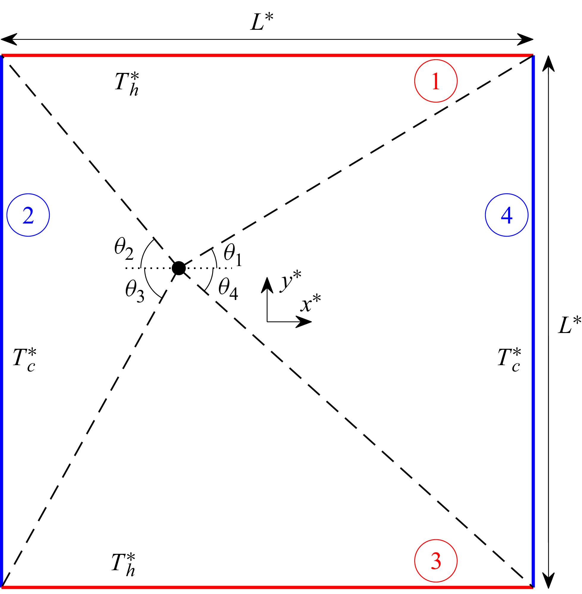
 L∗
 Th∗
 Tc∗
 Th∗>Tc∗
 θi
 i=1,…,4

 Kn=30
 RT=0.2
 RT=0.5

 RT=0.2
 Kn=10
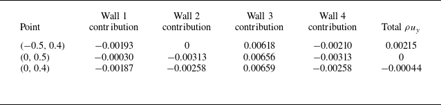
 y^
 ρuy
 RT=0.2
 Kn=5

 y=0.25
 Kn=30,20,10,5
 RT=0.2

 x
 y
 y=0.25
 Kn=20,10
 5
 RT=0.2
 ux
 uy

 RT=0.5
 x
 y
 y=0.25
 Kn=30,20,10
 5
 Kn=20,10and5
 ux
 uy

 Kn
 y=0.25
 RT=0.2
 Kn=10,1,0.1
 0.01

 Kn
 Ek
 RT=0.2
 RT=0.5

 Open access

