3.1. Edge detection

The techniques that will be used in this paper to detect the circles work with edge points. These points of an image are characterised by a quite different value from its neighbours. To highlight these pixels, edge detection techniques are applied (Pajares and de la Cruz, Reference Pajares and de la Cruz2007). First the original coloured image must be transformed into a greyscale one (Kanan and Cottrell, Reference Kanan and Cottrell2012). The result obtained after edge detection is a greyscale image with a black background and edges highlighted in white. After that, this image is transformed into a black and white (binary) image applying Otsu's method (Otsu, Reference Otsu1979). Finally, a morphological operation of dilation to get thicker and crisper lines is applied.

3.2. Circle detection techniques

In this paper, three circle detection techniques have been applied: the well-known Circle Hough Transform (CHT); the method proposed by Silveira (Reference Silveira2005) based on three-edge points, and a new Propagation Method for multiple concentric circles detection based on Circular Regression (PMCR) designed for this purpose.

3.2.1. Circle Hough Transform (CHT)

The Circle Hough Transform (CHT) is a further development of the Hough Transform (Hough, Reference Hough1962), designed for noisy environments.

The Hough transform is a technique originally used on image processing to detect patterns and complex forms in binary images (Illingworth and Kittler, Reference Illingworth and Kittler1988). The basic idea of this method is to transform the data from the image space to a parametric space.

The HT can be applied to any geometric form, including circles. In a two-dimensional space, the circles are described by Equation (1):

(1)$$\lpar x-a\rpar ^2+\lpar y-b\rpar ^2=r^2 $$

where (a, b) is the centre of the circle and r the radius. The parametric space is now defined by three dimensions, (a, b, r), and the crossing point will be in that three-dimensional space. There are multiple variants of the CHT (Yuen et al., Reference Yuen, Princen, Illingworth and Kittler1990) but not all are focused on concentric circles.

3.3. New Propagation Method for multiple concentric circles detection based on Circular Regression

The main problem of the above methods is the computational load and the complexity. Therefore, we propose a new method for multiple concentric circles detection that we have called the Propagation Method, and it is based on circular regression. The process is divided into two steps: detection of the centre and determination of the radius of each circumference.

(1) For centre detection, after the determination of the edges of the image, the points of each edge are used to adjust the circumference that better approximates the cloud of points. This adjustment is performed using a linear square minimum. That is, the problem consists of finding the best circumference that matches a series of points, or finding the values of x ∈ R ² and r ∈ R ⁺ that belong to a set of points a _j ∈ R ², j = 1, 2, …, m, that minimises Equation (2):

(2)$$\min_{x\comma r} \sum_{j=1}^m \lcub F_j\lpar x\comma \; r\rpar \rcub ^{2}$$

where F _j (x, r) is the distance from point a _j to the adjusted circle and x is the centre and r the radius of the circle. The centres beyond the boundaries of the image are discarded, and the others are stored in the array of possible candidates to be used as the input of the algorithm developed to find the real concentric circle centre.

(2) The new concentric circle detection centre works with the coordinates of the candidate centre vector previously obtained. Starting with this data vector, each possible point is evaluated using the general equation of the circumference. The Propagation Method works as follows.

Starting from the candidate centre (a,b), the radar image is scanned for a specific range of radii. For each radius, the corresponding circumference is calculated using Equation (1). The inputs of the function that estimates the radius are the amount of points of the circumference we work with, the interval between the radii that we want to check, and the precision required to identify a circle. The configuration of these input parameters will allow us to detect even incomplete or deformed circles.

Once a circle is drawn on the binarized image, the values of the pixels are evaluated (whether it belongs to an edge or not). Then, if the percentage of white pixels (edges) that match the circles exceeds a previously fixed precision threshold, a circumference of radius r has been found. As the circles must fit entirely in the image, the maximum radius will be half of the shortest side of the image, and the minimum radius is zero. Finally, it is checked that no circle has been counted twice.

The thickness of the circles is not known in advance, therefore the interval between radii is variable. If the distance between two circles that have been detected is smaller than a fixed threshold, only one is considered. The radius of that circle will be the one that has the highest percentage of edge points, because its precision is higher.

3.4. Methods for pattern recognition in radar images

There are different solutions for pattern recognition. For the particular case of radar images, a template matching technique has been selected due to the requirements of designing a fast, reliable and scalable system. The final goal is to develop a strategy that can be used for different radar models in which the scales are previously fixed, and templates can be easily obtained. That is, the possible values to be identified must be limited.

In our case, the FURUNO 1715 radar has the possible values shown in Table 1.

Table 1.

FURUNO 1715 radar scales. Range rings interval (km)

Different algorithms can be applied to calculate the similarity between the original image and the template through the function F. We have selected two, the Sum of Squared Differences (SSD) (Kapadia et al., Reference Kapadia, Chan and Moyé2017) and the Normalised Cross Correlation (NCC) (Briechle and Hanebeck, Reference Briechle and Hanebeck2001), to compare their efficiency for this application.

4.1. Edge detection in radar images

Some of the most common edge detection techniques (Pajares and Cruz, 2007) have been used for image pre-processing. Table 2 summarises the algorithms selected and applied in this study, showing the number of edges detected in each case. Small edges have been discarded because in order to apply the following step of the procedure, at least three points of the circle with enough distance between them are necessary.

Table 2.

Average number of valid edges for circle detection with each operator

A vertical line appeared in most of the images that made it difficult to detect multiple circles due to the continuity of the stroke that generates only a group of lines. Only a Horizontal Sobel filter does not generate that vertical line. According to Table 2, this technique obtains the smallest number of valid edges, thus meaning that it will require fewer edges to analyse, decreasing the processing time.

4.2. Circles detection

The second step is the concentric circles detection. The three methods presented in the previous section have been applied: Circular Hough Transform; three-edge points, and the novel method proposed based on Circular Regression.

The number of detected circles will depend on the edges, and the computational time will depend on the candidate centres found that have to be checked.

4.2.1. Circular Hough Transform

Different algorithms were initially chosen to implement the CHT, but only the solution proposed by Bone (Reference Bone2010) gave good results. This solution has some parameters that need to be adjusted.

In the case here, the whole image has to be analysed, and the range of radii is only limited by the fact that the circles must fit completely within the image, establishing the maximum radius as half of the shortest side of the image. To select the decision threshold, several simulations were run to see how this parameter affects the final results (Figure 1). Although its determination is done by trial and error, once a fixed value is selected, the percentage of circumference that this value represents will depend on its length. That is, the threshold can be defined as a function of the radius. For example, a threshold given by 0·8π r means that 80% of the points of the circumference must belong to an edge.

Figure 1.

Centres obtained with a decision threshold of a) 50%, b) 80%, c) 100%.

As can be observed in Figure 1, when increasing the threshold, the number of detected centres decreases and the precision increases. On the other hand, the computational time is practically the same with any threshold. Taking all of this into account, the selected value was 0·8π r. Using this threshold, the number of detected centres is similar to the one obtained with other more restrictive thresholds, and the accuracy is good.

4.2.2. Detection of concentric circles based on three edge points

The second method used to detect concentric circles is the one based on three edge points. The algorithm goes through each edge searching for three points that meet the condition of minimum distance between them. Thus, the higher the number of points calculated, the larger the computational time.

The thickness of the edges generates a lot of points that are very close to the already found ones, which causes oversampling and slows down the process. To avoid this problem, every time an initial point is evaluated and there are other two that meet a minimum distance condition d _min, the next initial point is chosen at a distance δ _initial. This distance has been determined empirically. The aim is to find enough possible centres to find the real one, but without having too many, which would increase the searching time.

Figure 2 shows the whole process of centre detection.

Figure 2.

(a) Original image, (b) detected centres, (c) valid centres, (d) detected circles using the valid centres.

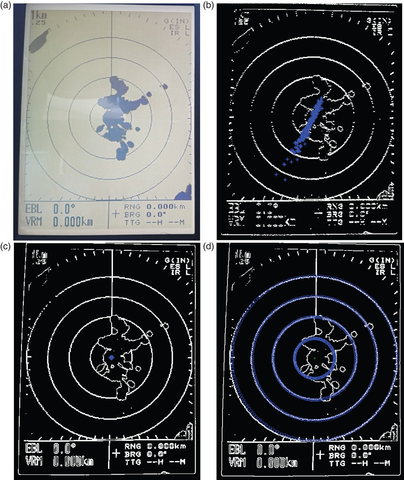
Several simulations with different combinations of δ _initial and d _min were run. The results are shown in Table 3, where the relevant parameters are: centres detected, average number of valid centres, and the average execution time of the circle detection process.

Table 3.

Comparison between different tested configurations

The fastest case (δ _initial = 1, 500) was discarded because only two valid centres were detected, which means that in noisier images it could not detect any centre. Therefore, the chosen configuration for the final tests was δ _initial = 800, δ _initial = 200.

4.2.3. New Propagation Method for multiple concentric circles detection based on Circular Regression

Finally, the third method proposed to detect concentric circles was applied. There are three parameters to be adjusted: (1) accuracy, which indicates the percentage of the detected circle necessary to consider it so; (2) the radius increment, which determines the minimum distance between one radius and the next one in pixels; and (3) the number of points that define each circumference.

These have been analysed independently, starting with the following initial configuration: 35% precision, 0·5 pixel radius increment, and 200 points per circle.

4.2.3.1. Accuracy

Figure 3 shows the results obtained with different precision values. With the initial value, precision  =  35%, all the circles were detected. When this value increases, information is missing, until the precision value reaches 65% where the detection is only occasional. This is due to the fact that the edge extraction method does not obtain perfect circumferences, but sections of them. Therefore, in order not to discard incomplete but valid circles, the value of 35% accuracy was selected.

Figure 3.

Circles detected with a precision of a) 35%, b) 40%, c) 65%.

4.2.3.2. Radius increment

The different values of radius that have been tested are: 0·5, 2 and 5 pixels (Figure 4). It can be observed that, as the radius increases, it is more likely that some circumferences are missing due to the distance between them. Radius increment strongly depends on the thickness of the circles. As in our case the circles are quite thin, it is better to choose the smallest value, that is, 0·5.

Figure 4.

Circles detected with a radius increment of (a) 0·5, (b) 2, (c) 5.

4.2.3.3. Number of points to define a circumference

Figure 5 shows the results for 40, 100 and 200 pixels. The first one is too low, and it fails to detect the smallest circumference of the image because it is partially covered, and the circles are poorly represented. As the number of points increases, all the circumferences are detected and the circles are easier to identify, even when they are partly covered or incomplete, showing a continuous circumference. For the tests, this parameter is set to 200.

Figure 5.

Circles detected for a number of pixels of (a) 40, (b) 100, (c) 200.

4.3. Radar scale recognition results

Template matching was used to identify the radar scale of the real images. Therefore, as patterns are needed, a group of images with good resolution, high contrast and homogeneous luminosity were selected.

Although using individual digits as patterns was an option, results were not good enough. We then used all the possible values of scales as the pattern set, taking advantage of the low number of scales to be recognised (Table 1). The set of patterns is formed by the six different scales values that could be found in the radar image database (Figure 6, top images).

Figure 6.

Maximum value obtained with SSD (red) and NCC (blue) on the same image with all the templates (bottom). At top, the templates.

Two template matching techniques were initially applied in order to compare the results, Normalised Cross-Correlation (NCC) and Sum of Squared Differences (SSD).

Figure 6 shows an example of the results of applying both techniques, NCC and SSD, to each of the available templates of the same radar scale image. The dots, blue for NCC and red for SSD, represent the position of the maximum value obtained by the function F described in Section 3.3. The SSD method was discarded because it was not able to discriminate between patterns and it gave many false positives, obtaining the maximum similarity outside the limits of the radar scale image (this can be seen in Figure 6(a), 6(c) and 6(f), where the red dot does not appear). So, the maximum value of F is obtained by the NCC method (blue dots), and this value is analysed in order to select the best threshold to match the template and the radar scale image.

Several thresholds were tried in applying the NCC method. First it was set to 0·8, high enough to reduce the number of false positives and at the same time significant information is not missed. Using this, 87% of the images were correctly identified, eight were not classified and five were wrongly classified; the average execution time was 1·2 seconds.

The number of hits increases to 95% if the threshold is reduced to 0·65, which is the average value of the maximum NCC for the eight images that generate false negatives. In any case, the small execution time allows this technique to be used in real time applications.

4.4. Circle detection methods comparison and discussion of the results

In this section the results obtained for the whole detection process using the three methods are compared. That is: (1) the Circle Hough Transform; (2) the Three-edge points method; and (3) the new Propagation Method for multiple concentric circles detection based on Circular Regression.

Five representative images from the database out of 100 available images were selected (Figure 7).

Figure 7.

The five images used to evaluate the algorithms.

From left to right and top to bottom, the images contain: (a) four circles with relevant obstructions in the smallest ones; (b) two circles with some occlusion and different degrees of luminosity; (c) two circles and some noise; (d) four circles with a lot of noise; (e) two circles with half of the image covered by a foldable screen, with the aim of showing that the radar could be manipulated by the user and the algorithm still should be able to recognise the circles. This selection covers all the possible situations in terms of luminosity, noise and obstruction.

The criteria to evaluate and compare the proposal are: the execution time in seconds, the number of detected centres, and the number of valid centres of concentric circles. The same computer was used for all of them: an Intel Core i7-3770k 3·5 GHz with 32 Gb RAM, using Windows 7 Professional and the code was developed using the Matlab image processing toolbox.

Tables 4 to 6 show the results obtained with each one of the proposals. For our novel method (Table 6), different configurations were tested changing some input parameters, from the optimum configuration to a suboptimum one. Only the best results are shown in Table 6 to be compared with the other two algorithms.

Table 4.

Results obtained with the Circle Hough Transform

Table 5.

Results obtained with the three-edge points method

Table 6.

Results obtained with the new propagation method based on circular regression

Compared with the three-edge point method (Table 5), the Circle Hough Transform (Table 4) is slower, although it reduces the number of valid centres without losing precision in the detection process. Nevertheless, the time both methods require is too high to be considered for real-time solutions.

The new propagation method for multiple concentric circles detection based on Circular Regression presents a significant reduction of the execution time, and it also reduces the number of valid centres to the minimum without losing precision. Therefore, this proposed solution (Table 6) could be used in real time applications.

5.1. Materials (radar images)

The experimental setup of this application is as follows. A FURUNO 1715 radar (Furuno, 2018) was used, with frequency 9,410 MHz (X-band), horizontal beam width 5·2^°, vertical beam width 25^°, range scales 0·125-24 nm, peak output power of 2·2 kW and with a 7” monochrome Liquid Crystal Display (LCD) display unit.

The final system was implemented in a Raspberry Pi 2 model B (Raspberry Pi, 2018) with a Logitech C920 USB webcam (Logitech, 2018) connected (Figure 8, left).

Figure 8.

Raspberry Pi 2 model B and Logitech C920 USB webcam.

Matlab software was used for the process design but the final system was implemented in the Raspberry Pi using C ++ with the OpenCV library (OpenCV, 2018) for image processing. The camera system was mounted in front of the radar display and both were inside a closed (black) box so that the luminosity of the display was kept constant, avoiding shadows and other spurious effects. This box can be readily and quickly moved out of the way when necessary in order not to limit the human interface with the radar display, allowing the operator to use its own interface through the buttons. Due to necessity of visualise the radar display continuously, both the original image captured by the camera and the processed image, are sent to an external display connected to the Raspberry Pi.

The information is captured by the camera, processed, and a hazard map is generated providing information of the possible obstacles. The final set up is shown in Figure 8, right.

5.2. Image Processing

The processing is based on three modules: (1) Initialisation; (2) Segmentation, and (3) Obstacles detection. Figure 9 shows the procedure.

Figure 9.

Alarm system processing flow.

The initialisation module calculates the centre (C) and radius of the concentric circles (r) according to the new Propagation Method proposed in this paper. The initialisation process runs until an Energy state  =  0 is reached, that is, the difference between consecutive centres is not significant. After that, the scale (S) of the rings is calculated applying the NCC method.

The segmentation module is implemented as explained in Section 3.1.

In the obstacle detection module, the rings and other marks that appear in the edge images are removed according to the data obtained in the initialisation module. Now, only the unidentified objects appear in the image (Figure 10, left). Then, we apply the new propagation technique, using the found centre (red dot) and propagating the circles up to the maximum radius (Figure 10, right).

Figure 10.

Final image with the unidentified objects and without circles and marks (left); radius propagation with the new technique (right).

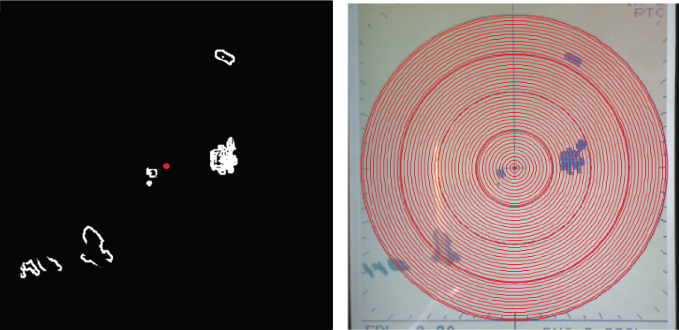
When a circle's point detects an edge, we calculate the Euclidean distance in pixels and the angle in radians between this point (Px, Py) and the centre of the circles (Cx, Cy). Now, knowing the metric radar scale that has been calculated in the initialisation module and the radius of the outer concentric circle, we can convert the distance from pixels to the metric scale.

Our algorithm has been designed to identify the nearest object both in the whole image and also within a selected cone, so the human operator can select a particular area to get alarms when the closest object appears in that zone (Figure 11).

Figure 11.

Object detection with different scales. The red dot identifies the nearest object in the cone, and the white dot the nearest object in the whole image. (a) outer radius 1 km (b) outer radius 250 metres.

If the objects are closer than a pre-defined distance, the alarm system is activated, and it can send a message to a mobile phone or tablet connected via Wi-Fi, or by broadcasting a sound.

5.3. Distance measurement validation

To evaluate the precision with static objects, we used a cylindrical buoy which was positioned by the Global Positioning System (GPS). Later, a kayak equipped with our vision system and a GPS was used to navigate around this buoy and to take pictures. The GPS coordinates and the images were stored in a Secure Digital (SD) card to measure the distance and to compare the GPS and radar measurements (Figure 12, left). The error in 100 of the captured images can vary up to 5·76 m with an average difference of 1·93 m (Figure 12, right).

Figure 12.

GPS-radar distance comparison.

This difference is considered valid for navigation purposes. Objects were detected at long distances, further than 10 m. For lower distances, this radar system would not be appropriate.

This technique can be used for different scales. As is shown in Figure 11, the same object is identified within the cone with two different scales. Its distance and angle are similar, in fact they only vary 1 m and 4^° respectively from one to another.

5.4. Processing time

The processing time varies with the distance of the object. The farther the object is, the longer it takes, because it is a circle propagation technique. In Table 7, objects belonging to four representative classes with different scale rings are shown. Objects in groups 2 and 4 are closer to the outer circle, and objects belonging to group 1 and 3 appear near the middle circles. The scale is selected manually by the operator and the initialisation module configures the radar to detect objects at different distances.

Table 7.

Computational detection time at difference distances

Computation time represents the average time that the object detection requires at that particular distance for 100 of the captured images. All objects belonging to a group are placed at approximately the same distance (detection distance), which differs with the object distances of another group.

The antenna speed for a short pulse has a rotation speed of 41 rpm, so for one complete scanning (360^°) it takes 1·5 seconds. In the worst case, the processing time allows up to six frames per second (fps), so this system can detect an object in real-time and it is not necessary to wait for a complete scan.