Wing–antenna interaction reduces odour fatigue in butterfly odour-tracking flight

Zhipeng Lou; Menglong Lei; Haibo Dong; Chengyu Li

doi:10.1017/jfm.2024.644

Wing–antenna interaction reduces odour fatigue in butterfly odour-tracking flight

Published online by Cambridge University Press: 04 November 2024

and

Zhipeng Lou: Affiliation:
Department of Mechanical & Aerospace Engineering, Case Western Reserve University, OH 44106, USA
Menglong Lei: Affiliation:
Department of Mechanical & Aerospace Engineering, Case Western Reserve University, OH 44106, USA
Haibo Dong: Affiliation:
Department of Mechanical & Aerospace Engineering, University of Virginia, Charlottesville, VA 22903, USA
Chengyu Li*: Affiliation:
Department of Mechanical & Aerospace Engineering, Case Western Reserve University, OH 44106, USA
*: †Email address for correspondence: cxl1692@case.edu

Article contents

Abstract
Introduction
Methodology
Results and discussion
Conclusions
Declaration of interests
Data availability
References

Rights & Permissions

Abstract

Flying insects exhibit remarkable capabilities in coordinating their olfactory sensory system and flapping wings during odour plume-tracking flights. While observations have indicated that their flapping wing motion can ‘sniff’ up the incoming plumes for better odour sampling range, how flapping motion impacts the odour concentration field around the antennae is unknown. Here, we reconstruct the body and wing kinematics of a forwards-flying butterfly based on high-speed images. Using an in-house computational fluid dynamics solver, we simulate the unsteady flow field and odourant transport process by solving the Navier–Stokes and odourant advection-diffusion equations. Our results show that, during flapping flight, the interaction between wing leading-edge vortices and antenna vortices strengthens the circulation of antenna vortices by over two-fold compared with cases without flapping motion, leading to a significant increase in odour intensity fluctuation along the antennae. Specifically, the interaction between the wings and antennae amplifies odour intensity fluctuations on the antennae by up to 8.4 fold. This enhancement is critical in preventing odour fatigue during odour-tracking flights. Further analysis reveals that this interaction is influenced by the inter-antennal angle. Adjusting this angle allows insects to balance between resistance to odour fatigue and the breadth of odour sampling. Narrower inter-antennal angles enhance fatigue resistance, while wider angles extend the sampling range but reduce resistance. Additionally, our findings suggest that while the flexibility of the wings and the thorax's pitching motion in butterflies do influence odour fluctuation, their impact is relatively secondary to that of the wing–antenna interaction.

JFM classification

Biological Fluid Dynamics: Swimming/flying

Information

Type: JFM Papers
Information: Journal of Fluid Mechanics , Volume 998 , 10 November 2024, A45
DOI: https://doi.org/10.1017/jfm.2024.644 [Opens in a new window]
Creative Commons: This is an Open Access article, distributed under the terms of the Creative Commons Attribution licence (http://creativecommons.org/licenses/by/4.0), which permits unrestricted re-use, distribution and reproduction, provided the original article is properly cited.
Copyright: © The Author(s), 2024. Published by Cambridge University Press

1. Introduction

Flying insects, as products of natural engineering, are tiny yet equipped with advanced features: highly efficient flapping wings (Heinrich Reference Heinrich1974; Lehmann, Dickinson & Patel Reference Lehmann, Dickinson and Patel1997; Jones & Babinsky Reference Jones and Babinsky2012; Lehmann, Wang & Engels Reference Lehmann, Wang and Engels2021), robust flight control (Fry, Sayaman & Dickinson Reference Fry, Sayaman and Dickinson2003; Iwamoto & Yagi Reference Iwamoto and Yagi2013; Dickinson & Muijres Reference Dickinson and Muijres2016; Farisenkov et al. Reference Farisenkov, Kolomenskiy, Petrov, Engels, Lapina, Lehmann, Onishi, Liu and Polilov2022) and sophisticated sensory neural networks (Taylor & Krapp Reference Taylor and Krapp2007; Rapp & Nawrot Reference Rapp and Nawrot2020; Tuckman et al. Reference Tuckman, Kim, Rangan, Lei and Patel2021). The collaboration of these features allows insects to precisely navigate in a complex flow environment. To gain inspiration on artificial insect-like systems, scientists endeavour to understand these complex mechanisms of collaborations (Ashley & Rodden Reference Ashley and Rodden1972; Lehmann, Sane & Dickinson Reference Lehmann, Sane and Dickinson2005; Ruiz & Theobald Reference Ruiz and Theobald2020; Hürkey et al. Reference Hürkey, Niemeyer, Schleimer, Ryglewski, Schreiber and Duch2023). While insects are managed to coordinate these functions for complex tasks, current man-made designs are facing challenges in integrating these features. For example, even equipped with highly sensitive sensors, rotary drones have trouble detecting chemicals because of the strong induced flow in downwash, which blows away most of the chemicals (Allers et al. Reference Allers, Ahrens, Hitzemann, Bock, Wolf, Radunz, Meyer, Wilsenack, Zimmermann and Ficks2023). This limitation makes odour-detection drones ineffective and even dangerous to work at places where hazardous chemicals have risks of spreading out. In contrast, insects have a fundamental ability of not blowing away these chemicals, especially when odour detection is the main purpose of the flight, such as during foraging or mating. Compared with current drone designs, insects stroke their flapping wings to keep aloft instead of rotary blades. Understanding the mechanism of how insects coordinate their wing flapping motion and olfactory perception is necessary for replicating the chemical detection performance in designs of unmanned devices navigating in dynamic flow environments.

1.1. Olfactory sensory and flying are not conflicting for insects

Olfactory sensory while flying is an essential ability of insects which is crucial for foraging, mating, and communication (Baker Reference Baker1989; Baker et al. Reference Baker, Dickinson, Findley, Gire, Louis, Suver, Verhagen, Nagel and Smear2018; Lin Reference Lin2023). However, during an odour plume-tracking flight, the flapping motion of insects’ wings inevitably disturbs the surrounding air due to the generation of wing-induced flow. The disturbance of the flow field can potentially blow away the incoming odour plume, causing the failure of odour sensory, just like the failure of rotary drones for odour detection. Recent research has shown that when insects fly under a high reduced frequency, the induced flow redirects the plume to flow above the antennae by forming a shield-like streamline in the frontal flow field (Lei & Li Reference Lei and Li2023). It is true that such induced flow reduces the plume reachable by antennae, which has a negative effect on odour perception. However, this shielding effect serves other benefits – increasing the odour sampling range. This is desirable when insects are flying in the mode called cross-wind zigzagging – a flight mode when the insects need larger sampling due to lost odour clues. This active motion can be analogous to ‘sniffing’ in mammals (Tripathy et al. Reference Tripathy, Peters, Staudacher, Kalwar, Hatfield and Daly2010). Conversely, during an upwind surging flight – the other mode that requires stable track of odour clue – insects prioritize strengthening peak odour intensity over antennae, sacrificing the odour sampling range. Evaluating the odour intensity over the antennae of fruit flies during forwards flights, Li, Dong & Zhao (Reference Li, Dong and Zhao2018) reported that the wing-induced flow enhances the peak odour flux over the antennae up to 1.8 times. By switching wing kinematics between two flight modes, insects can strategically track the odour source. This adaptability enables insects to locate odour sources in complex environments with obstacles, weak odour fields and natural disturbance (Wolf Reference Wolf2011; Conchou et al. Reference Conchou, Lucas, Meslin, Proffit, Staudt and Renou2019; Lei & Li Reference Lei and Li2023).

1.2. Olfactory adaptation

In addition to the ability to ‘sniffing’ odourants without dispersing them, insects still have a weakness that is shared with mammals: continuous odour stimulus will lead to olfactory adaptation, commonly known as odour fatigue. Unlike artificial odour sensors (Wen et al. Reference Wen, Luo, He and Mei2018), insects’ sensilla neurons can reach an adapted state under continuous stimuli (Dolzer, Fischer & Stengl Reference Dolzer, Fischer and Stengl2003). Experimental observations have revealed that moths show a better response to pulsatile odour delivery compared with constant odour stimuli (Baker et al. Reference Baker, Willis, Haynes, Phelan, Haynes, Phelan, Haynes and Phelan1985; Dolzer et al. Reference Dolzer, Fischer and Stengl2003; Daly et al. Reference Daly, Kalwar, Hatfield, Staudacher and Bradley2013). However, under steady odour delivery, moths have poor sensory performance. Sanders (Reference Sanders1997) conducted an experiment where a moth is navigating in a high-concentration field of pheromone, and it loses track of the pheromone source. The main reason for the failure is that the stimuli intensity is so much stronger than in a natural environment that the moth senses a relatively constant odour intensity that causes odour fatigue.

In nature, to locate odour sources in complex environments, insects must have mastered some mechanisms that help them overcome odour fatigue. For example, as insects swarm – a mating and pairing activity for many insects (Syrjämäki Reference Syrjämäki1964; Sullivan Reference Sullivan1981) – insects must have a way to track the pheromone plume under continuous pheromone stimuli without getting odour fatigue. We hypothesize that insects’ ability to navigate in such concentrated pheromone fields may be the result of the beneficial flapping motion. Several experiments have shown some hints that induced airflow, a byproduct of flapping flight, varies linearly with wing beat frequency and alters the olfactory stimuli received by the sensory organs (Sane Reference Sane2006; Sane & Jacobson Reference Sane and Jacobson2006). This induced airflow potentially creates fluctuations, preventing the sensory neurons from reaching an adapted state. However, to date, there is a lack of comprehensive explanation that attributes the mechanism of the odour fatigue resistance to the flapping motion, especially from a fluid mechanic perspective.

1.3. Wing-induced flow on olfactory perception

During flight, the existence of antennae and wing-induced flow have a mutual influence: the structure of antennae may disturb the induced flow, while flow affects sensory perception. For example, much research found that the rami density of pectinate antennae (comb-like structure) among insects, like moths, effectively affects how much the air can flow through the sensilla, influencing the pheromone capture (Jaffar-Bandjee et al. Reference Jaffar-Bandjee, Steinmann, Krijnen and Casas2020a,Reference Jaffar-Bandjee, Steinmann, Krijnen and Casasb). In contrast, the wing-induced airflow can decrease the depth of the velocity boundary layer over antennae and thereby increase the rate of interception of air-born olfactory cues by at least an order of magnitude (Loudon & Koehl Reference Loudon and Koehl2000; Loudon & Davis Reference Loudon and Davis2005). Although current researchers have noticed the antennae themselves may affect the flow, most research still only treats the antennae of insects as proprioceptors, providing speed feedback to insects (Roy Khurana & Sane Reference Roy Khurana and Sane2016). The inter-antennal angle, the angle between two antennae, is used to estimate the airspeed in experiments (Schneider Reference Schneider1964).

Recent research has observed that when insects land on odour sources, they actively vibrate their antennae to enhance sensory sampling (Schneider Reference Schneider1964; Loudon Reference Loudon2009; Dürr, Berendes & Strube-Bloss Reference Dürr, Berendes and Strube-Bloss2022). We speculate that this antennal movement can induce fluctuations in the air, affecting the distribution of odour plumes. Such fluctuations are crucial for preventing odour fatigue, particularly as insects land on odour sources. However, insects exhibit different behaviour during flight, where antennae remain relatively fixed at certain angles to maintain flight stability (Krishnan et al. Reference Krishnan, Prabhakar, Sudarsan and Sane2012). Frequent movement of antennae may break the balance of inertial forces, making the flight unstable. Thus, aside from the benefits of antennal movements, odour fatigue resistance may also be attributed to the induced flow from wing flapping motion, termed wing–antenna interaction. Considering that the induced flow has been found to provide some benefits for odour perception, flapping motion can serve as an alternative to antennal movement during flight.

1.4. Other impact factors: body motion and wing flexibility

Many factors can influence the odour perception of antennae, potentially mitigating odour fatigue. One such factor is body motion. Based on observations, some insects exhibit periodic body rotations during odour-tracking flights. The oscillation of the butterfly's body has been found to actively influence the direction of vortex rings generated by flapping wings (Fei & Yang Reference Fei and Yang2016) and enhance aerodynamic performance (Chang et al. Reference Chang, Lai, Lin and Yang2020). As antennae are fixed on the head during the flight for balance purposes, body motion leads to relative antennal motion against the global coordinates. When the antennae intersect the air flow, corresponding air disturbances may generate fluctuations in the odour field, potentially preventing odour fatigue. However, the specific impact of body motion on odour perception remains unexplored.

Another factor is wing flexibility. In contrast to rigid wings, the deformation of flexible wings facilitates the transfer of wing momentum to the wake, directing a more effective direction of aerodynamic forces according to the flight direction (Young et al. Reference Young, Walker, Bomphrey, Taylor and Thomas2009). This ability to direct airflow backwards during forwards flight potentially mitigates backflow that disperses incoming plumes. However, further investigation is required to confirm this speculation as the impacts of other aforementioned factors are explored.

1.5. Modelling the free-flying butterfly and numerical simulations

Butterflies offer a unique opportunity to study both flight aerodynamics and olfactory sensing. Their signature long antennae allow easier analysis of flow dynamics and potential interactions with wings due to the relatively low ratio between antenna length and wingspan. Compared with other species such as moths and locusts, butterflies typically have low-aspect-ratio wings, with aspect ratios (ARs) ranging from 1.5 to 2.5 (Betts & Wootton Reference Betts and Wootton1988; Dudley & Srygley Reference Dudley and Srygley1994; Tanaka & Shimoyama Reference Tanaka and Shimoyama2010). Compared with high-aspect-ratio wings (AR > 3) of other insects, flapping wings under low AR results in stronger wingtip vortices and increased air perturbation, facilitating clearer observations of wing-induced flow (Le Roy, Debat & Llaurens Reference Le Roy, Debat and Llaurens2019). Additionally, butterflies commonly use a combination of thorax-pithing and abdominal oscillation with wing flapping, setting them apart from other insects. Furthermore, the aerodynamic effects of wing deformation in butterflies are well-studied due to their relatively higher wing flexibility, allowing for a more focused investigation of its impact on olfactory performance.

To address our speculations, we first reconstructed the kinematics of flapping wings and oscillating bodies based on high-speed videos of forwards-flying butterflies. We specifically selected an upwind surging butterfly for analysis to simplify the investigation by excluding complex flight manoeuvres during zigzagging flights. Employing an in-house high-fidelity computational fluid dynamics (CFD) solver, we explored the unsteady flow field and odourant transport process by solving both the Navier–Stokes and advection-diffusion equations.

A series of comprehensive parametric studies were conducted to investigate how or whether wing-induced flow resulting from wing-antenna interaction can prevent odour fatigue. Our aim was to address these questions from a fluid mechanics perspective: (i) how or whether wing-antenna interaction can prevent odour fatigue, (ii) how or whether inter-antennal angles can modulate the wing-antenna interaction mechanism, and (iii) what extent flexible wing pairs and varying thorax pithing contribute to odour fatigue resistance.

2. Methodology

2.1. Reconstruction of freely flying butterfly

Monarch butterflies (Danaus plexippus) were wild captured and expected to fly into a filming scene voluntarily. The filming scene consisted of three orthogonally calibrated high-speed video apparatus (Photron Fastcam SA3 60 K, Photron USA, Inc, San Diego, CA, USA) with a shutter speed of 1/(20 000) s and a resolution of 1024 × 1024 pixels. Three orthogonal whiteboards were set as backgrounds placed towards each camera. We collected approximately 20 separate recordings of free-flying butterflies at 1000 frames per second. One recording was selected when the butterfly was performing a forwards flying at a constant speed (0.85 m s⁻¹). The morphological parameters of the corresponding butterfly are summarized in table 1.

Table 1.

Morphological parameters of the monarch butterfly (Danaus plexippus). *The parameters in the table are listed for one side of the wings.

To reconstruct the freely flying butterfly, we adopted a template-based hierarchical subdivision surface method with joint controllers using Autodesk MAYA (Autodesk, San Raphael, CA, USA). Figure 1 compares the real butterfly with our model with a template mesh. Morphologically, a butterfly has a forewing and a hindwing on each side. During flight, the forewing and hindwing partially overlap with each other serving as a single lifting surface. To reduce computational complexity in CFD simulation, the forewing and the hindwing were modelled as one piece in the current study. A similar modelling approach has also been adopted in previous studies (Yokoyama et al. Reference Yokoyama, Senda, Iima and Hirai2013; Zheng, Hedrick & Mittal Reference Zheng, Hedrick and Mittal2013; Bode-Oke & Dong Reference Bode-Oke and Dong2020). Figure 2(a) demonstrates the reconstruction process at a selected instant. The high-speed videos were loaded into the virtual cameras based on the experimental set-up. The wing and body kinematics were applied to the model according to the two-dimensional (2-D) images (figure 2b,c).

Figure 1.

(a) Monarch butterfly (Danaus plexippus) with the computational model on the left half. (b) Schematic of the joint controllers for adjusting surface deformation.

Figure 2.

(a) Scaled virtual scene based on the actual filming scene. Reconstructed model overlapping with the background images from (b) side view and (c) back view, at a selected instant. See the supplementary movie 1 for the entire reconstructed flapping flight motion.

The surface of the model was controlled by a set of joint controllers of the template model. Each of the joints governs the nearby meshes. The relationship of the joints is established on a hierarchy of ‘parent’ and ‘child’, where parent joints control the child joint controllers. By rotating one joint against the centre of itself, for example, the assigned nearby meshes rotated against the centre, and all its child joints rotated against this parent joint. The joint controllers on wings are set based on the easily identifiable natural patterns of wing veins. On the body, we put a parent joint controller on the centre of mass of the butterfly and a child controller on the abdomen hinge to control the whole abdominal oscillation. Before any kinematics and deformation were applied, the initial pose of all wing joints was set as shown in figure 1(b), and the initial mesh was planar as the template wing mesh (figure 1a). By manipulating the joint controllers, we reconstructed the three-dimensional (3-D) wing and body kinematics with natural deformations at 91 instants during one flapping cycle. The morphology of the model butterfly's wings was adjusted to align with the high-speed recordings (see figure 2(b,c) and supplementary movie 1 is available at https://doi.org/10.1017/jfm.2024.644). Between the 91 reconstructed frames, we use Fourier interpolation to interpolate the unstructured surface mesh over time, producing a high temporal frequency (960 time steps per beating cycle) input for our CFD solver.

2.2. Quantification of wing and body kinematics

The wing kinematics are described by three Euler angles in a reference frame fixed on the stroke plane (figure 3a). The stroke plane is obtained by the least-squares plane of the wing root and the wing tip trajectory. Next, wing kinematics were quantified on the stroke plane using three Euler angles: wing stroke, wing deviation and wing pitch. The wing stroke angle (ψ_w) provides the location of the wing in the stroke plane, defined as the angle between the projection of the root-to-tip connection line and the z_w axis. The deviation angle (ϕ_w) is the angle between the root-to-tip connection line and its projection onto the stroke plane. The wing pitch angle (θ_w) provides the angle between the wing chord and the stroke plane.

Figure 3.

(a) Definition of wing Euler angles (wing pitch angle θ_w, wing deviation angle ϕ_w, wing stroke angle ψ_w) in a local coordinate system (x_w, y_w, z_w). The origin (O_w) is located at the wing root. The wing position shown here is at the mid-downstroke. Additionally, θ_w is smaller than 90° when leading-edge points forwards; ψ_w = 0° when the wing tip points along z_w and ψ_w < 0° when the wing tip is at the dorsal side of the body. The value of ϕ_w is positive when the wing tip is above the stroke plane. (b) Time course of Euler angles for the forewing. (c) Time course of Euler angles for the hindwing. Due to the spanwise twisting, the variation of wing pitch angle (θ_w) in (b) and (c) are shown with standard deviations.

As shown in figure 3(b,c), the Euler angles of the butterfly's forewing and hindwing are plotted separately due to the dramatic surface deformation in flapping flight. In one flapping cycle, the forewing stroke angle (ψ_w) has an amplitude of 146.53° (−88.12° to 58.41°), while the hindwing has an amplitude of 117.76° (−40.98° to 76.78°). The forewing and hindwing approach the peak stroke angles at a similar time, indicating similar stroke phases.

The forewing deviation angle (ϕ_w) is positive most of the time, which ranges from −4.88° to 27.01°. However, the hindwing deviation angle has both positive and negative values, which range from −12.40° to 17.93°. The changing magnitude of the forewing and hindwing deviation angles are 31.89° and 30.33°, which are relatively close.

The wing pitch angles (θ_w) are calculated based on the wing chords at 25 %, 50 %, and 75 % of the wingspan, and the plotted curves are the average value with standard deviations. Within the flapping cycle, the forewing pitches range from 63.49° to 134.89° while the hindwing pitch angle ranges from 33.57° to 170.96°. The pitch amplitude of the forewing and hindwing are 71.4° and 137.39°, respectively. The forewing reaches a valley of pitch angle 25 % period sooner than the hindwing, indicating the pitching of the hindwing lags the forewing.

The general patterns of wing Euler angles, including the flapping amplitude and stroke period reported in our study align with findings from several other butterfly studies (Senda et al. Reference Senda, Obara, Kitamura, Yokoyama, Hirai and Iima2012; Yokoyama et al. Reference Yokoyama, Senda, Iima and Hirai2013; Zheng et al. Reference Zheng, Hedrick and Mittal2013). For example, our reported wing position angle agrees with observations from the monarch butterfly study conducted by Sridhar, Kang & Landrum (Reference Sridhar, Kang and Landrum2016). When averaging the stroke angle for both the forewing and hindwing, we obtain a range of −64.55 to 67.60°, resulting in an amplitude of 132.15°. This amplitude range is consistent with Sridhar's reported values falling within the range of 76° to 151°, derived from multiple flapping cycles and the average values of forewing and hindwing. A key variation among these studies is in the peak or valley pitch angle. While some studies pinpoint the middle of the downstroke, others indicate the beginning of the downstroke. In our investigation, the valley pitch angle, obtained by averaging the forewing and hindwing, closely aligns with the mid-point of the downstroke. The observed variation in pitch angle phase is reasonable, especially considering that the measurement of pitch angle depends on the location along the wingspan. Our study goes a step further by reporting pitch angles based on three distinct locations, contributing to a more comprehensive understanding of the phase dynamics.

The reconstruction of the freely flying butterfly with both surface deformation and wing–body coupled oscillation is defined as the baseline model throughout the paper. To evaluate the influence of wing flexibility, we also constructed a rigid wing model for comparison with the baseline model. The mesh and controller set of the rigid wing model are planar as the template mesh shown in figure 1(a). We kept the kinematics of the root joints (figure 1b) identical between both models, and we attempted to match the forewing leading-edge of the rigid model to that of the baseline model. Thus, the wing root, the node on the leading edge and the trailing edge at 1/2 wingspan of both models overlap. The hindwing was flattened onto the plane of the rigid forewing and attached to it through the whole flapping cycle. Figure 4 shows the wing kinematics of the rigid wing model.

Figure 4.

Time course of Euler angles for the forewing and hindwing of the rigid wing model.

The butterfly uses a coupled wing–body motion to fly. To describe the body kinematics, two Cartesian coordinate systems were introduced: a global frame (x, y, z) and a body frame (x_b, y_b, z_b). The body frame was fixed to the mid-frontal plane with an origin located at the centre of mass of the butterfly (figure 5a). During a forwards flight, the body rolling and yawing are negligible. Thus, the body motion can be described only by the thorax pitch angle θ_t and the centre of rotation positioned at the thorax centre (midpoint of two wing roots). To quantify the abdominal oscillation, the abdomen deviation angle θ_a is defined in figure 5(b). It represents the relative position of the abdomen with respect to the mid-frontal plane. The θ_a is positive when the abdomen is bent below the mid-frontal plane. As shown in figure 5(c), the body thorax pitches downwards during the downstroke of flapping wings, while it pitches upwards during the upstroke. In the meanwhile, the abdomen first pitched down during the first half downstroke and then pitched up. The position of the abdomen gradually recovers to the initial position during the upstroke of flapping wings. It is worth noting that there is a phase difference of 20 % period between the thorax pitch angle (θ_t) and abdomen deviation angle (θ_a), as shown in figure 5(c). The body kinematics data reported here are consistent with a previous butterfly study (Fei & Yang Reference Fei and Yang2016). To demonstrate the wing kinematics in the global frame, figure 6(a) presents the wingtip trajectory with body oscillation in flapping flight. The associated wing chord position with respect to the horizontal plane is shown in figure 6(b).

Figure 5.

(a) Definition of the mid-frontal plane which crosses the wing–body intersection. The longitudinal axis is in the mid-frontal plane and goes through both head and thorax–abdomen intersection. The direction y_b+ follows the dorsoventral direction. (b) Definition of thorax pitch angle (θ_t) and abdomen deviation angle (θ_a). The thorax pitch angle is the angle of the body's longitudinal axis against the horizontal plane in the global frame. The abdomen deviation angle is defined as the angle between the abdominal axis and the thorax longitudinal axis. The θ_a is positive when the abdomen is bent below the mid-frontal plane. (c) Time history of thorax pitch angle (θ_t) and abdomen deviation angle (θ_a). The grey-shaded region indicates the downstroke period of flapping wings.

Figure 6.

(a) Body oscillation and wing tip trajectory in a global coordinate system. (b) Schematics for wing chords. The blue wing cord lines represent the downstroke and the red ones represent the upstroke, where the filled circles on each cord line stand for the leading-edge.

2.3. Numerical method

This study employs an immersed-boundary-method-based in-house CFD solver to numerically solve the 3-D unsteady Navier–Stokes equations for a viscous incompressible flow with constant properties given by

(2.1)

\begin{gather}\frac{{\partial {u_i}}}{{\partial {x_i}}} = 0,\end{gather}

(2.2)

\begin{gather}\frac{{\partial {u_i}}}{{\partial t}} + \frac{{\partial ({u_i}{u_j})}}{{\partial {x_j}}} =- \frac{1}{\rho }\frac{{\partial p}}{{\partial {x_i}}} + \nu\frac{\partial }{{\partial {x_j}}}\left( {\frac{{\partial {u_i}}}{{\partial {x_j}}}} \right),\end{gather}

where u_i (i = 1,2,3) are the velocity components in the x-, y- and z-directions, respectively; p is the pressure; $\rho $ and $\nu$ are the fluid density and kinematic viscosity, respectively.

The above equations are discretized using a cell-centred collocated grid arrangement of the primitive variables (u_i and p). The fractional step method is used to integrate the equations in time, and a second-order central difference scheme is used in space. An immersed-boundary-method-based approach is applied to handle the complex moving boundaries of the beating wings. In this method, boundary conditions are imposed on the immersed boundaries through a ghost-cell procedure. Compared with the boundary-conforming methods, the immersed-boundary-method approach eliminates the need for complicated re-meshing algorithms. It thus significantly reduces the computational cost associated with simulating flow past complex moving boundaries. Immersed boundary methods can be broadly characterized under two categories: continuous forcing approach (Goldstein, Handler & Sirovich Reference Goldstein, Handler and Sirovich1993) and discrete forcing approach (Kim, Kim & Choi Reference Kim, Kim and Choi2001). The present study employs a multi-dimensional ‘ghost-cell’ methodology to impose the boundary conditions on the immersed boundary (Mittal et al. Reference Mittal, Dong, Bozkurttas, Najjar, Vargas and von Loebbecke2008). This method can be categorized as a discrete forcing approach wherein forcing is directly incorporated into the discretized Navier–Stokes equations. The movement of the immersed boundaries (wings and body) is prescribed according to the image-based reconstruction as described in § 2.1. This immersed-boundary method has successfully been used to simulate insect flights (Li et al. Reference Li, Dong and Zhao2018; Li, Dong, & Cheng Reference Li, Dong and Cheng2020a; Li Reference Li2021) and bio-inspired propulsions (Li & Dong Reference Li and Dong2016; Li et al. Reference Li, Wang, Liu, Deng and Dong2019; Li, Dong, & Zhao Reference Li, Dong and Zhao2020b; Lei, Crimaldi & Li Reference Lei, Crimaldi and Li2021). Validations of the current in-house CFD solver can be found in our previous studies (Li, Dong & Liu Reference Li, Dong and Liu2015; Li & Dong Reference Li and Dong2017; Li et al. Reference Li, Jiang, Dong and Zhao2017; Lei & Li Reference Lei and Li2020; Lionetti, Hedrick & Li Reference Lionetti, Hedrick and Li2022).

The governing equation of odourant advection-diffusion in the air phase can be written as

(2.3)

\begin{equation}\frac{{\partial C^{\prime}}}{{\partial t}} + {U_i}\frac{{\partial C^{\prime}}}{{\partial {x_i}}} = D\frac{{{\partial ^2}C^{\prime}}}{{\partial {x_i}\partial {x_i}}},\end{equation}

where i (= 1, 2 and 3) indicates the components in the x-, y- and z-directions;$C^{\prime} = C/{C_0}$ is the normalized odour intensity and ${C_0}$ is the odour intensity of the odour source; ${U_i}$ is the face-centred velocity obtained by interpolation of the cell-centred velocity ${u_i}$; D is the odour diffusivity.

At each time step, the odour advection-diffusion equation is solved based on the velocity field obtained from the Navier–Stokes equations to obtain the odour concentration landscape. The advection-diffusion equation is discretized using an implicit method with second-order accuracy in space. The detailed validations of this numerical treatment for solving odour transportation have been documented in our previous study (Lei et al. Reference Lei, Crimaldi and Li2021).

2.4. Simulation set-up

Figure 7(a) illustrates the simulation set-up for the current study. The inflow boundary condition was specified at the front of the fluid domain, and an outflow boundary condition was used at the back of the fluid domain. At all other lateral boundaries, a zero gradient was adopted. The domain mesh has two refined layers. A very fine mesh is provided in a cubic region around the butterfly's body and wings. Around this region, there is a secondary denser mesh. Beyond these refined layers, the mesh grid is stretched rapidly. The simulations were carried out with a grid size of 289 × 177 × 225. The simulation results are independent of grid size, which is validated by the comparison of results with different grid resolutions. Figure 7(b) plots the comparison of the lift and drag forces among the baseline grid and two additional grid set-ups, where a finer grid with the size of 353 × 193 × 257 and a coarse grid with the size of 257 × 153 × 277 are tested for the comparison. There are less than 3 % differences between the testing cases and the baseline case, which indicates that the results are independent of grid size.

Figure 7.

(a) Schematic of the computational mesh and boundary conditions employed in the current simulation. (b,c) Comparison of lift coefficient $({C_L})$ and drag coefficient $({C_D})$ for demonstrating the grid independence of the computed results. The grid employed in simulations is 257 × 153 × 277 = 1.08 × 10⁷ (coarse), 289 × 177 × 225 = 1.30 × 10⁷ (intermediate) and 353 × 193 × 257 = 1.75 × 10⁷ (finer).

The flow field is characterized by Reynolds number $(Re)$. In the current study, the Reynolds number is defined by $Re = {U_\infty }R/\nu$, where ${U_\infty }$ is the forwards flight velocity, R is the wingspan length and $\nu$ is the kinematic viscosity (approximately $1.56 \times {10^{ - 5}}\;{\textrm{m}^2}\;{\textrm{s}^{ - 1}}$ for air at a room temperature of 25 °C). Based on the experimental measurement (table 1), the Reynolds number is 2446.47.

The odourant transport phenomenon is characterized by both Re and Schmidt number $(Sc)$, which are combined as the Péclet number $(Pe = Re\,Sc)$. Here, the Péclet number is 1736.99, which indicates a ratio between the rate of advection and the rate of diffusion. With the Péclet number of the order of 10³, the advective odour transportation is faster than the diffusive odour transportation. The Schmidt number is a ratio between kinematic viscosity and odour diffusivity $(Sc = \nu/D)$. The typical natural odour has relatively low diffusivity (D) in the air at normal temperature and pressure, and is of an order of ${10^{ - 5}}\;{\textrm{m}^2}\;{\textrm{s}^{-1}}$. In this study, the odour diffusivity D is set to $2.2 \times {10^{ - 5}}\;{\textrm{m}^2}\;{\textrm{s}^{ - 1}}$ which leads to a Schmidt number Sc of 0.71.

During the simulations, a cubic odour source is positioned in front of the butterfly model at a distance of 1.27R (wingspan). The odour source's centre aligns with the coordinates of the thorax centre when the thorax pitch angle (θ_t) is 44.07°, a value derived from the average of the peak and valley of θ_t.

2.5. Evaluation of aerodynamic performance and olfaction sensitivity

The aerodynamic forces are obtained by the surface integration of pressure and shear stress across the wings and the body. In this study, the vertical and horizontal components of aerodynamic force $({\boldsymbol{F}_{aero}})$ are denoted by the scalars: lift $({F_L})$ and drag $({F_D})$, which are calculated by projecting the integrated force in the vertical and horizontal directions, respectively. The lift and drag force are expressed as non-dimensional scalar coefficients, lift coefficient $({C_L})$ and drag coefficient $({C_D})$, as defined by the following equations:

(2.4)

\begin{gather}{C_L} = \frac{{{F_L}}}{{{\textstyle{1 \over 2}}\rho U_\infty ^2{S_w}}},\end{gather}

(2.5)

\begin{gather}{C_D} = \frac{{{F_D}}}{{{\textstyle{1 \over 2}}\rho U_\infty ^2{S_w}}}.\end{gather}

Here $\rho = 1.2\ \textrm{kg}\ {\textrm{m}^{ - 3}}$ represents the air density, ${U_\infty }$ is the flight velocity, and ${S_w}$ is the total area of the forewing and hindwing.

In addition to the aerodynamic forces, we have computed the inertial force of the wing, which drives the wing kinematics. According to Newton's second law, the inertial force $({\boldsymbol{F}_{iner}})$ can be calculated by

(2.6)

\begin{equation}{\boldsymbol{F}_{iner}} = \iint {\frac{{{m_w}}}{{{S_w}}} \,\frac{{\textrm{d}{\boldsymbol{u}_{\boldsymbol{c}}}}}{{\textrm{d}t}}\,\textrm{d}s} ,\end{equation}

where ${m_w}$ is the wing mass, ${\boldsymbol{u}_c}$ is the cell-centred velocity vector of the triangular element on the wing and s is the area of the triangular element. The inertial force is non-dimensionalized as

(2.7)

\begin{equation}\boldsymbol{F}_{\boldsymbol{iner}}^\ast= \frac{{{\boldsymbol{F}_{\boldsymbol{iner}}}}}{{{\textstyle{1 \over 2}}\rho U_\infty ^2{S_w}}}.\end{equation}

Aerodynamic power, the power required to overcome air resistance, is defined as the scalar products of velocity and the aerodynamic force acting on the wing:

(2.8)

\begin{equation}{P_{aero}} =- \sum\limits_i^N {({\boldsymbol{F}_{aero,i}}\boldsymbol{\cdot }{\boldsymbol{u}_{c,i}})} =- \iint {(\Delta p + \Delta \tau )\boldsymbol{n}\boldsymbol{\cdot }{\boldsymbol{u}_{\boldsymbol{c}}}\,\textrm{d}s} ,\end{equation}

where $\Delta p$ and $\Delta \tau $ are the pressure difference and shear stress difference between the two sides of the wing surface, $\boldsymbol{n}$ is the unit normal vector of the element on the wing, ${\boldsymbol{u}_c}$ is the cell-centred velocity vector of the element and $\textrm{d}s$ is the area of the element.

Inertial power, the power required to accelerate the wings, is defined as the scalar products of velocity and the inertial force needed to flap the wing:

(2.9)

\begin{equation}{P_{iner}} =- \sum\limits_i^N {({\boldsymbol{F}_{iner,i}}\boldsymbol{\cdot }{\boldsymbol{u}_{\boldsymbol{c},\boldsymbol{i}}})} = \iint {\frac{{{m_w}}}{{{S_w}}} \frac{{\textrm{d}{\boldsymbol{u}_{\boldsymbol{c}}}}}{{\textrm{d}t}}\boldsymbol{\cdot }{\boldsymbol{u}_{\boldsymbol{c}}}\,\textrm{d}s} ,\end{equation}

where ${\boldsymbol{F}_{iner}}$ is obtained by (2.6). In this study, the power is represented by the non-dimensional power coefficient $({C_{pw}})$, given by

(2.10)

\begin{equation}{C_{pw}} = \frac{P}{{{\textstyle{1 \over 2}}\rho U_\infty ^3{S_w}}}.\end{equation}

The methods employed here for calculating inertial force and power align with those used in various insect studies, like hawkmoths, flies and cicadas (Aono & Liu Reference Aono and Liu2006; Liu Reference Liu2009; Wan, Dong & Gai Reference Wan, Dong and Gai2014; Lionetti et al. Reference Lionetti, Hedrick and Li2022).

In addition, the total energy consumption is assessed through the total mechanical power, which consists of two components: aerodynamic power and inertial power. The aerodynamic power is consistently positive, while the inertial power exhibits both positive and negative values. Positive inertial power is used to accelerate the wings, while negative inertial power decelerates the wings. When calculating total mechanical power, positive inertial power is always included, but negative inertial power depends on its use. Negative inertial power is either stored as other forms of energy, such as elastic energy, for later use or dissipated as heat or sound. The stored energy should be included in the total mechanical power, while the dissipated energy should be ignored. Thus, accurate calculation of total mechanical power requires careful consideration of how the negative inertial power fits in the total mechanical power.

Considering the flexibility of the butterfly's wing, a portion of the negative inertial power must be stored as elastic energy, making it necessary to account for elastic energy storage when calculating mechanical power. However, precisely quantifying the amount of negative inertial power stored as elastic energy is challenging. Recent insect studies commonly provide a range to represent the extent of elastic energy storage, from 0 % to 100 % (Lyu & Sun Reference Lyu and Sun2021; Lionetti et al. Reference Lionetti, Hedrick and Li2022). This approach allows the actual mechanical power to be estimated within this range.

When the mechanical power at the lower limit $({P_{mech,0\,\%}})$ with 0 % elastic energy storage is calculated, it is assumed that the negative inertial power is fully dissipated as heat and sound, and therefore excluded from the total mechanical power consumption. In this case, the mechanical power is calculated by summing the aerodynamic power $({P_{aero}})$ and the positive inertial power $(P_{iner}^ + )$, as

(2.11)

\begin{equation}{P_{mech,0\,\%}} = {P_{aero}} + P_{iner}^ + ,\end{equation}

where $P_{iner}^ + $ represents the positive inertial power.

Conversely, when calculating the mechanical power at the upper limit $({P_{mech,100\,\%}})$ for 100 % elastic energy storage, it is assumed that all the negative inertial power is fully stored as elastic energy. This stored elastic energy is also assumed to be fully released later, potentially reducing the power consumption in subsequent wing strokes. Thus, the mechanical power is calculated by including the negative inertial power $(P_{iner}^ - )$, as

(2.12)

\begin{equation}{P_{mech,100\,\%}} = {P_{aero}} + P_{iner}^ ++ P_{iner}^ - ,\end{equation}

where $P_{iner}^ - $ represents the negative inertial power. This method of accounting for inertial power in the total energy cost follows the existing literature (Ellington Reference Ellington1984; Dickinson & Lighton Reference Dickinson and Lighton1995; Lyu & Sun Reference Lyu and Sun2021; Lionetti et al. Reference Lionetti, Hedrick and Li2022). In some studies, when assuming 100 % elastic storage, it is also assumed that the cycle-averaged $P_{iner}^ ++ P_{iner}^ -= 0$ due to the symmetric wingbeat between the downstroke and upstroke (Lau et al. Reference Lau, Chin, Goh and Wood2014). However, since the wingbeat in this study is not temporally symmetric, the inertial power terms remain in (2.12).

Additionally, we have run a simulation of the butterfly with rigid wings. In this case, the wings lack elastic properties. Therefore, when calculating mechanical power for this rigid-wing case, only aerodynamic power and positive inertial power are included in the total power calculation using (2.11).

To evaluate the instantaneous odour concentration, the odour intensity is presented by the normalized value $(C/{C_0})$ which is obtained from solving the advection-diffusion equation. All the ‘odour intensity’ in this paper refers to the normalized odour intensity. Since the primary odour sensory organ of the butterfly is its antennae, we put eight virtual probes along each antenna. The probes collect the time history of odour intensity that passes the probe locations. In our calculation, we assume 100 % odour absorption when the odourant-laden air passes through the antenna, which is a reasonable simplification for the diffusion and binding process of a chemical species through the boundary layer to the olfactory receptor.

2.6. Case configuration of parametric studies

In the following sections, we conduct a parametric analysis through a series of simulations to establish correlations between aerodynamics and odour sensory performance during the odour-tracking flight of butterflies. By systematically adjusting parameters within the models, we can observe changes in performance. Table 2 outlines all cases, specifying the modified parameters.

Table 2.

Case configurations.

In § 3.1, we present the simulation results derived from reconstructing the model using the original high-speed recording, referred to as the baseline case throughout the entire text. The assessment of the baseline case is designed to provide a thorough examination of a natural butterfly flight, establishing a foundational context for subsequent cases.

In § 3.2, we compared the body-only case with the baseline to evaluate the performance difference without the flapping wings. The kinematics of the thorax and abdomen remained consistent with the baseline, allowing us to isolate the impact of wing flapping on the results.

Section 3.3 serves as an extension to § 3.1 and investigates the change in odour sensing performance as the inter-antennal angle changes. We compare the baseline case itself with different antennae positions under the same flow conditions. This evaluation is designed to isolate the influence that is caused by the distance between the antennae and the wings.

In § 3.4, we compare a rigid-wing case with the baseline case by flattening the wing surface while keeping all other parameters constant. Details on the modelling method are provided in § 2.2. Additionally, § 3.5 presents a comparison between the baseline case and four fixed-thorax cases, which involve models with the thorax pitching angle (θ_t) fixed at 30°, 40°, 50° and 60°. The primary objective of the rigid-wing and fixed-thorax cases is to eliminate the influence of changed parameters on the results obtained in § 3.2. In § 3.6, we investigate a gliding scenario featuring both a fixed thorax and abdomen. The wings are included in the simulation, maintaining a stationary position.

In § 3.7, we compare the newly proposed wing–antenna interaction mechanism with other performance enhancement mechanisms in insect flight.

3. Results and discussion

3.1. Baseline case

Figure 8 presents the aerodynamic forces and power consumptions of the reconstructed butterfly model in a forwards flight. The grey-shaded area of figure 8 indicates the downstroke period of a flapping cycle. The downstroke takes approximately 57 % of the stroke cycle, whereas the upstroke accounts for 43 %. The time ratio between downstroke and upstroke is approximately 1.33. For the flapping wing, figure 8(a) shows that 93 % of lift is generated in its downstroke, whereas the remaining 7 % is generated in the upstroke. The cycle-averaged lift generated by two wings is 6.02 mN. The aerodynamic forces generated on the butterfly's body are also calculated. Although the lift contribution of the butterfly body is comparatively trivial to its wing pair, it generates 0.17 mN of cycle-averaged lift in the forwards flight. This results in a total of 6.18 mN of cycle-averaged lift generated by both body and wings. Considering that the weight of the butterfly is 5.83 mN, the calculated vertical force from our simulation gives a 93.95 % accuracy. The time history of the drag coefficient $({C_D})$ is shown in figure 8(b). The drag force is generated in the downstroke and the thrust is produced during the upstroke. In each flapping cycle, the cycle-averaged drag force is slightly above zero, which indicates the thrust and drag forces are roughly balanced along the horizontal direction.

Figure 8.

The time history of (a) lift coefficient ${C_L}$ and (b) drag coefficient ${C_D}$ generated by the left wing and body. (c) Time history of aerodynamic power coefficient ${C_{pw,aero}}$ and inertial power coefficient ${C_{pw,iner}}$ produced by the left wing. (d) Time history of mechanical power coefficient $C_{pw,mech}^{100\,\%}$ which has 100 % elastic storage from the negative inertial power and mechanical power coefficient $C_{pw,mech}^{0\,\%}$ which has 0 % elastic storage. The actual mechanical power lies in between the two curves. The grey-shaded area represents downstroke period.

Figure 8(c) shows the time history of the aerodynamic, inertial and mechanical powers. The instantaneous aerodynamic power is always positive over the entire flapping cycle. The trend of the instantaneous aerodynamic power resembles the trend of aerodynamic forces. Greater power consumption during the downstroke compared with the upstroke is likely due to the downstroke's dominant role in lift production. The cycle-averaged aerodynamic power coefficient ${C_{pw,aero}}$ is 16.85. Unlike aerodynamic power, inertial power can be both positive and negative during the flapping cycle. The inertial power increases when the wing accelerates, while it decreases as the wing decelerates. Due to the dramatic surface deformation of the wing surface during the downstroke, some of the wing elements may accelerate while others decelerate. This leads to the oscillation of the instant inertial power during the downstroke. The cycle-averaged inertial power coefficient ${C_{pw,iner}}$ is only approximately 0.19.

The mechanical power is calculated by (2.11) and (2.12) under the condition where the inertial power is either 100 % or 0 % elastically stored during the deceleration of wings. Throughout most of the cycle, mechanical power remains positive, transitioning to negative values at the conclusion of the upstroke. The cycle-averaged mechanical power coefficient, denoted by $\bar{C}_{pw,mech}^{100\,\%}$ and $\bar{C}_{pw,mech}^{0\,\%}$, are 17.04 and 26.82 establishing a range within which real mechanical power is expected to fall. During the downstroke, $\bar{C}_{pw,mech}^{100\,\%}$ and $\bar{C}_{pw,mech}^{0\,\%}$ are 24.01 and 29.79, while in the upstroke, they are 8.63 and 23.22. This yields a range difference of 14.59 in the upstroke, surpassing the 5.78 difference observed in the downstroke. Consequently, the upstroke is characterized by a greater amount of elastic energy storage for deceleration.

To provide a better visualization of flapping-wing aerodynamics, the cycle-averaged lift coefficient and aerodynamic power coefficient are projected on the wing surface (figure 9). Here, the lift force is the vertical components of the aerodynamic force for each element which is the pressure difference between the top and bottom divided by the corresponding element area. The aerodynamic power is derived from (2.8) where aerodynamic force is calculated similarly. Our results indicate that most lift force is produced around the leading-edge region, especially the region near the wing tip. This observation agrees well with the previous observation of a substantial lift contribution from the leading-edge of butterflies, as reported by Srygley & Thomas (Reference Srygley and Thomas2002). In addition, figure 9 also indicates that the forewings generate much more lift than the hindwings. Similar observation in other insect species has been reported by Wan et al. (Reference Wan, Dong and Gai2014) who revealed a coupled forewing and hindwing mechanism.

Figure 9.

Wing surface distribution of cycle-averaged lift coefficient ${\bar{C}_L}$ (left) and aerodynamic power coefficient ${\bar{C}_{pw,aero}}$ (right).

On the right part of figure 9, it is noticeable that most of the aerodynamic power diminishes compared with other parts of the wing. Getting closer to the body, the power to overcome the air resistance is less than the other part of the wing. This phenomenon is likely attributed to the wing–body interaction, coupled with the lower velocity near the body resulting from the non-slip boundary condition.

Figure 10 shows the time sequence of 3-D vortex structures using the non-dimensional Q-criterion $(QU_\infty ^2/{R^2} = 400)$, colour coded by the spanwise vorticity $({\omega _z})$. For each wing, a leading-edge vortex (LEV) is developed and grows stronger, remaining stably attached during the downstroke (t/T = 7.125–7.375). As the wing further flaps down, the deceleration of the wing induces a strong tip vortex (TV) around both forewing and hindwing during the period of supination (i.e. t/T = 7.625). Distinct vortex loops are gradually shed into the flow field from the wingtip and trailing edge of the wings (i.e. t/T = 7.625, side view). As the wing flaps upwards (t/T = 7.875), it interacts with the vortex loops and a new LEV is formed on the lower side of the wing.

Figure 10.

Vortex structure (Q-criterion) coloured by the spanwise vorticity ${\omega _z}$ at t/T = 7.125, 7.375, 7.625 and 7.875. The three columns represent the top view, the side view and the perspective view, respectively. The black arrows indicate the induced flow direction.

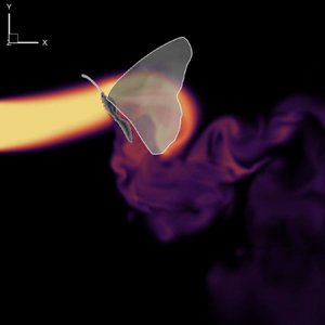
Notably, at the end of the downstroke (t/T = 7.625), the deceleration causes tremendous deformation at the wing tips due to the inertial forces. Such strong end-stop motion triggers forwards movement in the nearby airflow. Immediately following the end-stop motion, the upstroke begins. This rapid change in the wing flapping direction forms a lower pressure region on the wings’ lower surface inducing a forwards and upwards airflow. This induced flow eventually moves towards the region near antennae. The resultant upwards-going eddies remain observable in the downwash region at the beginning of the subsequent downstroke (t/T = 7.125).

In addition to the LEV around the flapping wing, a vortex formation near the antenna is observed. The coupled wing–body oscillation motion during the flapping cycle potentially promotes the strength of the vortex formation on the antenna. We visualize the vortex along the antennae (figure 11a) and compute the absolute non-dimensional circulation $(|{\varGamma ^\ast }|)$ of the antenna vortex at different time instants. As shown in figure 11(b), the vortex around the antenna root appears to have the strongest strength, and its strength almost linearly decreases along the antenna. To explore the development of the antenna vortex, figure 11(c) shows the time course of the antenna vortex circulation at 20 % antenna length L_a from the base. The circulation of antenna vortex increases during the downstroke and decreases during the upstroke. This observation indicates that the formation of antennae vortices is strongly affected by the flapping wing motion. Since the formation of the vortex can affect the local flow distribution around the antenna, we suspect such a wing–antenna interaction potentially impacts the odour perception of insects in an odour-tracking flight.

Figure 11.

(a) Contour slicecut of the antenna vortex (AV) at t/T = 7.625, coloured by antennae-wise vorticity; (b) non-dimensional AV circulation $|{\varGamma ^\mathrm{\ast }}|$ along one antenna. (c) Time history of non-dimensional AV circulation $|{\varGamma ^\mathrm{\ast }}|$ at 20 % l_a/L_a, the l_a is the distance from the slide cut to antenna root and L_a is the length of the antenna. See the supplementary movie 2.

To evaluate how the vortex formation near the antenna impacts the odour perception of the butterfly, the odour intensity along the antenna is obtained by solving the advection-diffusion equation at each time step. During the simulation, eight probes along the antennae (figure 12a) were set to collect the odour intensity data over eight flapping cycles. Figure 12(b) shows the time history of the normalized odour intensity according to the probe locations. At the first flapping cycle, the odour intensity is not stable because the odour has just been released from the odour source and has not reached the antenna yet. After approximately two flapping cycles, we observe periodical patterns of odour intensity. The overall odour intensity trend syncs with the frequency of the flapping wing. The odour intensity reaches its maximum value during the wing reversals when the wings move close to the antennae. The minimum value of odour intensity appears near the middle downstrokes. The changing trend of odour intensity during each flapping cycle is aligned well with the time history of antenna vortex circulation (figure 11c). The formation of antenna vortices creates a local whirlpool and serves as an odour sink to draw more odour-plume particles to its antenna. This observation is similar to the odour mass flux data reported in a previous fruit fly study (Li et al. Reference Li, Dong and Zhao2018). Unlike fruit flies, butterflies have horizontal-oriented long antennae. Our results indicate that the odour intensity at different locations along the antenna presents different variation magnitudes and peak durations. For instance, the probes near the head (i.e. probes 1–4) show a smaller peak-to-peak variation of odour intensity but a more extended peak period. The probes near the outer position of the antenna (i.e. probes 5–8) present larger peak-to-peak variation, but a shorter peak period. This difference can lead to a spatial variation of odour intensity along the antennae. As shown in figure 12(c), the spatial distribution of odour intensity presents a significant gradient along the antenna for both downstroke and upstroke. In conjunction with figure 11(b), we can see that the changing trend of odour intensity along the antenna is similar to the antenna vortex circulation (highest at the base and gradually decreasing to the antenna tip). For navigating an odour landscape in nature, one of the most significant challenges is to determine the distance and orientation towards the odour source. To perceive the precise location of the odour source, insects must integrate odour information across both space and time (Pannunzi & Nowotny Reference Pannunzi and Nowotny2019). The authors suspect that the odour intensity gradient along the antenna can enhance the capability of flying butterflies to determine the direction of the odour source and potentially contribute to the stereo-olfaction of insects in odour-guided navigation.

Figure 12.

(a) Probe locations for measuring the odour intensity. (b) Odour intensity distribution along the antenna at selected instants, t/T = 7.0, 7.25, 7.5 and 7.75. (c) Time history of normalized odour intensity (C/C ₀) at the corresponding probes.

To examine the odour concentration field, we visualized odour plume structures coloured by the normalized odour intensity (C/C ₀) (figure 13). In our simulation set-up, a uniform odour was released upstream in the numerical wind tunnel. As the odourant-laden airflow passes through the butterfly, the flapping wings create a strong wing-induced flow and push the odour upwards. This phenomenon corresponds to the observation (figure 10) that the flapping motion directs the flow towards the region near the antennae. Consequently, this induced flow enhances odour sensory perception by extending the odour sampling range in the vertical direction.

Figure 13.

Contour of odour intensity C/C ₀ at t/T = 7.125, 7.375, 7.625 and 7.875. The three columns represent the top view, the side view and the perspective view, respectively. For the top view, the contour slice is cut at the middle bottom plane to demonstrate the odour concentration in the far field. For the side view, the slice is cut laterally in the middle. For perspective view, two additional slices are cut near the wing root. See the supplementary movie 3.

Figure 14 shows the surface distribution of cycle-averaged odour intensity on both the dorsal and ventral sides. The cycle-averaged odour intensity is projected onto a template model featuring planar wings. Our findings reveal that a significant concentration of odour accumulates around the antenna root and the head during forwards flight. This suggests that the antennae are strategically positioned to receive odour stimuli while minimizing air disturbance compared with other locations along the body. In addition to the body, the top surface of the hindwing comes into contact with more odourants than other parts of the wings. This finding suggests the feasibility of incorporating odour sensors on the top of the hindwing for manmade designs such as micro aerial vehicles (MAVs) if required.

Figure 14.

Distribution of the cycle averaged odour intensity C/C ₀ on the surface of the wings and the body.

3.2. Effects of wing-induced flow on olfaction

To evaluate how the wing-induced flow impacts the odourant transportation, we simulated a body-only case for comparison. The body-only case is modified from the baseline case by removing the flapping wings while maintaining all other settings the same. Figure 15 shows the comparison of the instantaneous lift and drag forces between the baseline case and the body-only case. Due to the wing–body interaction, the cycle-averaged lift coefficient ${\bar{C}_L}$ generated by the body is increased from 1.07 (body only) to 8.35 (baseline). Meanwhile, the cycle-averaged drag coefficient ${\bar{C}_D}$ is also increased from 0.10 (body only) to 0.29 (baseline).

Figure 15.

Time history of the (a) lift coefficient ${C_L}$ and (b) drag coefficient ${C_D}$ of the body in the baseline and body-only case.

In addition to the influence on the overall aerodynamic forces, the wing-induced flow is expected to have an impact on the odourant transport around antennae, and thus affect the olfactory function. We first compare the formation of antennae vortices between the baseline case and the body-only case at an instant during the wing reversal (figure 16a,b). Based on the contours, the antennae vortices are significantly enhanced by the flapping-wing motion. From figure 16(c), we can see that the antenna vortex circulation of the baseline model is greater than that of the body-only model along the antenna. The wing-induced flow enhanced the average antenna vortex circulation by 2.78 times compared with the body-only case. In addition, the wing–antenna interaction also creates a spatial variation of antenna vortex circulation along the antenna. Without the flapping wings, the circulation values remain relatively constant along the antenna. Moreover, we calculated the time history of circulation at l_a/L_a = 0.2 in figure 16(d), and we found that the wing-induced flow makes the antenna vortex circulation vary along the time course. Due to the body oscillation motion, the antenna vortex circulation of the body-only model also presents slight temporal variation during the flapping cycle, but its peak value is much lower than the baseline case. By comparing the antenna vortex circulation between the two cases, the first peak of antenna vortex circulation for the baseline case (red curve) is due to the body pitching motion, while the second peak (primary peak) is due to the wing-induced flow. For the whole cycle, the cycle-averaged antenna vortex circulation $|{\overline {{\varGamma^\ast }} } |$ of the body-only case is only 43 % of the baseline case.

Figure 16.

Contour slicecut of the antenna vortex (AV) at t/T = 7.625, coloured by antennae-wise vorticity: (a) baseline case and (b) body-only case; (c) non-dimensional AV circulation $|{\varGamma ^\mathrm{\ast }}|$ along the antenna. (d) Time history of non-dimensional AV circulation $|{\varGamma ^\mathrm{\ast }}|$ at 20 % l_a/L_a.

The effect of wing-induced flow on antenna vortex can affect the odour intensity along the antennae. Figure 17 compares the odour intensity (C/C ₀) between the baseline case and the body-only case. In the body-only case, the temporal fluctuations of odour intensity along the antennae are less pronounced compared with the baseline case. Except for probe 1, the odour intensity at all other probes in the baseline case fluctuates significantly more than in the body-only case. To quantify this fluctuation, we calculate the odour gradient $(\boldsymbol{\nabla }C/{C_0})$ by dividing the change of C/C ₀ between two adjacent probes by their distance along the antenna (figure 18a). Since the odour gradients vary with time, we then calculate the odour gradient along 13 evenly distributed time instants. In figure 18(b), we plot the odour gradient overtime at four probe locations. The gradient of the body-only model remains nearly zero while the baseline model has a much larger variation during the flapping cycle. Previous experimental studies indicated insects show a better response rate to pulsatile odour stimuli than uniformly distributed odours (Daly et al. Reference Daly, Kalwar, Hatfield, Staudacher and Bradley2013). The tiny temporal variation of odour intensity for the body-only model (figure 18b) may make the nervous system of the butterfly less sensitive to the odour information, which can potentially cause olfactory adaptation (or sensory fatigue). From our results, the wing-induced flow can amplify the temporal variation of the odour intensity in flight, which will increase the firing rate of the chemoreceptors on antennae and potentially prevent the olfactory adaptation.

Figure 17.

(a,b) Probe locations for measuring the odour intensity. (c) Comparison of odour intensity C/C ₀ between the baseline case (with flapping wings) and the body-only case (without flapping wings) at probe locations 1, 3, 6, 8.

Figure 18.

(a) Definition of the odour gradient ∇C/C ₀ along the antenna at a selected instant. (b) Comparison of the time history of the odour gradient between the baseline case (with flapping wings, solid symbol) and the body-only case (without flapping wings, empty symbol) at probe locations 1, 3, 6, 8 as labelled in figure 17. The data are fitted using a six-term polynomial trendline.

Figure 19 compares the odour intensity contour between the baseline case and the body-only case. In the body-only case, without the wing-induced flow, the upstream-released odour may not reach the butterfly's antennae. However, in the baseline case, the wing-induced flow pushes the odour plume upwards, ensuring better coverage of the odour plume over the antennae compared with the body-only case. This improved coverage may increase the overall intensity of the odour concentration on the antennae. Just as shown in figure 17, under the current simulation set-up, the wing-induced flow can enhance the cycle-averaged odour intensity by up to 14.29 times. This largest difference between the two cases occurs at the antennae root. In the baseline case, the root immerses at the plume centre where the odour intensity is the highest, causing a significant difference compared with the body-only case, where the antennae root misses the odour plume. Thus, these observations suggest that the wing-induced flow can provide the butterfly with a better odour-sampling ability.

Figure 19.

The lateral-centre contour of odour intensity C/C ₀ for (a) the baseline case and (c) the body-only case at t/T = 7.625.

The distribution of the cycle-averaged odour intensity shows how the body contacts the odourants (figure 20). In the body-only case, the most intense odour is distributed on the abdomen which is significantly different from what we observed in the baseline case. This observation proves our hypothesis that the wing-induced flow can enhance the olfactory function of flying insects. The antenna of the butterfly has a lateral pointing pair of antennae which can help the lateral odour sampling.

Figure 20.

Distribution of the cycle-averaged odour intensity C/C ₀ for the baseline case (left) and the body-only case (right).

Despite the results, some limitations must be acknowledged. Our observations regarding the enhancement of peak or cycle-averaged odour intensity through wing-induced flow are derived from a simulation set-up with a fixed odour source location, which is slightly lower than the butterfly. In this set-up, the wing-induced flow exhibits an exceptional ability to draw the odour plume upwards, thereby improving odour sampling. We observed enhanced peak or cycle-averaged odour intensity, but this enhanced peak odour intensity may simply be a byproduct of this improved odour sampling. Thus, if the wing-induced flow fails to direct the odour plume through the antennae, such as when the odour source is positioned much lower or upper than our set-up, the peak odour intensity would not be amplified. Therefore, our observation of the enhancement of overall odour intensity may not apply to all other scenarios.

3.3. Effects of inter-antennal angle

Observations show that antennal movements are an important part of the active odour sensing of insects (Claverie et al. Reference Claverie, Steinmann, Bandjee, Buvat and Casas2022). These movements are made possible by muscles near the antenna joints, allowing insects to adjust their antennae to optimize odour stimuli. For example, a butterfly may oscillate its antennae while perched on a flower (Scott Reference Scott1986). Such oscillations help the butterfly improve odour stimuli because it is immersed in a strong odour field which can cause odour sensory fatigue. However, in a forwards flight, the antennae of the butterfly remain fixed to the head based on our observation and other studies (Krishnan et al. Reference Krishnan, Prabhakar, Sudarsan and Sane2012). Although antennae positions are fixed, we observed that each butterfly maintains distinct antenna positions, which may affect the performance of aerodynamics or odour sensory abilities. To investigate the impacts of inter-antennal positions, this section compared the baseline model with those with different antennae positions under the same flow conditions. The distinct distance among these cases could give deeper insight into the wing–antennae interaction mechanism. The inter-antennal angle (α) between antennae is defined in figure 21. We hypothesize that different α values can affect the butterfly's horizontal odour sampling range and the odour intensity along the antennae. In this section, we present the results of simulations for four additional values of α (130°, 105°, 55° and 30°) under the same flow conditions as the baseline case, which corresponds to an inter-antennal angle of 80° (baseline case).

Figure 21.

Definition of inter-antennal angle α. The angle is measured by connecting two antenna tips and the centre of two antenna root joints.

To evaluate the impact of inter-antennal angle on the wing–antenna interaction, figure 22 compares the formation of antennae vortices when the odour intensity reaches its peak for each case (t/T = 7.625). At α = 130°, the antennae vortices are uniformly developed along the antenna from root to tip. As the inter-antennal angle gradually decreases to 30°, the antennae vortices are still strong near the antenna root, while its strength significantly decreases close to the antenna tip since it has the largest distance from the flapping wings. Figure 23 demonstrates the variation of antenna vortex circulations along the antenna for each case. In general, antenna vortex circulation decreases along the antenna from root to tip. Notably, when α is 130°, the antennae vortices near antennae tips are unusually strong, likely due to the entangling of antennae vortices and leading-edge vortices in the presence of the flapping wing. As the inter-antennal angle α decreases from 130° to 30°, the distance between flapping wings and antennae is enlarged. As a consequence, the circulation of antennae vortices also decreases. However, the enhanced antennae vortices for larger inter-antennal angle cases (130° and 105°) present smaller gradients along the antennae. The cases with smaller inter-antennal angles (55° and 30°), however, have larger variations from antenna root to tip. This result suggests that smaller α values can provide a larger circulation gradient along the antennae.

Figure 22.

Contour of slice cuts of AVs (coloured by antennae-wise vorticity) at t/T = 7.625 for α = (a) 130°, (b) 105°, (c) 80°, (d) 55° and (e) 30°.

Figure 23.

Antenna vortex circulation along one antenna at t/T = 7.625 for α = 130°, 105°, 80°, 55° and 30°.

Moreover, given the demonstrated amplification effects of wing-induced flow on odour intensity, we hypothesize that the effects of α on the wing-induced circulation of antenna vortex could also influence the odour intensity distribution on the antennae. In figure 24(c), we present the time history of odour intensity (C/C ₀) at probe locations labelled in figure 24(a). As α decreases, the variation amplitude of the curve increases, with peak odour intensity decreasing closer to the tip and valley odour intensity increasing closer to the root. This result suggests that smaller α values can provide a larger odour intensity varying rate that is caused by wing motions, potentially increasing the sensitivity of odour tracking by avoiding the odour sensory fatigue. For example, at α = 130°, the difference between the highest and the lowest values of red curve during the periodical stage (figure 24c), at probe location 1, is less than 0.1. For the same probe location, the peak-to-peak value for the α = 30° case is approximately 0.4.

Figure 24.

(a) Probe locations for measuring the odour intensity. (b) Illustration of five inter-antennal angles. (c) Time history of normalized odour intensity C/C ₀ for α = 130°, 105°, 80°, 55° and 30°.

Despite the odour sensory benefits of smaller α values, extremely narrow inter-antennal angles are not commonly observed in natural butterflies. One explanation for this could be that the inter-antennal angle of the antennae is related to the horizontal odour sampling range. To investigate this hypothesis, we calculated the effective sampling range by tracing back the trajectories of the collected odour particles to the odour source, where the collected particles are defined as those that successfully reach the antennae. Figure 25 illustrates this process, and the resulting odour sampling range maps for five different values of α ranging from 130° to 30° are shown in figure 26. As expected, smaller α values yield a more restricted horizontal range of odour sampling. By comparing the odour sampling range of butterfly antennae at different inter-antennal angles, we suspect that the inter-antennal angle is not arbitrary during flight. Instead, it appears to be within a specific range that represents a trade-off between preventing sensory fatigue and odour sampling range.

Figure 25.

Trajectory of the collected particles following the streamlines from antennae to the odour source. The red contour represents a surface slice cut on YZ plane near the odour source.

Figure 26.

Odour sampling range maps with varying inter-antennal angles for α = (a) 130°, (b) 105°, (c) 80°, (d) 55° and (e) 30°.

3.4. Effects of wing flexibility

Wing flexibility is another key factor affecting unsteady airflow field and associated odourant distribution. Many studies have indicated that flexible wings can achieve better aerodynamic performance than rigid wings (Zheng et al. Reference Zheng, Hedrick and Mittal2013; Johansson & Henningsson Reference Johansson and Henningsson2021), but it is unclear how wing flexibility impacts the odour-tracking ability of insects. As described in § 2.2, we created rigid wings planforms based on the baseline wings. In figure 27(a,b), we first compare the instantaneous lift and drag coefficient between the baseline case and the rigid wing. The cycle-averaged lift coefficient ${\bar{C}_L}$ of the rigid wing (6.47) is 7.5 % larger than that of the baseline wing (6.02). The cycle-averaged drag coefficient ${\bar{C}_D}$ is increased from −4.63 × 10⁻⁴ (baseline) to 1.00 (rigid wing).

Figure 27.

Time history of (a) lift coefficient ${C_L}$, (b) drag coefficient ${C_D}$ and (c) power coefficient $C_{pw,mech}^{0\,\%}$ of wings in the baseline and rigid-wing case.

The mechanical power coefficient of the rigid wing is calculated by (2.11) which does not consider elastic energy storage. Figure 27(c) shows the time history of these two mechanical power coefficients $C_{pw,mech}^{0\,\%}$ of the baseline case and the rigid-wing case. As summarized in table 3, the rigid-wing model exhibits a power consumption of 32.83 $(C_{pw,mech}^{0\,\%})$ representing a 22.37 % increase compared with the baseline model. However, the lift-to-power ratio of the rigid wing is 9.09 % lower than that in the baseline case.

Table 3.

Aerodynamics performance comparison of the baseline case with the rigid-wing case.

Although flexible wings generate less lift than rigid wings, the overall power efficiency for lift generation is significantly higher due to the high power consumption. This finding aligns with a previous butterfly study, which reported that three rigid-wing cases exhibited 30 % to 50 % less lift-to-power ratio than the flexible-wing case (Zheng et al. Reference Zheng, Hedrick and Mittal2013). It is worth noting that the reduction observed by Zheng et al. is greater than our result, likely attributed to differences in modelling rigid wings. In their model, rigid wings generate less lift than flexible wings while consuming a similar amount of power as in our model. Consequently, the combination of reduced lift and equal power consumption results in an even larger lift-to-power ratio.

Figure 28(a) presents the cycle-averaged lift and aerodynamic power coefficient distributions of the rigid wing. Compared with the flexible wing model (baseline case in figure 9), the rigid wing model shows a more extensive lift contour region near the wing leading-edge and a larger aerodynamic power contour region near the wingtip. The difference of the lift generation and aerodynamic power consumptions between the rigid wing and flexible wing is shown in figure 28(b). In general, the rigid wing generates less lift near the wingtip region along the leading-edge, while gains more lift close to the trailing-edge portion of the forewing. Due to the modification of the hindwing wing pitch angles when the rigid wing model is created, the hindwing of the rigid wing model generates more lift than the baseline model. As expected, the tip region of the rigid wing model consumes a significant amount more of aerodynamic power than the flexible wing. Because the tip region of the butterfly wing presents more deformation during flapping, it prevents the formation of a strong tip vortex. It thus reduces power consumption and leads to a better power efficiency for flexible wings (baseline case).

Figure 28.

(a) Wing surface distribution of cycle-averaged lift coefficient ${\bar{C}_L}$ and aerodynamic power coefficient $({\bar{C}_{pw,aero}})$ in the rigid wing case. (b) Difference of cycle-averaged lift coefficient $(\Delta {\bar{C}_L})$ and aerodynamic power coefficient $(\Delta {\bar{C}_{pw,aero}})$ between the rigid wing case and the baseline case. In (b), the red colour regions indicate the value of rigid wing is higher than the baseline case.

The effects of wing flexibility on olfactory function are also evaluated by comparing the odour intensity on antennae (figure 29). We collected the data at the probes along the antennae in the same manner as the baseline case. From the time history of the odour intensity at all four probe locations, the amplitude of the baseline case is larger than the rigid wing case. The flexible wings create a higher peak to peak value of odour intensity than the rigid wings by up to 24 %. Experimental studies have shown that many insects respond better to pulsatile odour stimuli (Baker et al. Reference Baker, Willis, Haynes, Phelan, Haynes, Phelan, Haynes and Phelan1985; Daly et al. Reference Daly, Kalwar, Hatfield, Staudacher and Bradley2013). The higher variation magnitude of odour intensity caused by the flexible wings thus potentially increases the chance of detecting the odour source in flight. The odour plume structure is visualized in figure 30 and coloured by the normalized odour intensity C/C ₀. Both the baseline case and rigid wing case can push the incoming odour stream upwards. Despite the local odour intensity difference near the antennae, the overall odour concentration fields are roughly identical except for the far field.

Figure 29.

Comparison of time history of normalized odour intensity between the baseline and rigid wing case at probe locations 1, 3, 6, 8 as labelled in figure 12.

Figure 30.

The lateral-centre contour of normalized odour intensity for (a) the baseline and (b) the rigid wing case.

3.5. Effects of thorax pitching

To examine the effects of body oscillation, we operated additional fixed-thorax cases for the models with fixed thorax pitch angles θ_t. Figure 5(b) shows that the butterfly thorax pitch dynamically from 27.32° to 60.82° during each flapping cycle. In this section, we run four additional simulations with constant θ_t of 30°, 40°, 50° and 60° while maintaining all other settings the same as the baseline case. Since the wings are attached to the thorax, the simulations with a fixed thorax pitch angle will also eliminate the stroke plan variation during the flapping cycle. In addition, the motion of the antennae will also be removed because it stays rigidly attached to the head. However, the abdomen is still undulating with the same kinematics during the flight to avoid introducing other influence factors on the unsteady flow field.

Figures 31(a) and 31(b) show the time history of the drag and lift. For the fixed thorax angles of the 50° and 60° cases, lift forces are positive throughout the entire flapping cycle. However, these models cannot produce sufficient thrust to overcome the fluid drag along the horizontal direction. The cases with fixed thorax angles of 30° and 40° cases can generate thrust to achieve a forwards flight, but they cannot generate sufficient lift force in the vertical direction to balance its body weight.

Figure 31.

Time history of (a) lift coefficient ${C_L}$ and (b) drag coefficient ${C_D}$ on the wing between baseline case and fixed thorax cases. (c) Time history of mechanical power coefficient $C_{pw,mech}^{100\,\%}$ which has 100 % elastic storage. (d) Time history of mechanical power coefficient $C_{pw,mech}^{0\,\%}$ which has 0 % elastic storage. The actual mechanical power lies in between the two curves. The grey-shaded area represents the downstroke period.

Figures 31(c) and 31(d) compares the mechanical power of the stationary thorax cases with the baseline case. By comparing the negative mechanical power between baseline case and other cases, we found that the thorax pitching motion only saves a small amount of power in the form of energy storage. The majority contribution of the energy storage is due to elastic deformation. The cycle-averaged mechanical power coefficient and lift-to-power ratio are summarized in table 4, where the percentages represent the increment or reduction with respect to the baseline case. Our simulation results indicate that, with the same flapping kinematics, the dynamic thorax pitching motion can improve power efficiency by 10 % to 50 % compared with the case with a stationary thorax pitch angle.

Table 4.

Aerodynamics performance comparison among the baseline case and fixed-thorax cases.

To address the effects of thorax pitching on the odour sensory of the antennae, we compare the odour intensity of the cases with fixed thorax angles with the baseline case. Since the overall variation trend of odour intensity at each probe location is similar, only the odour intensity of probe 8 is selected to plot in figure 32. Comparing with the baseline case, the curves of the four stationary thorax cases have smaller amplitudes. As a result, the baseline case exhibits a steeper slope increase in odour intensity over time compared with all stationary thorax cases. Thus, the odour intensity slope of the baseline case is steeper than all stationary thorax cases. Such higher slopes represent faster varying rate of the odour intensity on the antennae, which could potentially prevent the potential of olfactory adaptation. We speculate that the thorax motion during the surging upwind flight may achieve a similar function as the antennal oscillation when the insects land on the odour source. Previous experimental observations have illustrated that insects oscillate antennae frequently, even when not in flight. A study of bumble bees found that such antennal scanning movements are actively involved in odour sensory, and the antennal oscillating can increase the odour sampling rate by up to 200 % (Claverie et al. Reference Claverie, Steinmann, Bandjee, Buvat and Casas2022). In butterfly flight, the thorax oscillation can cause the oscillating movement of the antennae. Such a motion can amplify the odour intensity along the antennae and thus potentially benefit odour detection in flight.

Figure 32.

Time history of normalized odour intensity of the baseline case and the fixed-thorax cases at probe 8.

Figure 33 compares the odour concentration field between butterfly models with different fixed thorax pitching angles. Due to the body posture at different thorax pitching angles, the overall odour concentration distributions are very different in both near and far fields. In conjunction with figure 13, the dynamic thorax pitching motion can potentially increase the odour sampling range and create pulsatile odour stimuli near its antennae.

Figure 33.

The lateral-centre contour of normalized odour intensity C/C ₀ for fixed-thorax cases as θ_t = (a) 30°, (b) 40°, (c) 50° and (d) 60°.

3.6. Antenna vortex formation and odour perception in gliding flight

Previously, our comparison between the baseline case and the body-only case revealed that the flapping wing creates an odour gradient along the antennae and temporal variations in odour intensity. Although the body-only case comparison helps isolate the wing's effects, the mere presence of the wing may still influence the outcomes. To bolster the robustness of our observations and conclusions, we expanded our investigation to include a gliding flight case, considering that butterflies are adept gliders (Shyy et al. Reference Shyy, Lian, Tang, Viieru and Liu2007; Park et al. Reference Park, Bae, Lee, Jeon and Choi2010; Gibo & Pallett Reference Gibo and Pallett1979).

In this section, the model in the gliding case remains stationary, extracted from the baseline model at t/T = 0.45. By the 8th cycle, the gliding case reaches a steady state, with a lift coefficient on one wing of 0.90, accounting for 14.95 % of the baseline case. The drag coefficient on one wing is 0.66, indicating a lift-to-drag ratio of 1.36, which is within a reasonable range compared with that reported in another study of the swallowtail butterfly (Park et al. Reference Park, Bae, Lee, Jeon and Choi2010). The aerodynamic power coefficient is 0.39, representing 1.35 % of the baseline case. In addition, the total lift that is generated by the whole butterfly is 0.93 mN, which supports 16.04 % of the total weight, 5.83 mN. This low weight supporting performance is due to the insufficient flight speed. Since this gliding model is used to investigate if the mere presence of the wing influences the odour perception, we intentionally keep the flight speed the same as the baseline case.

Figures 34(a) and 34(b) compare the antenna vortices distribution along antennae between the baseline case and the gliding flight case, while figure 34(c) compares the circulation between two cases. The baseline case exhibits a larger magnitude of circulation compared with the gliding case; importantly, the distribution of circulation along the antennae remains relatively constant. Analysing the temporal variation in figure 34(d), the gliding case shows constant circulation at 20 % l_a/L_a over time indicating a steady state.

Figure 34.

Contour slicecut of the antenna vortex (AV) at t/T = 7.45, coloured by antennae-wise vorticity: (a) baseline case and (b) gliding flight case; (c) non-dimensional AV circulation $|{\varGamma ^\mathrm{\ast }}|$ along the antenna. (d) Time history of non-dimensional AV circulation $|{\varGamma ^\mathrm{\ast }}|$ at 20 % l_a/L_a.

Figure 35 presents a comparison of the time history of odour intensity at four probes specifically employed for the body-only comparison. As the simulation achieves a steady state by the 8th cycle, the odour intensity in the gliding flight case inevitably remains constant. Notably, it is important to highlight that proximity to the head corresponds to stronger odour intensity, while closer proximity to the antennae tip results in lower odour intensity. This discrepancy may arise from the smaller sampling range in the gliding flight case compared with the baseline case. The gliding flight case exhibits a reduced vertical sampling range due to the fixed thorax pitching angle, preventing the upwards induction of the odour plume. This observation is further illustrated in figure 36(b), where the odour plume, upon reaching the butterfly, ceases to be induced upwards, unlike in the baseline case where flapping wings can propel the odourant in an upwards direction.

Figure 35.

Comparison of C/C ₀ time history between the baseline and gliding flight case at probe locations 1, 3, 6, 8.

Figure 36.

Lateral-centre contour of normalized odour intensity for (a) the baseline and (b) the gliding flight case.

3.7. Wing–antenna interaction: mechanism of odour fatigue resistance

Flapping wings, a defining trait of flying insects, have received significant interest among scientists for their potential advantages over conventional propulsion methods, especially at low Reynolds numbers. This curiosity has led to a comprehensive exploration and identification of multiple performance-enhancing mechanisms within the scientific literature. Key among these is the fundamental mechanism of insect flight, which includes phenomena such as delayed stall, wake capture and rotational circulation (Dickinson, Lehmann & Sane Reference Dickinson, Lehmann and Sane1999). Such mechanisms have been pivotal in advancing our understanding of unsteady aerodynamics and lift generation in these creatures. Further, the literature meticulously documents the enhancements attributed to various interactive mechanisms, as summarized in table 5. These mechanisms encompass interactions between wings, as well as between wings and wakes, the effects of wing flexibility, and the dynamics between wings and the insect body. The primary focus of these studies has been to understand how these interactions contribute to aerodynamic performance, particularly in terms of lift generation and power efficiency.

Table 5.

Performance enhancement mechanisms in insect flight.

Building upon this foundation, our current research has uncovered a novel interactive mechanism that links the flapping motion of wings with the function of antennae, thereby augmenting odour perception. This interaction significantly contributes to preventing odour fatigue and expanding the range of odour sampling during odour-guided flapping flight. This discovery not only enriches our comprehension of insect flight dynamics but also opens new avenues for understanding how flying insects interact with their environment through enhanced olfactory detection.

Our observations indicate that the wing flapping motion generates beneficial disturbances in the incoming flow, redirecting the odour plume towards the antennae and inducing fluctuations in odour intensity over the antennae. This phenomenon is caused by the wing–antennae interaction, where flapping wing motion produces pulsatile-induced flow directed towards the antennae. Meanwhile, the circulation of antenna vortex flatulates due to the pulsatile induced flow, resulting in fluctuations in odour intensity near the antennae. In our numerical simulations of free flying butterfly, the amplitude of odour intensity fluctuation (peak-to-valley of C/C ₀) reaches up to 0.84 at antenna tip (probe 8), whereas it diminishes to 0.1 without the assistance of flapping wing motion, indicating an approximately 8.4 times enhancement in odour fluctuation. At this probe location, the contribution of the wing–antenna interaction to the odour fatigue resistance is 88.10 %. While the magnitude of this enhancement varies depending on the location of the measurement over the antennae, it is consistently present along the antennae, with the highest enhancement observed at the antennae tip. The odour fatigue resistance of insects relies on these fluctuations that are generated by the wing–antennae interaction.

The strength of odour fatigue resistance can be adjusted for the different flight purposes by modifying the inter-antennal angle. A larger inter-antennal angle weakens the wing effect on odour fluctuation but provides a larger odour sampling range. In contrast, a lower inter-antennal angle results in stronger fluctuations induced by wing motion but restricts the odour sampling range. The trade-offs between odour fatigue resistance and odour sampling enable butterflies to have a broader sampling range when farther from the odour source and better odour fatigue resistance when closer to the target. For example, as insects approach the target, where they need both visual and olfactory cues (Saxena, Natesan & Sane Reference Saxena, Natesan and Sane2018), overcoming odour fatigue due to the strong odour concentration field becomes important. Hence, at close range to the odour source, a smaller inter-antennal angle is preferable for enhanced odour fatigue resistance. In contrast, at farther distances from the odour source, a larger inter-antennal angle is advantageous due to the need for broader sampling range. The lager inter-antennal angle trades odour fatigue resistance for a broader odour sampling range. These results indicate the possibility that, by changing the inter-antennal angle, insects can balance the odour sampling range and odour fatigue resistance, which can also provide insights for the bio-inspired MAV designs.

In terms of the effect of thorax pitching motion and wing flexibility, they contribute to the generation of odour intensity fluctuation over antennae. However, their effects are limited comparing with the effects of wing-antenna interaction. The amplitude of odour intensity fluctuation in the rigid-wing case is up to 0.75 at probe 8, which is 89.29 % of the baseline case, indicating that the wing flexibility contributes only up to 10.71 % to the generation of the fluctuation. When comparing our simulated fixed-thorax cases with the baseline case at probe 8, thorax pitching motion contributes from 2.8 % to 22.56 % to the odour intensity fluctuation. In contrast to the contribution of wing–antenna interaction, which is 88.10 %, the contribution of wing flexibility and thorax-pitching motion to the odour fatigue resistance is relatively low. The percentages reported represent the relative contributions of wing flexibility and thorax pitching motion to odour intensity fluctuation at the peak value of each case. It is important to note that these peak-to-valley values may occur at different phases across the cases, preventing them from being summed to 100 %. Thus, they should be interpreted independently as relative measures of contribution.

While our findings contribute insights into the butterfly's ability to prevent odour fatigue through wing–antenna interaction, it is important to acknowledge several limitations that may affect the interpretation of the results. The simulations were based on a fixed odour source location slightly below the butterfly. In nature, depending on the odour-tracking mode of the butterfly, it may fly above or below the odour source. Therefore, the strength of the wing-induced effect on odour fluctuation may vary with the relative position between the butterfly and the odour source. Additionally, the location of the odour source can also influence the butterfly's flight behaviour. For instance, when the antennae are outside the odour plume, the butterfly may switch from an upwind surging flight to another odour-tracking flight mode, such as zigzagging flight, which may involve wing and body kinematics different from those studied here. In such cases, the enhancement of odour sampling range becomes more important than preventing odour fatigue, a factor not supported by our reported data and beyond the scope of our current study. The complexity introduced by the variability in odour source location suggests several avenues for future research. Future studies could explore how varying odour source positions affect the butterfly's ability to prevent odour fatigue and how this variability may influence the butterfly's odour-tracking behaviour.

4. Conclusions

In this study, we conducted numerical simulations to investigate the unsteady aerodynamics and olfactory performance of a monarch butterfly during an upwind surge flight, using an in-house CFD solver. Our results reveal that the interaction between wing flapping motion and antennae generates significant fluctuations in odour intensity along the antennae. Specifically, under our simulation set-up, the amplitude of these fluctuations is enhanced by up to 8.4 times due to wing–antenna interaction. While other flight features, such as wing flexibility and thorax pitching, also contribute to odour fluctuation, their impact is considerably less pronounced compared with the dominant influence of the wing–antenna interaction. We found that the wing-induced flow resulting from the wing–antenna interaction accounts for up to 88.10 % of the odour fluctuation, making it the primary contributor. This fluctuation plays a crucial role in preventing insects from experiencing odour fatigue, particularly in highly concentrated odour fields. Furthermore, our study highlights the trade-off between odour fatigue resistance and odour sampling range, with smaller inter-antennal angles prioritizing odour fatigue resistance and larger angles sacrificing resistance for broader sampling range. These findings provide valuable insights into the adaptive strategies of flying insects and have potential applications for bio-inspired designs like odour detection MAVs.

Supplemental movies

Supplementary movies are available at https://doi.org/10.1017/jfm.2024.644.

Acknowledgements

This research was supported by the National Science Foundation (CBET-2042368) monitored by Dr R.D. Joslin and Air Force Office of Scientific Research (FA9550-24-1-0122) monitored by Dr P. Bradshaw.

Declaration of interests

The authors report no conflict of interest.

Data availability

The reconstructed kinematics and CFD simulation results of this study are available upon reasonable request.

References

Allers, M., Ahrens, A., Hitzemann, M., Bock, H., Wolf, T., Radunz, J., Meyer, F., Wilsenack, F., Zimmermann, S. & Ficks, A. 2023 Real-time remote detection of airborne chemical hazards - an unmanned aerial vehicle (UAV) carrying an Ion mobility spectrometer. IEEE Sens. J. 23 (15), 16562–16570.CrossRef Google Scholar

Aono, H. & Liu, H. 2006 Vortical structure and aerodynamics of Hawkmoth Hovering. J. Biomech. Sci. Engng 1 (1), 234–245.CrossRef Google Scholar

Ashley, H. & Rodden, W.P. 1972 Wing-body aerodynamic interaction. Annu. Rev. Fluid Mech. 4 (1), 431–472.CrossRef Google Scholar

Baker, K.L., Dickinson, M., Findley, T.M., Gire, D.H., Louis, M., Suver, M.P., Verhagen, J.V., Nagel, K.I. & Smear, M.C. 2018 Algorithms for olfactory search across species. J. Neurosci. 38 (44), 9383–9389.CrossRef Google Scholar PubMed

Baker, T.C. 1989 Pheromones and flight behavior. In Insect Flight, pp. 231–255. CRC.CrossRef Google Scholar

Baker, T.C., Willis, M.A., Haynes, K.F., Phelan, P.L., Haynes, F., Phelan, P.L., Haynes, K.F. & Phelan, P.L. 1985 A pulsed cloud of sex pheromone elicits upwind flight in male moths. Physiol. Entomol. 10 (3), 257–265.CrossRef Google Scholar

Betts, C.R. & Wootton, R.J. 1988 Wing shape and flight behaviour in butterflies (Lepidoptera: Papilionoidea and Hesperioidea): a preliminary analysis. J. Expl Biol. 138 (1), 271–288.CrossRef Google Scholar

Bode-Oke, A.T. & Dong, H. 2020 The reverse flight of a monarch butterfly (Danaus plexippus) is characterized by a weight-supporting upstroke and postural changes. J. R. Soc. Interface 17 (167), 20200268.CrossRef Google Scholar PubMed

Chang, S., Lai, Y., Lin, Y. & Yang, J. 2020 Enhanced lift and thrust via the translational motion between the thorax-abdomen node and the center of mass of a butterfly with a constructive abdominal oscillation. Phys. Rev. E 102 (6), 62407.CrossRef Google Scholar

Cheng, X. & Sun, M. 2017 Aerodynamic forces and flows of the full and partial clap-fling motions in insects. PeerJ 2017 (3), 3002.Google Scholar

Claverie, N., Steinmann, T., Bandjee, M.J., Buvat, P. & Casas, J. 2022 Oscillations for active sensing in olfaction: bioinspiration from insect antennal movements. Bioinspir. Biomim. 17 (5), 055004.CrossRef Google Scholar PubMed

Conchou, L., Lucas, P., Meslin, C., Proffit, M., Staudt, M. & Renou, M. 2019 Insect odorscapes: from plant volatiles to natural olfactory scenes. Front. Physiol. 10, 466154.CrossRef Google Scholar PubMed

Daly, K.C., Kalwar, F., Hatfield, M., Staudacher, E. & Bradley, S.P. 2013 Odor detection in Manduca sexta is optimized when odor stimuli are pulsed at a frequency matching the wing beat during flight. PLoS One 8 (11), 1–18.CrossRef Google Scholar

Dickinson, M.H., Lehmann, F.-O.O. & Sane, S.P. 1999 Wing rotation and the aerodynamic basis of insect right. Science 284 (5422), 1954–1960.CrossRef Google Scholar

Dickinson, M.H. & Lighton, J.R.B. 1995 Muscle efficiency and elastic storage in the flight motor of Drosophila. Science 268 (5207), 87–90.CrossRef Google Scholar PubMed

Dickinson, M.H. & Muijres, F.T. 2016 The aerodynamics and control of free flight Manoeuvres in Drosophila. Phil. Trans. R. Soc. B: Biol. Sci. 371 (1704), 20150388.CrossRef Google Scholar PubMed

Dolzer, J., Fischer, K. & Stengl, M. 2003 Adaptation in pheromone-sensitive trichoid sensilla of the hawkmoth Manduca sexta. J. Expl Biol. 206 (Pt 9), 1575–1588.CrossRef Google Scholar PubMed

Dudley, R. & Srygley, R.B. 1994 Flight physiology of neotropical butterflies: allometry of airspeeds during natural free flight. J. Expl Biol. 139, 125–139.CrossRef Google Scholar

Dürr, V., Berendes, V. & Strube-Bloss, M. 2022 Sensorimotor ecology of the insect antenna: active sampling by a multimodal sensory organ. Adv. Insect Physiol. 63, 1–105.CrossRef Google Scholar

Ellington, C.P. 1984 The aerodynamics of hovering insect flight. VI. Lift and power requirements. Phil. Trans. R. Soc. Lond. B. Biol. Sci. 305 (1122), 145–181.Google Scholar

Farisenkov, S.E., Kolomenskiy, D., Petrov, P.N., Engels, T., Lapina, N.A., Lehmann, F.O., Onishi, R., Liu, H. & Polilov, A.A. 2022 Novel flight style and light wings boost flight performance of tiny beetles. Nature 602 (7895), 96–100.CrossRef Google Scholar PubMed

Fei, Y.H.J. & Yang, J.T. 2016 Importance of body rotation during the flight of a butterfly. Phys. Rev. E 93 (3), 1–10.CrossRef Google Scholar PubMed

Fry, S.N., Sayaman, R. & Dickinson, M.H. 2003 The aerodynamics of free-flight maneuvers in Drosophila. Science 300 (5618), 495–498.CrossRef Google Scholar PubMed

Gibo, D.L. & Pallett, M.J. 1979 Soaring flight of monarch butterflies, Danaus plexippus (Lepidoptera: Danaidae), during the late summer migration in southern Ontario. Can. J. Zool. 57 (7), 1393–1401.CrossRef Google Scholar

Goldstein, D., Handler, R. & Sirovich, L. 1993 Modeling a no-slip flow boundary with an external force field. J. Comput. Phys. 105 (2), 354–366.CrossRef Google Scholar

Heinrich, B. 1974 Thermoregulation in endothermic insects: body temperature is closely attuned to activity and energy supplies. Science 185 (4153), 747–756.CrossRef Google Scholar

Hürkey, S., Niemeyer, N., Schleimer, J.H., Ryglewski, S., Schreiber, S. & Duch, C. 2023 Gap junctions desynchronize a neural circuit to stabilize insect flight. Nature 618 (7963), 118–125.CrossRef Google Scholar PubMed

Iwamoto, H. & Yagi, N. 2013 The molecular trigger for high-speed wing beats in a bee. Science 341 (6151), 1243–1246.CrossRef Google Scholar

Jaffar-Bandjee, M., Steinmann, T., Krijnen, G. & Casas, J. 2020 a Insect pectinate antennae maximize odor capture efficiency at intermediate flight speeds. Proc. Natl Acad. Sci. USA 117 (45), 28126–28133.CrossRef Google Scholar PubMed

Jaffar-Bandjee, M., Steinmann, T., Krijnen, G. & Casas, J. 2020 b Leakiness and flow capture ratio of insect pectinate antennae. J. R. Soc. Interface 17 (167), 20190779.CrossRef Google Scholar PubMed

Johansson, L.C. & Henningsson, P. 2021 Butterflies fly using efficient propulsive clap mechanism owing to flexible wings: butterflies fly using efficient propulsive clap mechanism owing to flexible wings. J. R. Soc. Interface 18 (174), 20200854.CrossRef Google Scholar PubMed

Jones, A.R. & Babinsky, H. 2012 Unsteady lift generation on rotating wings at low Reynolds numbers. J. Aircr. 47 (3), 1013–1021.CrossRef Google Scholar

Kim, J., Kim, D. & Choi, H. 2001 An immersed-boundary finite-volume method for simulations of flow in complex geometries. J. Comput. Phys. 171 (1), 132–150.CrossRef Google Scholar

Krishnan, A., Prabhakar, S., Sudarsan, S. & Sane, S.P. 2012 The neural mechanisms of antennal positioning in flying moths. J. Expl Biol. 215 (17), 3096–3105.Google Scholar PubMed

Lau, G.K., Chin, Y.W., Goh, J.T.W. & Wood, R.J. 2014 Dipteran-insect-inspired thoracic mechanism with nonlinear stiffness to save inertial power of flapping-wing flight. IEEE Trans. Robot. 30 (5), 1187–1197.CrossRef Google Scholar

Le Roy, C., Debat, V. & Llaurens, V. 2019 Adaptive evolution of butterfly wing shape: from morphology to behaviour. Biol. Rev. 94 (4), 1261–1281.CrossRef Google Scholar PubMed

Lehmann, F.O. 2009 Wing-wake interaction reduces power consumption in insect tandem wings. Exp. Fluids 46 (5), 765–775.CrossRef Google Scholar

Lehmann, F.O., Dickinson, M.H. & Patel, . 1997 The changes in power requirements and muscle efficiency during elevated force production in the fruit fly Drosophila melanogaster. J. Expl Biol. 200 (5207), 1133–1143.CrossRef Google Scholar PubMed

Lehmann, F.O., Sane, S.P. & Dickinson, M. 2005 The aerodynamic effects of wing-wing interaction in flapping insect wings. J. Expl Biol. 208 (16), 3075–3092.CrossRef Google Scholar PubMed

Lehmann, F.O., Wang, H. & Engels, T. 2021 Vortex trapping recaptures energy in flying fruit flies. Sci. Rep. 11 (1), 1–7.CrossRef Google Scholar PubMed

Lei, M., Crimaldi, J.P. & Li, C. 2021 Navigation in odor plumes: how do the flapping kinematics modulate the odor landscape? In AIAA Aviation and Aeronautics Forum and Exposition, pp. 2021–2817. AIAA Aviation Forum 2021.Google Scholar

Lei, M. & Li, C. 2020 The aerodynamic performance of passive wing pitch in hovering flight. Phys. Fluids 32 (5), 051902.CrossRef Google Scholar

Lei, M. & Li, C. 2023 Wings and whiffs: understanding the role of aerodynamics in odor-guided flapping flight. Phys. Fluids 35 (12), 121901.CrossRef Google Scholar

Li, C. 2021 Effects of wing pitch kinematics on both aerodynamic and olfactory functions in an upwind surge. Proc. Inst. Mech. Engrs C J. Mech. Engng Sci. 235 (2), 296–307.CrossRef Google Scholar

Li, C. & Dong, H. 2016 Three-dimensional wake topology and propulsive performance of low-aspect-ratio pitching-rolling plates. Phys. Fluids 28 (7), 071901.CrossRef Google Scholar

Li, C. & Dong, H. 2017 Wing kinematics measurement and aerodynamics of a dragonfly in turning flight. Bioinspir. Biomim. 12 (2), 026001.CrossRef Google Scholar PubMed

Li, C., Dong, H. & Cheng, B. 2020 a Tip vortices formation and evolution of rotating wings at low Reynolds numbers. Phys. Fluids 32 (2), 021905.CrossRef Google Scholar

Li, C., Dong, H. & Liu, G. 2015 Effects of a dynamic trailing-edge flap on the aerodynamic performance and flow structures in hovering flight. J. Fluids Struct. 58, 49–65.CrossRef Google Scholar

Li, C., Dong, H. & Zhao, K. 2018 A balance between aerodynamic and olfactory performance during flight in Drosophila. Nat. Commun. 9 (1), 1–8.Google Scholar PubMed

Li, C., Dong, H. & Zhao, K. 2020 b Dual functions of insect wings in an odor-guided aeronautic navigation. J. Fluids Engng 142 (3), 30902.CrossRef Google Scholar

Li, C., Jiang, J., Dong, H. & Zhao, K. 2017 Computational modeling and validation of human nasal airflow under various breathing conditions. J. Biomech. 64, 59–68.CrossRef Google Scholar PubMed

Li, C., Wang, J., Liu, G., Deng, X. & Dong, H. 2019 Passive pitching mechanism of three-dimensional flapping wings in hovering flight. In Proceedings of the ASME-JSME-KSME 2019 8th Joint Fluids Engineering Conference. Volume 2: Computational Fluid Dynamics, San Francisco, California, USA. July 28–August 1. V002T02A043. ASME.CrossRef Google Scholar

Lin, S. 2023 Internal-state-dependent modulation of olfactory responses: a tale of dopamine neurons in the adult Drosophila mushroom body. Curr. Opin. Insect Sci. 59, 101104.CrossRef Google Scholar PubMed

Lionetti, S., Hedrick, T.L. & Li, C. 2022 Aerodynamic explanation of flight speed limits in hawkmoth-like flapping-wing insects. Phys. Rev. Fluids 7 (9), 1–24.CrossRef Google Scholar

Liu, G., Dong, H. & Li, C. 2016 Vortex dynamics and new lift enhancement mechanism of wing-body interaction in insect forward flight. J. Fluid Mech. 795, 634–651.CrossRef Google Scholar

Liu, H. 2009 Integrated modeling of insect flight: from morphology, kinematics to aerodynamics. J. Comput. Phys. 228 (2), 439–459.CrossRef Google Scholar

Loudon, C. 2009 Antennae. In Encyclopedia of Insects, 2nd edn, chap. 6, pp. 21–23. Academic.CrossRef Google Scholar

Loudon, C. & Davis, E.C. 2005 Divergence of streamlines approaching a pectinate insect antenna: consequences for chemoreception. J. Chem. Ecol. 31 (1), 1–13.CrossRef Google Scholar PubMed

Loudon, C. & Koehl, M.A.R. 2000 Sniffing by a silkworm moth: wing fanning enhances air penetration through and pheromone interception by antennae. J. Expl Biol. 203 (19), 2977–2990.CrossRef Google Scholar PubMed

Lyu, Y.Z. & Sun, M. 2021 Power requirements for the hovering flight of insects with different sizes. J. Insect. Physiol. 134, 104293.CrossRef Google Scholar PubMed

Mittal, R., Dong, H., Bozkurttas, M., Najjar, F.M., Vargas, A. & von Loebbecke, A. 2008 A versatile sharp interface immersed boundary method for incompressible flows with complex boundaries. J. Comput. Phys. 227 (10), 4825–4852.CrossRef Google Scholar PubMed

Nakata, T. & Liu, H. 2012 A fluid-structure interaction model of insect flight with flexible wings. J. Comput. Phys. 231 (4), 1822–1847.CrossRef Google Scholar

Pannunzi, M. & Nowotny, T. 2019 Odor stimuli: not just chemical identity. Front. Physiol. 10, 1–20.CrossRef Google Scholar

Park, H., Bae, K., Lee, B., Jeon, W.P. & Choi, H. 2010 Aerodynamic performance of a gliding swallowtail butterfly wing model. Exp. Mech. 50 (9), 1313–1321.CrossRef Google Scholar

Rapp, H. & Nawrot, M.P. 2020 A spiking neural program for sensorimotor control during foraging in flying insects. Proc. Natl Acad. Sci. USA 117 (45), 28412–28421.CrossRef Google Scholar PubMed

Roy Khurana, T. & Sane, S.P. 2016 Airflow and optic flow mediate antennal positioning in flying honeybees. Elife 5, e14449.CrossRef Google Scholar PubMed

Ruiz, C. & Theobald, J.C. 2020 Ventral motion parallax enhances fruit fly steering to visual sideslip. Biol. Lett. 16 (5), 20200046.CrossRef Google Scholar PubMed

Sanders, C.J. 1997 Mechanisms of mating disruption in moths. In Insect Pheromone Research (ed. R.T. Cardé & A.K. Minks), pp. 333–346. Springer.CrossRef Google Scholar

Sane, S.P. 2003 The aerodynamics of insect flight. J. Expl Biol. 206 (23), 4191–4208.CrossRef Google Scholar PubMed

Sane, S.P. 2006 Induced airflow in flying insects I. A theoretical model of the induced flow. J. Expl Biol. 209 (1), 34–42.Google Scholar

Sane, S.P. & Jacobson, N.P. 2006 Induced airflow in flying insects II. Measurement of induced flow. J. Expl Biol. 209 (1), 43–56.CrossRef Google Scholar PubMed

Saxena, N., Natesan, D. & Sane, S.P. 2018 Odor source localization in complex visual environments by fruit flies. J. Expl Biol. 221 (2), jeb172023.Google Scholar PubMed

Schneider, D. 1964 Insect antennae. Annu. Rev. Entomol. 9 (1), 103–122.CrossRef Google Scholar

Scott, J.A. 1986 The Butterflies of North America: A Natural History and Field Guide. Stanford University Press.CrossRef Google Scholar

Senda, K., Obara, T., Kitamura, M., Yokoyama, N., Hirai, N. & Iima, M. 2012 Effects of structural flexibility of wings in flapping flight of butterfly. Bioinspir. Biomim. 7 (2), 025002.CrossRef Google Scholar PubMed

Shyy, W., Lian, Y., Tang, J., Viieru, D. & Liu, H. 2007 Aerodynamics of Low Reynolds Number Flyers, pp. 1–193. Cambridge University Press.CrossRef Google Scholar

Sridhar, M.K., Kang, C.K. & Landrum, D.B. 2016 Instantaneous lift and motion characteristics of butterflies in free flight. In 46th AIAA Fluid Dynamics Conference, pp. 1–20. AIAA.CrossRef Google Scholar

Srygley, R.B. & Thomas, A.L.R. 2002 Unconventional lift-generating mechanisms in free-flying butterflies. Nature 420 (6916), 660–664.CrossRef Google Scholar PubMed

Sullivan, R.T. 1981 Insect swarming and mating. Florida Entomol. 64 (1), 44.CrossRef Google Scholar

Syrjämäki, J. 1964 Swarming and mating behaviour of Allochironomus crassiforceps Kieff. (Dipt., Chironomidae). In Annales Zoologici Fennici, vol. 1, issue 2. Florida Entomologist.Google Scholar

Tanaka, H. & Shimoyama, I. 2010 Forward flight of swallowtail butterfly with simple flapping motion. Bioinspir. Biomim. 5 (2), 026003.CrossRef Google Scholar PubMed

Taylor, G.K. & Krapp, H.G. 2007 Sensory systems and flight stability: what do insects measure and why? Adv. Insect Phys. 34 (07), 231–316.CrossRef Google Scholar

Tripathy, S.J., Peters, O.J., Staudacher, E.M., Kalwar, F.R., Hatfield, M.N. & Daly, K.C. 2010 Odors pulsed at wing beat frequencies are tracked by primary olfactory networks and enhance odor detection. Front. Cell Neurosci. 4, 1–14.Google Scholar PubMed

Tuckman, H., Kim, J., Rangan, A., Lei, H. & Patel, M. 2021 Dynamics of sensory integration of olfactory and mechanical stimuli within the response patterns of moth antennal lobe neurons. J. Theor. Biol. 509, 110510.CrossRef Google Scholar PubMed

Wan, H., Dong, H. & Gai, K. 2014 Computational investigation of cicada aerodynamics in forward flight. J. R. Soc. Interface 12 (102), 20141116.Google Scholar

Wen, T., Luo, D., He, J. & Mei, K. 2018 The odor characterizations and reproductions in machine olfactions: a review. Sensors 18 (7), 2329.CrossRef Google Scholar PubMed

Wolf, H. 2011 Odometry and insect navigation. J. Expl Biol. 214 (10), 1629–1641.CrossRef Google Scholar PubMed

Xue, Y., Cai, X. & Liu, H. 2022 Effects of wing-body interaction on hawk moth aerodynamics and energetics at various flight velocities. Phys. Fluids 34 (5), 051915.CrossRef Google Scholar

Yokoyama, N., Senda, K., Iima, M. & Hirai, N. 2013 Aerodynamic forces and vortical structures in flapping butterfly's forward flight. Phys. Fluids 25 (2), 021902.CrossRef Google Scholar

Young, J., Walker, S.M., Bomphrey, R.J., Taylor, G.K. & Thomas, A.L.R. 2009 Details of insect wing design and deformation enhance aerodynamic function and flight efficiency. Science 325 (5947), 1549–1552.CrossRef Google Scholar PubMed

Zheng, L., Hedrick, T.L. & Mittal, R. 2013 Time-varying wing-twist improves aerodynamic efficiency of forward flight in butterflies. PLoS One 8 (1), e53060.CrossRef Google Scholar PubMed

Table 1.Morphological parameters of the monarch butterfly (Danaus plexippus). *The parameters in the table are listed for one side of the wings.

Figure 1.(a) Monarch butterfly (Danaus plexippus) with the computational model on the left half. (b) Schematic of the joint controllers for adjusting surface deformation.

Figure 2.(a) Scaled virtual scene based on the actual filming scene. Reconstructed model overlapping with the background images from (b) side view and (c) back view, at a selected instant. See the supplementary movie 1 for the entire reconstructed flapping flight motion.

Figure 3.(a) Definition of wing Euler angles (wing pitch angle θw, wing deviation angle ϕw, wing stroke angle ψw) in a local coordinate system (xw, yw, zw). The origin (Ow) is located at the wing root. The wing position shown here is at the mid-downstroke. Additionally, θw is smaller than 90° when leading-edge points forwards; ψw = 0° when the wing tip points along zw and ψw < 0° when the wing tip is at the dorsal side of the body. The value of ϕw is positive when the wing tip is above the stroke plane. (b) Time course of Euler angles for the forewing. (c) Time course of Euler angles for the hindwing. Due to the spanwise twisting, the variation of wing pitch angle (θw) in (b) and (c) are shown with standard deviations.

Figure 4.Time course of Euler angles for the forewing and hindwing of the rigid wing model.

Figure 5.(a) Definition of the mid-frontal plane which crosses the wing–body intersection. The longitudinal axis is in the mid-frontal plane and goes through both head and thorax–abdomen intersection. The direction yb+ follows the dorsoventral direction. (b) Definition of thorax pitch angle (θt) and abdomen deviation angle (θa). The thorax pitch angle is the angle of the body's longitudinal axis against the horizontal plane in the global frame. The abdomen deviation angle is defined as the angle between the abdominal axis and the thorax longitudinal axis. The θa is positive when the abdomen is bent below the mid-frontal plane. (c) Time history of thorax pitch angle (θt) and abdomen deviation angle (θa). The grey-shaded region indicates the downstroke period of flapping wings.

Figure 6.(a) Body oscillation and wing tip trajectory in a global coordinate system. (b) Schematics for wing chords. The blue wing cord lines represent the downstroke and the red ones represent the upstroke, where the filled circles on each cord line stand for the leading-edge.

Figure 7.(a) Schematic of the computational mesh and boundary conditions employed in the current simulation. (b,c) Comparison of lift coefficient $({C_L})$ and drag coefficient $({C_D})$ for demonstrating the grid independence of the computed results. The grid employed in simulations is 257 × 153 × 277 = 1.08 × 107 (coarse), 289 × 177 × 225 = 1.30 × 107 (intermediate) and 353 × 193 × 257 = 1.75 × 107 (finer).

Table 2.Case configurations.

Figure 8.The time history of (a) lift coefficient ${C_L}$ and (b) drag coefficient ${C_D}$ generated by the left wing and body. (c) Time history of aerodynamic power coefficient ${C_{pw,aero}}$ and inertial power coefficient ${C_{pw,iner}}$ produced by the left wing. (d) Time history of mechanical power coefficient $C_{pw,mech}^{100\,\%}$ which has 100 % elastic storage from the negative inertial power and mechanical power coefficient $C_{pw,mech}^{0\,\%}$ which has 0 % elastic storage. The actual mechanical power lies in between the two curves. The grey-shaded area represents downstroke period.

Figure 9.Wing surface distribution of cycle-averaged lift coefficient ${\bar{C}_L}$ (left) and aerodynamic power coefficient ${\bar{C}_{pw,aero}}$ (right).

Figure 10.Vortex structure (Q-criterion) coloured by the spanwise vorticity ${\omega _z}$ at t/T = 7.125, 7.375, 7.625 and 7.875. The three columns represent the top view, the side view and the perspective view, respectively. The black arrows indicate the induced flow direction.

Figure 11.(a) Contour slicecut of the antenna vortex (AV) at t/T = 7.625, coloured by antennae-wise vorticity; (b) non-dimensional AV circulation $|{\varGamma ^\mathrm{\ast }}|$ along one antenna. (c) Time history of non-dimensional AV circulation $|{\varGamma ^\mathrm{\ast }}|$ at 20 % la/La, the la is the distance from the slide cut to antenna root and La is the length of the antenna. See the supplementary movie 2.

Figure 12.(a) Probe locations for measuring the odour intensity. (b) Odour intensity distribution along the antenna at selected instants, t/T = 7.0, 7.25, 7.5 and 7.75. (c) Time history of normalized odour intensity (C/C0) at the corresponding probes.

Figure 13.Contour of odour intensity C/C0 at t/T = 7.125, 7.375, 7.625 and 7.875. The three columns represent the top view, the side view and the perspective view, respectively. For the top view, the contour slice is cut at the middle bottom plane to demonstrate the odour concentration in the far field. For the side view, the slice is cut laterally in the middle. For perspective view, two additional slices are cut near the wing root. See the supplementary movie 3.

Figure 14.Distribution of the cycle averaged odour intensity C/C0 on the surface of the wings and the body.

Figure 15.Time history of the (a) lift coefficient ${C_L}$ and (b) drag coefficient ${C_D}$ of the body in the baseline and body-only case.

Figure 16.Contour slicecut of the antenna vortex (AV) at t/T = 7.625, coloured by antennae-wise vorticity: (a) baseline case and (b) body-only case; (c) non-dimensional AV circulation $|{\varGamma ^\mathrm{\ast }}|$ along the antenna. (d) Time history of non-dimensional AV circulation $|{\varGamma ^\mathrm{\ast }}|$ at 20 % la/La.

Figure 17.(a,b) Probe locations for measuring the odour intensity. (c) Comparison of odour intensity C/C0 between the baseline case (with flapping wings) and the body-only case (without flapping wings) at probe locations 1, 3, 6, 8.

Figure 18.(a) Definition of the odour gradient ∇C/C0 along the antenna at a selected instant. (b) Comparison of the time history of the odour gradient between the baseline case (with flapping wings, solid symbol) and the body-only case (without flapping wings, empty symbol) at probe locations 1, 3, 6, 8 as labelled in figure 17. The data are fitted using a six-term polynomial trendline.

Figure 19.The lateral-centre contour of odour intensity C/C0 for (a) the baseline case and (c) the body-only case at t/T = 7.625.

Figure 20.Distribution of the cycle-averaged odour intensity C/C0 for the baseline case (left) and the body-only case (right).

Figure 21.Definition of inter-antennal angle α. The angle is measured by connecting two antenna tips and the centre of two antenna root joints.

Figure 22.Contour of slice cuts of AVs (coloured by antennae-wise vorticity) at t/T = 7.625 for α = (a) 130°, (b) 105°, (c) 80°, (d) 55° and (e) 30°.

Figure 23.Antenna vortex circulation along one antenna at t/T = 7.625 for α = 130°, 105°, 80°, 55° and 30°.

Figure 24.(a) Probe locations for measuring the odour intensity. (b) Illustration of five inter-antennal angles. (c) Time history of normalized odour intensity C/C0 for α = 130°, 105°, 80°, 55° and 30°.

Figure 25.Trajectory of the collected particles following the streamlines from antennae to the odour source. The red contour represents a surface slice cut on YZ plane near the odour source.

Figure 26.Odour sampling range maps with varying inter-antennal angles for α = (a) 130°, (b) 105°, (c) 80°, (d) 55° and (e) 30°.

Figure 27.Time history of (a) lift coefficient ${C_L}$, (b) drag coefficient ${C_D}$ and (c) power coefficient $C_{pw,mech}^{0\,\%}$ of wings in the baseline and rigid-wing case.

Table 3.Aerodynamics performance comparison of the baseline case with the rigid-wing case.

Figure 28.(a) Wing surface distribution of cycle-averaged lift coefficient ${\bar{C}_L}$ and aerodynamic power coefficient $({\bar{C}_{pw,aero}})$ in the rigid wing case. (b) Difference of cycle-averaged lift coefficient $(\Delta {\bar{C}_L})$ and aerodynamic power coefficient $(\Delta {\bar{C}_{pw,aero}})$ between the rigid wing case and the baseline case. In (b), the red colour regions indicate the value of rigid wing is higher than the baseline case.

Figure 29.Comparison of time history of normalized odour intensity between the baseline and rigid wing case at probe locations 1, 3, 6, 8 as labelled in figure 12.

Figure 30.The lateral-centre contour of normalized odour intensity for (a) the baseline and (b) the rigid wing case.

Figure 31.Time history of (a) lift coefficient ${C_L}$ and (b) drag coefficient ${C_D}$ on the wing between baseline case and fixed thorax cases. (c) Time history of mechanical power coefficient $C_{pw,mech}^{100\,\%}$ which has 100 % elastic storage. (d) Time history of mechanical power coefficient $C_{pw,mech}^{0\,\%}$ which has 0 % elastic storage. The actual mechanical power lies in between the two curves. The grey-shaded area represents the downstroke period.

Table 4.Aerodynamics performance comparison among the baseline case and fixed-thorax cases.

Figure 32.Time history of normalized odour intensity of the baseline case and the fixed-thorax cases at probe 8.

Figure 33.The lateral-centre contour of normalized odour intensity C/C0 for fixed-thorax cases as θt = (a) 30°, (b) 40°, (c) 50° and (d) 60°.

Figure 34.Contour slicecut of the antenna vortex (AV) at t/T = 7.45, coloured by antennae-wise vorticity: (a) baseline case and (b) gliding flight case; (c) non-dimensional AV circulation $|{\varGamma ^\mathrm{\ast }}|$ along the antenna. (d) Time history of non-dimensional AV circulation $|{\varGamma ^\mathrm{\ast }}|$ at 20 % la/La.

Figure 35.Comparison of C/C0 time history between the baseline and gliding flight case at probe locations 1, 3, 6, 8.

Figure 36.Lateral-centre contour of normalized odour intensity for (a) the baseline and (b) the gliding flight case.

Table 5.Performance enhancement mechanisms in insect flight.

Lou et al. supplementary movie 1

Reconstruction of butterfly in forward flight.

File 10.1 MB

Lou et al. supplementary movie 2

Vortex formation along the flapping wing and antenna.

File 6.8 MB

Lou et al. supplementary movie 3

Odor concentration field altered by the flapping motion of butterfly wings.

File 8.3 MB

Article contents

Wing–antenna interaction reduces odour fatigue in butterfly odour-tracking flight

Abstract

JFM classification

Information

1. Introduction

1.1. Olfactory sensory and flying are not conflicting for insects

1.2. Olfactory adaptation

1.3. Wing-induced flow on olfactory perception

1.4. Other impact factors: body motion and wing flexibility

1.5. Modelling the free-flying butterfly and numerical simulations

2. Methodology

2.1. Reconstruction of freely flying butterfly

2.2. Quantification of wing and body kinematics

2.3. Numerical method

2.4. Simulation set-up

2.5. Evaluation of aerodynamic performance and olfaction sensitivity

2.6. Case configuration of parametric studies

3. Results and discussion

3.1. Baseline case

3.2. Effects of wing-induced flow on olfaction

3.3. Effects of inter-antennal angle

3.4. Effects of wing flexibility

3.5. Effects of thorax pitching

3.6. Antenna vortex formation and odour perception in gliding flight

3.7. Wing–antenna interaction: mechanism of odour fatigue resistance

4. Conclusions

Supplemental movies

Acknowledgements

Declaration of interests

Data availability

References

Lou et al. supplementary movie 1

Lou et al. supplementary movie 2

Lou et al. supplementary movie 3

Save article to Kindle

Save article to Dropbox

Save article to Google Drive

Reply to: Submit a response

Your details

You have entered the maximum number of contributors

Conflicting interests