





1. Introduction
Snow albedo, the fraction of incoming solar radiation reflected by the surface, inversely informs net solar radiation; the primary control on snow energy balance and snowmelt timing (Marks and Dozier, Reference Marks and Dozier1992; Skiles and others, Reference Skiles, Flanner, Cook, Dumont and Painter2018). The albedo of new snow is high (>0.9) but declines over time as snow grains grow through metamorphism, due to ice absorption in the near infrared (NIR) (Wiscombe and Warren, Reference Wiscombe and Warren1980). Optical or effective grain size, the radius of theoretical ice particles that would absorb the same amount of light, thus serves as a useful indicator of snow age, albedo and energy balance (Painter and others, Reference Painter, Rittger, McKenzie, Slaughter, Davis and Dozier2009; Donahue and others, Reference Donahue, Skiles and Hammonds2021). Commonly referred to simply as grain size, it can be retrieved by relating measured NIR reflectance to values from radiative transfer modeling (Nolin and Dozier, Reference Nolin and Dozier2000; Painter and others, Reference Painter, Seidel, Skiles, Bryant and Rittger2013).
Imaging spectroscopy enables the most accurate grain size retrieval mapping by resolving the depth and shape of ice absorption features in the NIR (Nolin and Dozier, Reference Nolin and Dozier2000; Painter and others, Reference Painter, Seidel, Skiles, Bryant and Rittger2013; Seidel and others, Reference Seidel, Rittger, Skiles, Molotch and Painter2016; Donahue and others, Reference Donahue, Skiles and Hammonds2021; Skiles and others, Reference Skiles, Donahue, Hunsaker and Jacobs2023). Data have traditionally been collected from crewed airborne platforms, either standalone (e.g. Seidel and others, Reference Seidel, Rittger, Skiles, Molotch and Painter2016) or in combination with lidar (e.g. Painter and others, Reference Painter2016; Donahue and others, Reference Donahue2023). However, these airborne acquisitions are expensive, logistically constrained, and limited by illumination conditions and terrain shadows. The availability of satellite imaging spectroscopy is increasing, but data records are short and cloud-free acquisitions are infrequent. Compact imagers deployed on uncrewed aerial systems (UAS) offer flexible, lower-cost, acquisition options with expanding use in snow and ice monitoring (Bhardwaj and others, Reference Bhardwaj, Sam, Martín-Torres and Kumar2016; Skiles and others, Reference Skiles, Donahue, Hunsaker and Jacobs2023).
Active sensors provide an additional opportunity. Lidar intensity, the amplitude of the returned laser pulse, relates to surface reflectance and can be corrected for range and incidence angle to estimate snow grain size (Ackroyd and others, Reference Ackroyd, Donahue, Menounos and Skiles2024). Unlike passive imaging, lidar can operate in low-light and shadowed conditions, with the potential to complement traditional optical measurements. Yet, UAS-mounted lidars and spectrometers vary widely in cost, configuration and performance, and direct comparisons have been limited.
To address this gap, we conducted a UAS field campaign comparing snow grain size retrievals from four commercially available instruments: two compact imaging spectrometers (925–1700 nm and 900–2500 nm) and two lidars (905 nm and 1550 nm). Retrievals were evaluated against field spectroscopy measurements to assess performance and trade-offs among cost, spectral range and spatial resolution. This is the first study, of which we are aware, to jointly compare compact spectrometers and lidars for snow grain size mapping and to test retrievals from a shortwave-infrared (SWIR; 1550 nm) lidar.
2. Methods
The intercomparison campaign was conducted in the Pilot Peak area near Mores Creek Summit, Idaho (43.96° N, 115.69° W) on 18–19 March 2024 (Fig. 1). Two adjacent flight areas were selected to capture flat and sloped terrain, both with open and forested snow conditions. The 18 March site (2382 m mean elevation) was gently sloping and south facing, whereas the 19 March site (2326 m mean elevation) included steeper north- and south-facing slopes. Both days were sunny with above-freezing air temperatures (11–13°C at Mores Creek SNOTEL, 1850 m). There had not been recent snowfall, and the snow was ∼1.5 m deep and isothermal. There was visible melt water in surface layers as well as compaction along snowmobile tracks.
Study areas, located near Pilot Peak in Idaho, are shown with corresponding snow surface elevations from lidar flights (above) on 18 March (right) and 19 March (left) 2024. Pictures show UAS, the DJI M300 and Harris Aerial Carrier Hx8, and snow environment and conditions in flight area. Transect locations on map (circles) show where snow reflectance was measured with the field spectrometer.

Figure 1 Long description
A) Two mapped rectangles labeled, March 19th on the left and March 18th on the right, each over a shaded relief background with open circle markers labeled, Field Spectroscopy Measurement. Latitude ticks on the left margin read 43.960 degrees N, 43.961 degrees N, and 43.962 degrees N. Longitude ticks along the top read 115.699 degrees W, 115.698 degrees W, 115.697 degrees W, 115.696 degrees W, 115.695 degrees W, 115.694 degrees W, and 115.693 degrees W. A horizontal elevation legend centered below the rectangles reads 2300 m at the left end and 2400 m at the right end. March 19th rectangle: A rotated rectangular footprint with a smooth elevation gradient across the footprint. The highest elevation class on the legend, 2400 m, is concentrated near the upper edge of the footprint, while the lowest elevation class, 2300 m, is concentrated toward the lower edge. Open circle field spectroscopy markers form a line near the upper edge and additional scattered points extend diagonally toward the center and lower portion. March 18th rectangle: A rotated rectangular footprint with a smoother, more uniform elevation field than the March 19th footprint. The higher elevation class on the legend, 2400 m, occupies a larger portion of the footprint than the lowest class, 2300 m, with the lowest class confined to a smaller area near one side of the footprint. Open circle field spectroscopy markers form a curved transect line and a second cluster of points toward the right side. Map elements at the lower right of the March 18th rectangle: A north arrow labeled N and a scale bar labeled 100 meters. B) Locator map at lower left: Outline of the state labeled, Idaho, with a filled circular dot inside the outline. A dashed connector line runs from the dot to the mapped rectangles above. C) Left photo at lower center: A multirotor drone in flight above a tree covered hillside. Text above the photo reads, DJI M300 plus Resonon Pika IR L. D) Right photo at lower right: A multirotor drone in flight above a snow covered surface with distant hills and trees. Text above the photo reads, Harris Aerial Carrier Hx8 plus VUX 120.
A field spectrometer (ASD FieldSpec4, 350–2500 nm) was used to collect snow reflectance along transects within each flight area, following Skiles and others (Reference Skiles, Donahue, Hunsaker and Jacobs2023). Reflectance was calculated as the ratio of the snow reflectance measurement relative to reflectance from a Spectralon white reference panel. An 8° foreoptic limited the field of view to an instantaneous footprint of ∼25 cm. There were 27 (18 March) and 24 (19 March) discrete reflectance measurements used as reference data for UAS retrievals (Fig. 1).
Two line scanning compact imaging spectrometers were compared: (1) a Headwall Micro-Hyperspec SWIR 640 (part of a coaligned VNIR-SWIR system) and (2) a Resonon Pika IR-L. The Micro-Hyperspec sensor has a spectral range of 900–2500 nm, spectral resolution (FWHM) of 6 nm and 640 spatial pixels. The instrument weighs 2 kg (Headwall coaligned instrument weighs ∼5 kg) and was flown on a Harris Aerial Carrier Hx8 UAS. The Pika IR-L sensor has a spectral range of 925–1700 nm, spectral resolution (FWHM) of 6 nm and 320 spatial pixels (Fig. 2). The Pika IR-L weighs 2 kg and was flown on a DJI M300 UAS. The two sensor systems differ substantially in cost. The complete Micro-Hyperspec SWIR airborne sensor package, including imager, inertial measurement unit (IMU), global navigation satellite system (GNSS) receiver, UAS mount and post-processing software, is priced at ∼$250,000. Whereas the Resonon Pika IR-L airborne sensor package is priced at ∼$65,000.
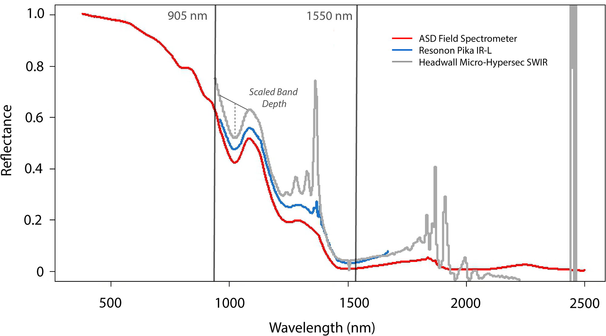
The snow spectral reflectance averaged across ground measurement locations on 18 March. No additional processing was done to remove or reduce noise for direct comparison of reflectance signatures across instruments. Overlaid are lines indicating the wavelengths of lidar sensors (miniVUX1 and VUX-120) and example of scaled band depth used in forward modeling.

Figure 2 Long description
The y-axis label is Reflectance, with tick labels at 0, 0.2, 0.4, 0.6, 0.8, and 1.0. The x-axis label is Wavelength (nm), with tick labels at 500, 1000, 1500, 2000, and 2500. The legend lists ASD Field Spectrometer, Resonon Pika IR L, and Headwall Micro Hyperspec SWIR. Two vertical reference lines are labeled 905 nm and 1550 nm. Text near the curves reads Scaled Band Depth, with a leader line to a trough region and a dashed vertical segment drawn between a higher curve level and a lower point in that region. The ASD Field Spectrometer line starts near the 1.0 tick at the low wavelength end and declines toward the 0 tick by around the 1500 tick, then stays close to the 0 tick through the 2500 tick. The Resonon Pika IR L line follows a similar path through the 1500 tick and ends shortly after the 1500 tick. The Headwall Micro Hyperspec SWIR line includes multiple narrow spikes between the 1000 and 2000 ticks, and two very tall narrow spikes near the 2500 tick.
To evaluate lidar-based snow grain size retrievals as a function of wavelength, two Riegl lidar instruments were also flown as part of the comparison: (1) Riegl miniVUX1 and (2) Riegl VUX-120. The Riegl miniVUX1 weighs 1.5 kg and has a 905 nm laser. The Riegl VUX-120 weighs 2.3 kg and has a 1550 nm laser. The miniVUX1 was flown on a Vulcan Raven Heavy Lift UAS. The VUX-120 was flown on a Harris Aerial Carrier Hx8 UAS. The price point of the miniVUX1 airborne payload used here is ∼$100k, whereas the VUX-120 is ∼$200k.
Flights were consecutively flown, planned with terrain following altitude mode, and 50% swath across track overlap. Each platform recorded high precision IMU and Real-Time or Post-Processed Kinematic (RTK/PPK) GNSS data for geolocation. Ground control points and field spectrometer locations were surveyed using a GNSS rover and were PPK-corrected with the nearby Pilot Peak reference station. On 18 March, flights focused on comparing data collected with similar ground sampling distance (GSD). The first flight started at 1:34 pm MDT and the final flight started at 4:29 pm MDT (see Table 1 for flight order and details). The field spectrometer measurements started at 2:00 pm. On 19 March, flights focused on data collection at different flight altitudes to assess trade-offs between atmospheric spectral noise, spatial resolution and coverage. The first flight was at 12:53 pm MDT and the last flight was at 3:21pm MDT. The field spectrometer measurements started at 12:30 pm MDT.
Overview of sensors, UAS, flight altitude, and flight date and start times.

2.1. Grain size retrievals
For both field and imager reflectance, grain size retrievals followed the same general workflow. The compact imager spectral responses were converted to reflectance using a ‘gray’ in-scene calibration target with known flat spectral reflectance. Because flights were conducted at low altitude (40–120 m above ground level (AGL)), atmospheric path radiance and transmittance effects were minimal; conversion to reflectance using the target (empirical line calibration) implicitly accounts for these short-path atmospheric influences, and no additional radiative transfer based atmospheric correction was applied. Each imager’s manufacturer software was used for radiometric calibration and orthorectification using the same lidar digital elevation model (DEM). Individual flight lines were mosaicked and resampled to 0.5 m resolution. The non-snow pixels were masked using a reflectance threshold (0.3, applied to imagers at 1030 nm and single wavelength lidar).
The scaled band depth (SBD; Clark and Roush, Reference Clark and Roush1984) of the first ice absorption feature, centered at 1030 nm, was computed for each reflectance spectrum (Fig. 2). The SBD continuum normalizes the ice absorption feature and then calculates the depth to the center of the feature, which scales nonlinearly with grain size. The SBD is less sensitive to liquid water content than full band-area metrics (Donahue and others, Reference Donahue, Skiles and Hammonds2022). A lookup table (LUT) of modeled snow reflectance was generated using the Asymptotic Analytical Radiative Transfer model (ART; Kokhanovsky and Zege, Reference Kokhanovsky and Zege2004) for grain sizes from 30 to 2000 µm under the flight specific solar zenith angle. Measured SBDs were matched to modeled values to retrieve effective grain radius for each point or pixel.
For lidar data, points were processed to produce a consistent GSD, and then conversion to reflectance and grain size retrievals followed Ackroyd and others (Reference Ackroyd, Donahue, Menounos and Skiles2024). Briefly, lidar intensity values were corrected for range and incidence angle using the lidar altimetry, then converted to reflectance using calibration factors derived from co-located field reflectance measurements (−0.15 for miniVUX1; −0.32/−0.34 for VUX-120 on 18 March and 19 March, respectively). The active laser source and short atmospheric path length minimize atmospheric attenuation, and no additional atmospheric correction was required. Corresponding single-band ART LUTs were generated at 905 nm and 1550 nm, and grain size was retrieved by matching measured to modeled reflectance per point. The incidence angle correction accounts for local surface slope effects, enabling comparison with ART LUTs generated under planar surface geometry assumptions. The resulting point cloud grain size retrievals were gridded for comparison with imagers.
To describe the central tendency of grain size distribution, the median and standard deviation (σ) were summarized for all flights. To assess against field spectroscopy, grain sizes from UAS datasets were extracted at pixels corresponding to measurement locations, also summarized with median and standard deviation. Accuracy was assessed using the bias, median absolute error (MAE) and average percent error. The number of comparison points (n) is reported as not all field measurement points had a corresponding UAS retrieved value.
3. Results
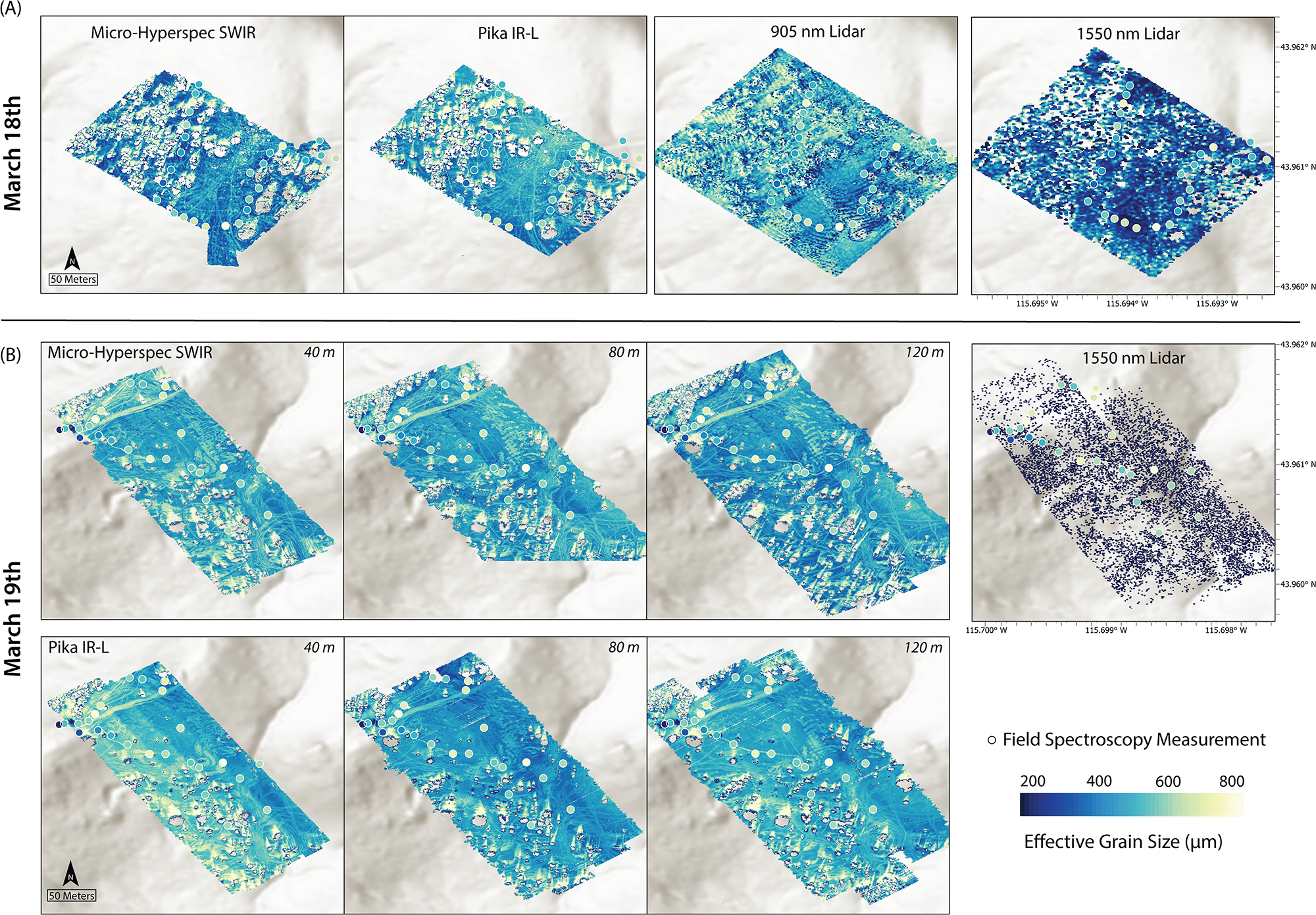
The grain sizes from field spectroscopy were relatively large, consistent with melting snow conditions (Table 2). The grain size retrieval ranged from 298 to 670 µm (median 490 µm, σ = 84 µm) on 18 March and from 238 to 744 µm (median 553 µm, σ = 108 µm) on 19 March. Spectral reflectance from the UAS imagers exhibited higher spectral noise relative to the field reflectance, particularly for the Micro-Hyperspec SWIR; however, both sensors had low noise across the 1030 nm absorption feature used for grain size retrievals (Fig. 2). Grain size maps from the compact imagers and 905 nm lidar captured the expected spatial variability: greater heterogeneity around trees, larger grains in compacted snowmobile and ski tracks, and more uniform, smaller grains in open areas (Fig. 3). Distributions from the compact imagers and the 905 nm miniVUX1 were broader than, but generally consistent with, field spectroscopy (Fig. 4), whereas retrievals from the 1550 nm lidar were strongly biased toward unrealistically low values.
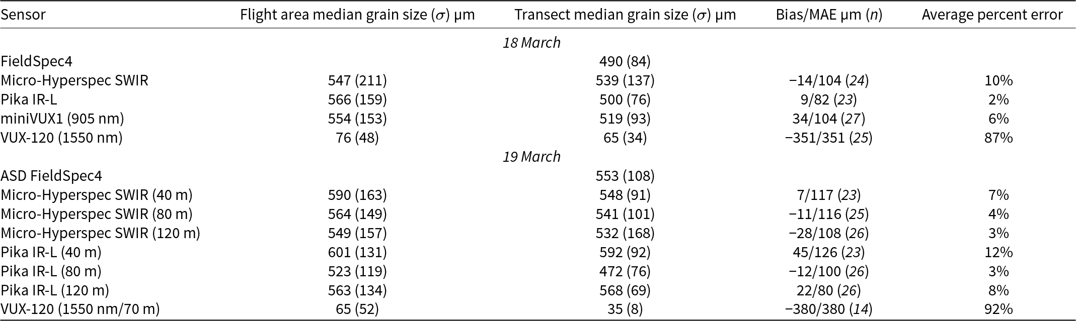
Summary of median grain size and standard deviation retrieved from the field spectrometer, compact imaging spectrometers and lidar instruments as well as error metrics, relative to the reference field spectroscopy measurements, for imaging spectroscopy and lidar grain size retrievals.

Table 2 Long description
Columns: Sensor; Flight area median grain size (sigma) micrometer; Transect median grain size (sigma) micrometer; Bias slash MAE micrometer left parenthesis n right parenthesis; Average percent error. Row 1: 18 March; blank; blank; blank; blank. Row 2: FieldSpec4; blank; 490 (84); blank; blank. Row 3: Micro Hyperspec SWIR; 547 (211); 539 (137); minus 14 slash 104 (24); 10 percent. Row 4: Pika IR L; 566 (159); 500 (76); 9 slash 82 (23); 2 percent. Row 5: miniVUX1 (905 nm); 554 (153); 519 (93); 34 slash 104 (27); 6 percent. Row 6: VUX 120 (1550 nm); 76 (48); 65 (34); minus 351 slash 351 (25); 87 percent. Row 7: 19 March; blank; blank; blank; blank. Row 8: ASD FieldSpec4; blank; 553 (108); blank; blank. Row 9: Micro Hyperspec SWIR (40 m); 590 (163); 548 (91); 7 slash 117 (23); 7 percent. Row 10: Micro Hyperspec SWIR (80 m); 564 (149); 541 (101); minus 11 slash 116 (25); 4 percent. Row 11: Micro Hyperspec SWIR (120 m); 549 (157); 532 (168); minus 28 slash 108 (26); 3 percent. Row 12: Pika IR L (40 m); 601 (131); 592 (92); 45 slash 126 (23); 12 percent. Row 13: Pika IR L (80 m); 523 (119); 472 (76); minus 12 slash 100 (26); 3 percent. Row 14: Pika IR L (120 m); 563 (134); 568 (69); 22 slash 80 (26); 8 percent. Row 15: VUX 120 (1550 nm slash 70 m); 65 (52); 35 (8); minus 380 slash 380 (14); 92 percent.
Snow grain size retrieval maps for compact imagers and lidar instruments on 18 March (top) and 19 March (bottom) at a common resolution of 0.5 m. Field spectroscopy grain size retrievals are mapped for reference, with the value at each point following the same color scale as the maps.

Figure 3 Long description
A) Four thematic maps titled, Micro Hyperspec SWIR, Pika IR L, 905 nm Lidar, and 1550 nm Lidar. Each map contains a rotated rectangular survey footprint filled with a continuous value surface and overlaid circular markers. A north arrow and a scale bar labeled 50 Meters appear at the lower left of the first map. The fourth map has axis ticks with latitude labels 43.960 degrees N, 43.961 degrees N, and 43.962 degrees N on the right edge, and longitude labels 115.695 degrees W, 115.694 degrees W, and 115.693 degrees W along the bottom edge. B) Seven thematic maps arranged as three maps titled, Micro Hyperspec SWIR, with corner labels 40 m, 80 m, and 120 m, plus one map titled, 1550 nm Lidar, and three maps titled, Pika IR L, with corner labels 40 m, 80 m, and 120 m. The survey footprint is a rotated rectangle in each map with circular markers overlaid. A north arrow and a scale bar labeled 50 Meters appear at the lower left of the first map in this group. The 1550 nm Lidar map has axis ticks with latitude labels 43.960 degrees N, 43.961 degrees N, and 43.962 degrees N on the right edge, and longitude labels 115.700 degrees W, 115.699 degrees W, and 115.698 degrees W along the bottom edge. Legend and symbols: A hollow circle is labeled, Field Spectroscopy Measurement. A horizontal scale is labeled 200, 400, 600, and 800, with the label, Effective Grain Size (um).
Grain size distributions visualized as violin plots for flights and field measurements on 18 March (above) and 19 March (below). The violin plots extend from the 2nd to 98th percentile, and the interquartile range and median are overlaid in each plot.

Figure 4 Long description
A) March 18. Violin plots. The vertical axis label is, Grain Size (micrometer), with tick labels 100, 200, 300, 400, 500, 600, 700, 800. The horizontal axis categories are, Micro-Hyperspec SWIR, Pika IR-L, 905 nanometer Lidar, 1550 nanometer Lidar, Field Spectrometer. A key at the top right labels, Interquartile Range, and, Median. Each violin includes a vertical interquartile range line and a circular median marker. Micro-Hyperspec SWIR median is just below 500, and the interquartile range spans from just above 400 to just below 600. Pika IR-L median is just above 500, and the interquartile range spans from just below 500 to just above 600. 905 nanometer Lidar median is between 500 and 600, and the interquartile range spans from just below 500 to just above 600. 1550 nanometer Lidar median is just above 100, and the interquartile range spans from just above 100 to around 150. Field Spectrometer median is just below 500, and the interquartile range spans from the mid 400s to just above 500. B) March 19. Violin plots. The vertical axis label is, Grain Size (micrometer), with tick labels 100, 200, 300, 400, 500, 600, 700, 800. The horizontal axis shows grouped categories separated by vertical divider lines. Group label, Pika IR-L, with three violins labeled 40 m, 80 m, 120 m. Group label, Micro-Hyperspec SWIR, with three violins labeled 40 m, 80 m, 120 m. Then a single violin labeled, 1550 nanometer Lidar. Then a single violin labeled, Field Spectrometer. Each violin includes a vertical interquartile range line and a circular median marker. Pika IR-L 40 m median is between 500 and 600, and the interquartile range spans from just above 500 to the mid 600s. Pika IR-L 80 m median is around 500, and the interquartile range spans from the high 400s to the mid 500s. Pika IR-L 120 m median is just above 500, and the interquartile range spans from about 500 to just below 600. Micro-Hyperspec SWIR 40 m median is between 500 and 600, and the interquartile range spans from about 500 to just above 600. Micro-Hyperspec SWIR 80 m median is just above 500, and the interquartile range spans from just below 500 to about 600. Micro-Hyperspec SWIR 120 m median is just above 500, and the interquartile range spans from just below 500 to just below 600. 1550 nanometer Lidar median is just above 100, and the interquartile range spans from just above 100 to around 150. Field Spectrometer median is between 500 and 600, and the interquartile range spans from about 500 to about 600.
On 18 March, the median grain size at field measurement points from the Micro-Hyperspec SWIR flight was 539 µm (σ = 104 µm), slightly higher and more variable than the Pika IR-L (500 µm, σ = 76 µm). The bias and error were higher for the Micro-Hyperspec SWIR (−14 µm bias, MAE = 104 µm) than the Pika IR-L bias (9 µm bias, MAE = 82 µm), which had the lowest percent error across all flights (2%) (Table 2). The 905 nm miniVUX1 retrievals were comparable to the imagers, with median grain size of 519 µm (σ = 93 µm) and moderate positive bias (34 µm). The poorest performance was the 1550 nm VUX-120, with the low median grain size (76 µm, σ = 48 µm) resulting in high bias and error.
On 19 March, the Micro-Hyperspec SWIR showed a potential weak dependence on flight altitude; variability and bias magnitude increased with altitude whereas MAE and percent error decreased (Table 2). The Pika IR-L displayed no clear altitude trend; the highest error was at 40 m, which had the most obvious line-to-line differences, potentially due to changing illumination or processing (Fig. 3). Excluding the 40 m flight, both imagers yielded similar accuracy (≤10% error), with the Pika IR-L performing comparably to the higher resolution Micro-Hyperspec SWIR. The 1550 nm VUX-120, which was not a part of the altitude test but was flown at the same flight altitude as the day prior, was again biased toward small grain sizes with large negative bias and error.
Comparing across the full extent of the maps, the Micro-Hyperspec SWIR, Pika IR-L and 905 nm miniVUX1 maps showed coherent structure in grain size across terrain, with similar contrasts between open and shaded or compacted areas. The 905 nm lidar produced grain size distributions and spatial patterns like those from the imagers, although the shape of the distribution was normal, whereas other distributions were right-skewed, toward smaller grains (Fig. 4). As expected under reduced local illumination (e.g. tree-cast shadows), the imagers exhibited increased bias, whereas the actively illuminated 905 nm lidar was comparatively less sensitive to shadowing effects. This highlights the relative robustness of lidar-based retrievals under variable or suboptimal illumination conditions. In contrast, the 1550 nm VUX-120 lidar yielded physically implausible results due to weak return intensities and lower point densities in snow-covered areas.
When flight altitude and instrument configuration were controlled (18 March) to yield comparable GSDs, the two imagers and the 905 nm lidar produced similar grain-size distributions. On 19 March, when GSDs diverged, the Micro-Hyperspec SWIR and Pika IR-L still maintained relatively good agreement across flight altitudes and with reference data, indicating limited sensitivity to spatial resolution over the tested range. The 1550 nm lidar was flown at the same altitude on both days, with sparse and strongly biased retrievals on both days, confirming that snow absorption at this wavelength precludes meaningful grain size mapping. The sparser returns on 19 March likely resulted from increased surface meltwater. The impact of liquid water on retrievals is covered in more detail in the discussion.
Together, these results demonstrate that compact UAS imaging spectrometers and 905 nm lidar can retrieve snow grain size within ∼10% error relative to field spectroscopy, even under melting-snow conditions. The comparable accuracy of Pika IR-L and the 905 nm miniVUX1 lidar suggests that both instruments provide viable, scalable options for operational UAS snow surveys at lower price points. Conversely, SWIR lidar at 1550 nm is not suitable for snow grain size retrieval due to high absorption in this region.
4. Discussion
The consistency in median values and distribution shapes across sensors supports the robustness of the retrievals (Fig. 4). However, the MAE (∼100 µm) for the imagers and 905 nm lidar indicated relatively poor comparison across a subset of ground reference points. The error is higher than what is typically reported for reflectance based grain size uncertainty, which is 50 µm for grain sizes between 50 and 900 µm (e.g. Nolin and Dozier, Reference Nolin and Dozier2000). The error could reflect differences in spatial resolution, imperfect georeferencing and temporal offset between collections and measurement error. With sunny conditions, warm air temperatures and observable melt, it is reasonable that a difference of tens of minutes could contribute to actual differences in grain size. However, field spectroscopy was started prior to the imager and 905 nm lidar flights but field grain size retrievals were not consistently smaller.
Collecting high quality field spectroscopy measurements in snow covered environments can be challenging and there were indications of measurement error (SI Fig. 1). Physically, values in the visible wavelengths should not be higher than one, although they can occur with directional reflectance measurements over freshly fallen (highly reflective) snow because the white reference is lambertian, it scatters equally in all directions, and snow is forward scattering. However, with older melting snow this can indicate that the foreoptic was not oriented nadir to the surface. There was also high variability on 19 March across the visible wavelengths in reflectance magnitude; patterns that can happen when the white reference does not encompass the full field of view. Additionally, the foreoptic footprint (∼25 cm) likely was not always measuring homogeneous snow given surface variability; small-scale surface roughness (e.g. microtopography, disturbed compacted snow) may have contributed to variability in measured reflectance.
However, the SBD grain size retrieval method reduces sensitivity to illumination and measurement error because it does not use absolute reflectance magnitude. The continuum normalized ice absorption feature exhibited less variability relative to the full spectral reflectance curves (SI Fig. 1). However, the positive bias in tree shadows and flight line artifacts in imager grain size maps indicates persistent sensitivity to illumination conditions (Fig. 3). It is interesting to note that the center of the ice absorption feature for dry snow is 1030 nm, whereas for reflectance measured in this study it was 1020 nm (SI Fig. 1), which is not error but rather indicates the presence of liquid water. Water absorption is offset to a shorter wavelength from ice such that the left shoulder of the ice absorption widens when water is present in snow (see Fig. 12 in Donahue and others, Reference Donahue, Skiles and Hammonds2022).
Typically, surface grain size mapping is used as a proxy for snow energy balance, snow age and snow albedo. For context, new snow grain sizes are typically on the order of 100 µm (Skiles and others, Reference Skiles, Donahue, Hunsaker and Jacobs2023), older melting season snow grain sizes can range between 500 and 800 µm (Seidel and others, Reference Seidel, Rittger, Skiles, Molotch and Painter2016; Skiles and Painter, Reference Skiles and Painter2017), and grain sizes for exposed glacier ice can extend past 2000 µm (Donahue and others, Reference Donahue2023). However, the relationship between grain size and albedo is nonlinear, and albedo is less sensitive to change at larger grain sizes (SI Fig. 2). Therefore, it can be useful to translate grain size error to error in albedo and net solar radiation.
Using the grain size and solar zenith angle, the ‘clean snow’ broadband albedo was modeled by spectrally weighting and integrating modeled albedo with downwelling irradiance (e.g. Skiles and others, Reference Skiles, Donahue, Hunsaker and Jacobs2023; Ackroyd and others, Reference Ackroyd, Donahue, Menounos and Skiles2024). Spectral irradiance was not directly measured and was therefore modeled under clear-sky conditions using the Santa Barbara DISORT Atmospheric Radiative Transfer model (SBDART; Ricchiazzi and others, Reference Ricchiazzi, Yang, Gautier and Sowle1998) for solar noon on 18 March. The integrated downwelling shortwave irradiance was 700 W m−2, a reasonable clear-sky mid-March value for this latitude. Although modeling solar irradiance introduces uncertainty in the absolute net (absorbed) solar radiation, it does not affect the relative comparison among sensors, as proportional scaling of irradiance would apply to all retrievals.
On 18 March, the range of grain sizes retrieved from field spectroscopy was 298–670 µm with a corresponding range in albedo of 0.74–0.69. Reporting at two significant digits, the median albedo (0.71) was the same for the field spectrometer, Micro-Hyperspec SWIR, Pika IR-L and 905 nm minVUX1 lidar, and was 0.78 for the 1550 nm VUX120 lidar, at field measurement locations. The net solar radiation for the field spectroscopy albedo was 203 W m−2. For the Micro-Hyperspec SWIR, Pika IR-L and 905 nm lidar, respectively, it would have been 201 W m−2 (0.7% error), 204 W m−2 (0.5% error) and 205 W m−2 (1.3% error). Although the errors in grain size were high, because grain sizes were relatively large, the implications for modeling albedo and net solar radiation were minor. For the 1550 nm lidar the net solar radiation error would have been 152 W m−2 (25% error), which is prohibitively high.
When comparing instruments, it is worthwhile to consider technical specifications, accuracy, dataset volume and cost. Despite differences in instrument specifications both imagers accurately resolved the 1030 nm absorption feature used for grain size retrieval and performed similarly. The errors and bias were not consistent across flights, with the Pika IR-L having lower error on 18 March and the Micro-Hyperspec SWIR having generally lower error on 19 March. The propagation of error to net solar radiation (<1%) reinforces similarity and puts grain size errors in context. A notable difference is that the Micro-Hyperspec SWIR produces data volumes nearly 20 times larger than the Pika IR-L, due to broader spectral range and higher spatial resolution, increasing storage needs and processing time. Across different factors, the Pika IR-L is an appealing and suitable choice for grain size mapping.
However, if snow grain size is not the only intended retrieval, the extended wavelength range of the Micro-Hyperspec SWIR could be advantageous. Additionally, the imagers compared here would need to be paired with a visible sensor to directly map broadband albedo in environments influenced by spatially and temporally varying light-absorbing particles (LAPs; Skiles and others, Reference Skiles, Flanner, Cook, Dumont and Painter2018), which primarily reduce albedo in the visible wavelengths. The broadband albedo modeling presented here assumed clean snow, neglecting darkening by LAPs. The Headwall coaligned system is designed for spectral reflectance measurements across the solar spectrum, whereas Resonon makes a visible-NIR compact imager but does not have an integrated coaligned system.
The 905 nm miniVUX1 lidar performed comparably to the compact imagers for grain size with similar propagation of error to albedo (∼1%). The close agreement highlights the potential of single wavelength lidar intensity as a practical alternative where passive acquisitions are not collected or are limited by suboptimal illumination conditions due to shadows, low sun angles or variable cloud cover. Although more expensive than the Resonon Pika IR-L, the 905 nm miniVUX1 can map both topography and grain size, which may be appealing to end users who are interested in complementing altimetry, and volume characterization, with an indicator of snow age and energy balance.
By contrast, the 1550 nm VUX-120 lidar exhibited unrealistically small grain sizes, resulting in a strong negative bias and high error. These errors result from strong absorption by ice past 1500 nm (Fig. 2), which reduces return intensity and signal-to-noise ratio. It was challenging to interpret the potential impact of liquid water on the lidar retrievals. Across the NIR and SWIR, both ice and water are increasingly absorptive; at 905 nm there is moderate absorption, with water absorbing more than ice and at 1550 nm there is strong absorption, with ice being more absorptive than water (see Fig. 1 in Donahue and others, Reference Donahue, Skiles and Hammonds2022). The 905 nm lidar comparison to field and imaging spectroscopy indicated no obvious impact from melt water, whereas the 1550 nm lidar was potentially impacted by water on 19 March; the flight was later in the day, when there would be more water in the snow. Despite flight parameters being the same between both days, the point cloud had sparser returns and there was lower intensity. This could have implications for quality of topographic mapping using 1550 nm lidar over snow.
The outcome of the 19 March flights indicated altitude effects on retrieval accuracy were minimal within the 40–120 m tested range. For the Micro-Hyperspec SWIR, variability increased and MAE decreased modestly from 40 m to higher altitudes. The Pika IR-L showed no monotonic trend with altitude, with the highest error at 40 m, likely related to line-to-line illumination changes. These results suggest that, within typical UAS operational envelopes, atmospheric path length and spatial resolution have a secondary influence compared with surface heterogeneity and illumination geometry.
5. Conclusion
This study provides the first quantitative comparison of snow grain size retrievals from commercially available UAS-mounted imaging spectrometers and lidars. The intercomparison effort demonstrated that compact imaging spectrometers mounted on UAS can retrieve snow grain size comparable to field spectroscopy. The 905 nm lidar achieved comparable performance to the imaging spectrometers, demonstrating that active, single-wavelength measurements can supplement passive optical systems, decoupled from natural illumination conditions. In contrast, the 1550 nm lidar exhibited severe negative bias (>90% error) due to strong SWIR absorption by ice and water; this wavelength is unsuitable for snow property retrievals, especially when snow is melting.
From a practical standpoint, these findings indicate that compact spectrometers and low-cost 905 nm lidar can provide physically realistic estimates of snow grain size with error ≤10% and net solar radiation error <1% while differing substantially in cost, technical specifications and data volume. The 905 nm lidar can additionally provide surface elevation, both valuable retrievals for studying snow evolution. These results highlight the potential for cost-effective, lightweight UAS sensors to generate quantitative maps of snow properties. The comparable performance of lower-cost instruments expands opportunities for distributed time-series monitoring.
Supplementary material
The supplementary material for this article can be found at https://doi.org/10.1017/jog.2026.10156.
Acknowledgements
We gratefully acknowledge Brent Wilder, Joachim Meyer and Jeremy Johnston for their support in acquiring the ASD measurements. This material is based upon work supported by the Broad Agency Announcement Program and the Cold Regions Research and Engineering Laboratory (ERDC-CRREL) under Contracts W913E521C0006 and W913E523C0004. Distribution A: Approved for public release. Distribution is unlimited.




 Open access

