1. Introduction
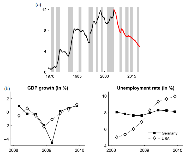
In its recent past, the German economy has experienced a labor market miracle:Footnote 1 The unemployment rate, having trended upwards since the 1970s to record highs of what observers called the “sick man of Europe” (Dustmann et al. Reference Dustmann, Fitzenberger, Schönberg and Spitz-Oener2014), halved within a decade; a decade in which the Great Recession hit and triggered the largest output loss in postwar German history (Figure 1).Footnote 2 The German labor market miracle consists of these two interrelated aspects: a strong and permanent fall in unemployment that set in in 2005, and an exceptionally low increase of unemployment during the Great Recession compared to other crisis-hit countries like the USA.
The German labor market miracle. (a) Unemployment rate and economic downturnsFootnote 3 in Germany (b) GDP growth and unemployment rate in Germany and USA during the Great Recession.

What makes this favorable development particularly interesting, in addition to its unprecedented character and the simultaneous occurrence of a serious economic crisis, is that it was preceded by significant labor market (“Hartz”) reforms. These reforms are an obvious candidate cause and often referred to. However, the literature is by no means unanimous on their effects; not least because the methodological approaches differ, because some studies focus on specific aspects while ignoring others and because the reform measures were not homogeneous, but had different macroeconomic effects (see the literature survey below). Beyond policy, other developments have also been put forward to explain the German labor market miracle, ranging from favorable economic conditions (before and following the crisis) to general wage restraint. This article strives for a comprehensive assessment of all potential factors that may have contributed to the labor market miracle and to identify them within a single consistent macroeconometric framework.
To this end, we estimate vector autoregressions (VARs) on quarterly German data ranging from 1970 to 2018 and identify demand, technology, labor supply, wage bargaining, and matching efficiency shocks through robust sign restrictions as proposed by Foroni et al. (Reference Foroni, Furlanetto and Lepetit2018). These five structural shocks are particularly well-suited to investigate the German labor market miracle: The identification of business cycle (aggregate demand and technology) shocks allows us to carve out the effects of the Great Recession and the preceding and subsequent booms. The identified labor market shocks, on the other hand, capture well the variety of undertaken reforms: the improvement of matching efficiency through the re-organization of the Employment Agency (Hartz III), a fundamental change of the workers’ outside option through the reduction of wage replacement benefits and a movement from out of labor force into labor supply (both through Hartz IV). However, the identified labor market shocks also capture developments other than policy measures that are potentially relevant for the German labor market miracle. These may include a general tendency to wage restraint and changes in labor supply due to demographic shifts.
Our structural VAR approach addresses important drivers of labor market fluctuations. In contrast to the existing literature on the German labor market miracle, it enables us to not only focus on the radical policy reform measures that were implemented in the 2000s, but also to account for several other aspects within a coherent macroeconometric framework. On the other hand, this rather broad perspective does not allow us to differentiate analytically between policy measures and policy-unrelated developments. However, we can say something about the timing of certain shocks. In particular, we find a significant increase in labor supply (and a corresponding increase in unemployment) in the year in which Hartz IV came into effect (2005) while over the entire sample, a contraction in labor supply prevailed. Moreover, wage moderation was absent in the early 2000s, but it was particularly pronounced in 2006.
We find that wage bargaining shocks account for most of the strong decline in unemployment. Wage restraint was exceptionally pronounced right after the implementation of Hartz IV, pointing to a vital role of it in reducing reservation-wage-related unemployment. However, we also find that wage moderation persisted far beyond the introduction of Hartz IV, albeit more muted. Our tentative exploration on this persistence points to the European monetary union (EMU): by running the model over different sample periods, we are able to confirm the theoretical result that EMU has enhanced the positive real effects of country-specific wage moderation due to the absence of a compensating exchange rate mechanism (appreciation). This might have made wage moderation a worthwhile strategy for both employers and workers in Germany to pursue. But the labor market miracle is not monocausal. In our baseline specification, wage moderation reduced the unemployment rate by 3.5 percentage points, improvements of matching efficiency by 1.3 percentage points, and a contraction of labor supply by one percentage point.
Business cycle shocks reduced it by a further 0.7 percentage points, which is noteworthy because it shows that the recovery has outweighed the impact of the Great Recession on unemployment. However, we find that the response of unemployment to business cycle shocks is generally low in Germany. To be precise, business cycle shocks account for less than 20% of unemployment fluctuations, while in the USA they are found to account for up to half of it in the short run (for a similar response of output). This essentially explains the small increase in unemployment during the Great Recession. While the extensive margin of labor barely reacts to business cycles, the intensive margin bears the brunt of adjustment. In an extension of the baseline model, we find that hours worked practically mirror the output fluctuations that are induced by business cycles fluctuations. The strong adjustment of hours worked during the Great Recession, which can be explained by the widespread use of short-time work arrangements in the German economy, helped to keep the rise in unemployment low.
The paper is structured as follows. In the next section, we provide an overview of the literature on the German labor market miracle and discuss how our paper contributes to this literature. In Section 3, we describe the empirical approach and the identifying assumptions. Section 4 gives an overview of the properties of the model, focusing on impulse responses and forecast error variance decompositions. In Section 5, we study the underlying causes of the significant fall in unemployment. Section 6 takes a closer look at the unique period surrounding the Great Recession and the corresponding small increase in unemployment. Finally, Section 7 concludes.
2. Related Literature
Our study contributes to the recent and still growing literature on the causes of the German labor market miracle. Many of these studies focus on the effects of the Hartz reforms that were enacted between 2003 and 2005. Carrillo-Tudela et al. (Reference Carrillo-Tudela, Launov and Robin2021) provide an excellent overview of this strand of the literature. They argue that the differing results regarding the effects of the Hartz reforms are basically due to different assumptions regarding the size of their impulse.
For example, Krebs and Scheffel (Reference Krebs and Scheffel2013) find that the first three reform packages (Hartz I–III) reduced the noncyclical part of unemployment by 1.5 percentage points, while the fourth package (Hartz IV) reduced it by a further 1.4 percentage points. According to Krause and Uhlig (Reference Krause and Uhlig2012), the latter led to a reduction in German unemployment by 2.8 percentage points and also reduced its duration. Hochmuth et al. (Reference Hochmuth, Kohlbrecher, Merkl and Gartner2021) estimate the unemployment dampening effect of Hartz IV at 2.2 percentage points.
Launov and Wälde (Reference Launov and Wälde2016), on the other hand, conclude that it only accounts for 5% of the overall decline in unemployment, while Hartz III, that is, the improvement of the public employment agencies’ effectiveness, explains about 20% of it. The minuscule Hartz IV effect echoes the authors’ earlier results (Launov and Wälde Reference Launov and Wälde2013). Bradley and Kügler (Reference Bradley and Kügler2019) even find that none of the reform measures reduced unemployment substantially, while they acknowledge the dampening effect on the duration of unemployment.
At the other end of the spectrum, Hartung et al. (Reference Hartung, Jung and Kuhn2018) assign almost all of the decline of unemployment since 2005 to the Hartz reforms. They arrive at this conclusion by accounting for separation rates as an important transmission channel of the reforms. This, in turn, is rebutted by Carrillo-Tudela et al. (Reference Carrillo-Tudela, Launov and Robin2021) who argue that accounting for nonparticipation is key to capturing the underlying dynamics properly. Beyond that, Fahr and Sunde (Reference Fahr and Sunde2009) find that Hartz I–III improved the matching process, while Klinger and Rothe (Reference Klinger and Rothe2012) assess that the reforms particularly reduced long-term unemployment.
We do not report another estimate for the presumed effects of the Hartz reforms. Instead of looking at their effects in isolation, we take an encompassing approach by identifying different macroeconomic shocks and discussing the potential role of the labor market reforms as a root cause of these shocks. For example, we find that a significant wage bargaining shock hit the German economy exactly at the time when Hartz IV came into effect. At the same time, Hartz IV cannot be reduced to an exogenous change of workers’ wage bargaining power. It also brought more people to work and, hence, constituted a positive labor supply shock. Similarly, the identified wage bargaining shocks cannot be reduced to the ramifications of Hartz IV, as we also find them in later years. While we think that this “systematic” occurrence of wage restraint is also related to other factors than labor market reforms—in particular, to favorable conditions in a monetary union—our approach allows us to examine it within a single structural (wage bargaining) shock.
Another strand of the literature on the German labor market miracle accounts for the Great Recession. For example, Bauer and King (Reference Bauer and King2018) consider the labor market reforms in conjuncture with the Great Recession, arguing that there might have been offsetting effects. Burda and Hunt (Reference Burda and Hunt2011) focus on the “missing” increase of unemployment during the Great Recession in Germany and find that this was mainly a compensation for firms’ reticence to hire new staff during the preceding expansion, but that wage moderation and the widespread adoption of working time accounts also played a role. Boysen-Hogrefe and Groll (Reference Boysen-Hogrefe and Groll2010) emphasize the role of wage moderation for the small response of unemployment during the Great Recession; they find that the preceding labor market reforms had a certain stake in it.
Gehrke et al. (Reference Gehrke, Lechthaler and Merkl2019) estimate a dynamic stochastic general equilibrium (DSGE) model with a detailed labor market block and show that the labor market reforms were most likely the key drivers of a series of positive labor market performance shocks that hit the German economy prior to the Great Recession and prevented unemployment to increase by more during the recession. Our VAR approach is complementary to their theoretical analysis but also allows for a further decomposition of the underlying labor market innovations that occurred in the years prior to the Great Recession.
3. Empirical Framework
In the following, we describe the empirical model and the identifying assumption of the structural shocks. Let
 \begin{align}\textbf{y}_{\textbf{t}}=\textbf{c}+\sum_{i=1}^{l}\textbf{A}_{\textbf{i}} \textbf{y}_{\textbf{t}\boldsymbol{-}\textbf{i}}+\textbf{u}_\textbf{t},\end{align}
be the reduced-form model, where
 $\textbf{y}_t$
is a vector of endogenous variables,
 $\textbf{c}$
is a vector of constants,
 $\textbf{A}_i$
are reduced-form parameter matrices and
 $\textbf{u}_t\sim\mathcal N(0,\textbf{V})$
is a vector of stochastic error terms. In our baseline specification
 $\textbf{y}_{\textbf{t}}$
includes five variables: log real gross domestic product (GDP), the year-on-year difference of log consumer prices (inflation), log real wages per capita, the registered unemployment rate, and log vacancies.Footnote 4 All data are at a quarterly frequency, seasonally adjusted (except for prices) and cover the period 1970q1 to 2018q1, which provides information on 193 observations (Figure 15). The model is estimated with variables in levels and Bayesian techniques, employing a diffuse Normal–Wishart prior on
 $\textbf{A}=\left[\textbf{c},\textbf{A}_1,\ldots,\textbf{A}_l\right]$
and
 $\textbf{V}$
. The baseline specification includes five lags.
To recover orthogonal innovations
 $\textbf{w}_t=\textbf{Bu}_t$
(with
 $\textbf{V}_{\textbf{w}}$
diagonal), we resort to a method that has become popular in the empirical macro literature (Rubio-Ramírez et al. Reference Rubio-Ramírez, Waggoner and Zha2010). The structural impact multiplier matrices
 $\textbf{B}^{\boldsymbol{-1}}$
are chosen as the product of the Cholesky factor of
 $\textbf{V}$
and orthogonal matrices
 $\textbf{Q}$
obtained via a QR decomposition of matrices sampled from a standard Normal distribution.Footnote 5 From the infinite set of
 $\textbf{Q}$
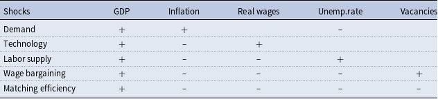
’s, we chose those that lead to appropriate structural models, that is, draws with structural shocks satisfying the impact sign restrictions given in Table 1.
These sign restrictions have been proposed by Foroni et al. (Reference Foroni, Furlanetto and Lepetit2018) who study the contribution of business cycle and labor market shocks in the USA. The restrictions are derived from a New Keynesian DSGE model with search and matching frictions. The baseline model contains five orthogonal shocks: aggregate demand, technology, labor supply, wage bargaining, and matching efficiency shocks. The shocks are normalized such that they induce a positive on-impact GDP response. Sampling stops when one thousand appropriate draws are collected. The set of appropriate draws accounts for estimation uncertainty (by sampling
 $\textbf{A}$
and
 $\textbf{V}$
) and model uncertainty (by sampling
 $\textbf{Q}$
for a given pair of
 $\textbf{A}$
and
 $\textbf{V}$
).
Impact sign restrictions.

A demand shock moves output and prices in the same direction, and output and unemployment in opposite directions. These dynamics are consistent with a variety of disturbances, like, for example, monetary policy, government spending, marginal efficiency of investment, discount factor, and most financial shocks. A productivity (technology) shock, on the other hand, moves output and prices in opposite directions and elicits a positive comovement of output and real wages. The effect on unemployment is unrestricted.
The identified demand and technology shocks represent traditional drivers of the business cycle in standard New Keynesian models. These innovations should be interpreted as shocks which induce fluctuations in real and labor market variables but do not originate from changes in the labor market, in contrast to the remaining three shocks.
An exogenous variation of labor supply, either at the extensive or at the intensive margin, affects the number of job seekers and the ability of firms to fill vacancies. This, in turn, affects hiring costs, wages, and prices. The labor supply shock captures innovations in the labor force due to, for example, demographic changes and migration flows. Moreover, because the Hartz reforms also increased the pool of unemployed officially registered, the labor supply shock might additionally cover parts of the labor market reforms.
A wage bargaining shock constitutes an exogenous variation in real wages originating from the wage bargaining process of workers (trade unions) and employers (firms). Similar to labor supply shocks, this affects firms’ marginal costs and, hence, prices and output. Wage bargaining shocks represent deviations from an average wage setting relation but also exogenous variations in unemployment benefits, which constitute the workers’ outside option in the wage bargaining process.
A matching efficiency shock is associated with similar dynamics but it moves unemployment and vacancies in the same direction. The matching efficiency shock captures variations in the ability of labor market institutions to match workers searching for a job and available vacancies. Improvements in matching efficiency represent better matching technologies in the private job market and public employment agencies.
The restriction of a positive comovement of unemployment and vacancies following a matching efficiency shock deserves some further discussion. As shown in Foroni et al. (Reference Foroni, Furlanetto and Lepetit2018) and Furlanetto and Groshenny (Reference Furlanetto and Groshenny2016), the response of vacancies hinges on the degree of price stickiness. With flexible prices, firms decrease them substantially in response to a positive matching efficiency shock and, as a consequence, aggregate demand rises sharply, prompting firms to hire more staff and, hence, post more vacancies. This, in turn, could outweigh the vacancy reduction originally brought about by the improvement of matching, so that the direction of the impact response of vacancies might be undetermined. This ambiguity is ruled out when prices are sufficiently rigid, so that prices and output react more muted and the response of vacancies to a positive matching efficiency shock is clearly negative.
The latter most probably pertains to the German case, as price rigidity in Germany is high (Gehrke et al. Reference Gehrke, Lechthaler and Merkl2019); so our baseline sign restrictions appear to stand on solid ground. However, given that in the reference model of Foroni et al. (Reference Foroni, Furlanetto and Lepetit2018) vacancies respond unambiguously negative in the second period after impact—independently of the degree of price stickiness—we verify that our main results hold when imposing the sign restrictions on vacancies in the second quarter in a robustness check. We also estimate a four-variable VAR without vacancies, where wage bargaining and matching efficiency shocks are identified jointly as a single “labor demand shock”.
4. Properties of the Model
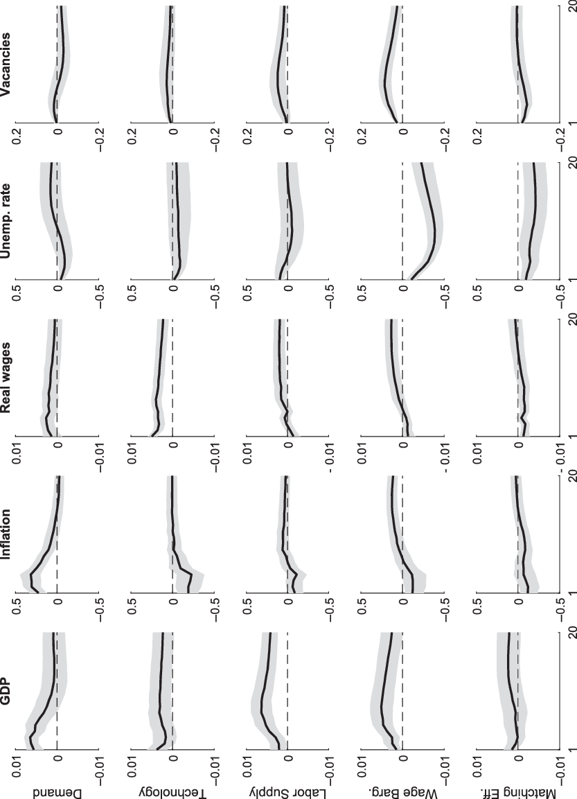
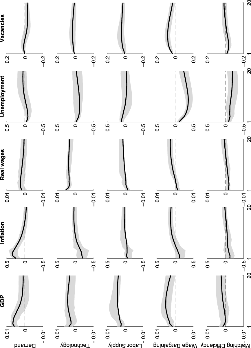
Before quantifying the importance of the different economic shocks for the German labor market miracle, we first gauge the properties of the baseline model by analyzing impulse responses and forecast error variances. Figure 2 shows median impulse responses (solid lines) together with 68% pointwise credible sets (shaded areas) from impact to 5 years after the respective shock. Overall, we obtain impulse responses that are very much in line with economic theory.
Impulse responses. Note: medians and corresponding 68% credible sets.

The response of output, inflation, and unemployment to a demand shock is transitory and lasts for about 1–3 years. GDP and inflation increase significantly with peak responses after around a year. Wages and vacancies, whose impact responses are not restricted, increase in the short run; in the medium run the effects fade out.Footnote 6
The technology shock differs from the demand shock through its divergent response of output and inflation. It elicits more permanent effects on several variables. Output and wages increase significantly and persistently. In contrast, inflation declines significantly with a peak response in the first year after impact. The impact response of unemployment, which is free of identifying restrictions, is small but negative and most draws indicate a persistent decline. Vacancies increase slightly and the increase lasts longer than in demand-fueled booms.
With respect to labor supply shocks, their output effect is initially modest. It strengthens after some time such that in the medium run a clear positive effect prevails. The imposed price dampening effect is short-lived. Also, the impact increase of unemployment abates quickly and the dampening effect on wages reverses at the end of the forecast horizon. The response of vacancies, which is unrestricted, is small on impact and becomes positive at later horizons. This set of impulse responses is well in line with the findings by Foroni et al. (Reference Foroni, Furlanetto and Lepetit2018) for US data and points to the following macroeconomic nexus: an exogenous increase of labor supply and the corresponding reduction of the price of labor incentivize labor demand and, hence, the creation of new vacancies. This demand side repercussion acts as an accelerator of growth and, as a result, counteracts the initial wage and price decline. The labor demand effects following the labor supply shock outweigh the reduction of prices and wages and bring unemployment down again.
Wage bargaining shocks bear similarities to labor supply shocks in several dimensions: with respect to the qualitative response of output (initially modest, then strengthening), vacancies (positive and persistent), inflation, and wages (medium-run compensation of initial decline). The compensating effect on prices seems to be more pronounced for wage bargaining shocks than for labor supply shocks. Correspondingly, the long-term effect of output is more muted. These nuanced differences between the two shocks might follow from the fact that in the case of an exogenous increase of labor supply firms draw from a larger pool of workers (or a larger supply of working hours) when growth accelerates such that inflation pressures are deferred. In case of a wage bargaining shock, on the other hand, unemployment is reduced significantly even in the medium run, while it only settles at its pre-shock level when labor supply expands exogenously.
Unemployment also decreases in a persistent manner in response to an improvement of the matching technology. The response is steadier and less cyclical compared to a wage bargaining shock. In contrast, the impact decrease of vacancies is not permanent. Again, this evidence is well in line with Foroni et al. (Reference Foroni, Furlanetto and Lepetit2018). Another feature of a matching efficiency shock is that the rather blurred short run response of output turns unambiguously positive in the medium run. The dampening price and wage effects fade out over time.
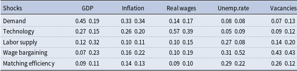
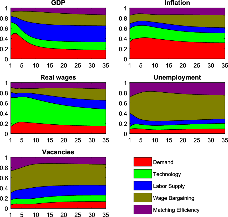
To investigate the quantitative importance of the various structural shocks in driving the endogenous variables, Figure 3 and Table 2 present the average forecast error variance decomposition of our baseline model. Regarding the unemployment rate, there are substantial differences between Germany and the USA. In particular, in Germany, the most dominant driver of the unemployment forecast error variance over all horizons are wage bargaining shocks. A similar pattern can be observed for vacancies with wage bargaining shocks explaining a slightly smaller share. Contrary, as shown by Foroni et al. (Reference Foroni, Furlanetto and Lepetit2018), in the USA the dominant driver of unemployment are matching efficiency shocks. Furthermore, business cycle (i.e. demand and technology) shocks account for much more of the short-run variation in the unemployment forecast error than in Germany (a crucial element for understanding the evolution of unemployment rates during the Great Recession, as we will discuss below). For wages and inflation, there is also a single dominant driver. Inflation is primarily driven by demand shocks, wages by technology shocks. The dominant short-run driver of German GDP are demand shocks accounting for almost half of the contribution in the first quarters after the shock materializes. In the medium run, sources of unexpected output fluctuations are more diverse; this result is again well in line with the findings of Foroni et al. (Reference Foroni, Furlanetto and Lepetit2018) for the USA.
Forecast error variance decomposition for
 $t=1$
and
 $t=20$

Forecast error variance decomposition.

All these findings are robust to several modifications of the baseline model: decreasing the lag length to
 $l=3$
, increasing it to
 $l=7$
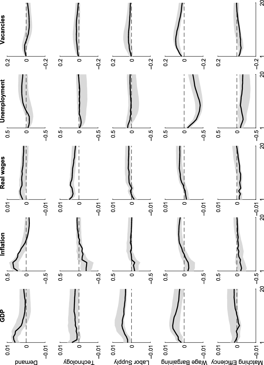
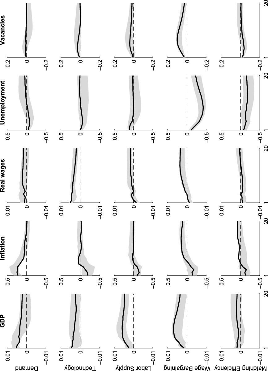
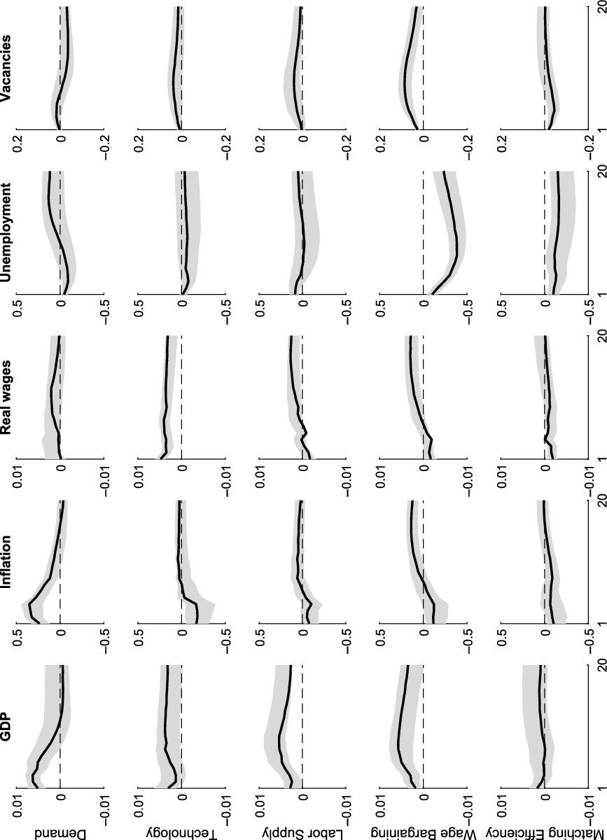
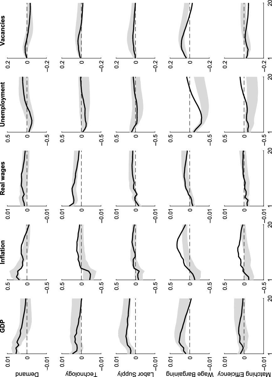
, replacing the consumer price index by the GDP deflator, and replacing per capita wages by wages per hours worked. All median impulse responses of the modified specifications lie within the corresponding 68% credible sets of the baseline specification, as Figures A2, A3, A4, and A5 in the Appendix show.
5. The Labor Market Miracle, Part I
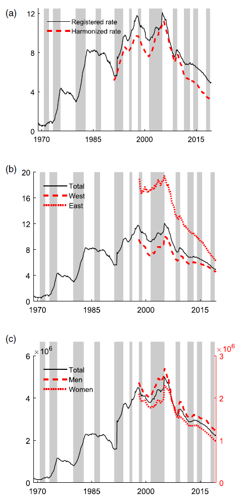
The first aspect of the German labor market miracle is about the steady decline of unemployment that set in 2005 and persisted over more than a decade. Germany has never experienced such a large and persistent drop in the unemployment rate in its postwar history. The unemployment rate more than halved, declining from a peak of 12% in 2005 to below 5% in 2018; a development that was not governed by regional nor gender effects and that is robust to the measurement of unemployment (cf. Figure A1 in the Appendix). In the following, we use the structural VAR model to investigate the quantitative importance of the different economic shocks in explaining the steady decline of unemployment.
5.1. The Decline of Unemployment as a Multifaceted Phenomenon
Our approach enables us to conduct a historical decomposition of the unemployment rate and, hence, to analyze which factors contributed to its decline. A favorable statistical prerequisite for this endeavor is that unemployment was almost zero at the start of the sample period, so that the problem of initial values is mitigated and we have
 \begin{align}ur_t\approx c+\sum_{i=0}^{t-1}\phi_{k,i}w_{k,t-i},\end{align}
where
 $ur_t$
is the unemployment rate at time t, c is a constant,
 $\phi_{k,i}$
is the response of the unemployment rate to shock k in period i, and
 $w_k$
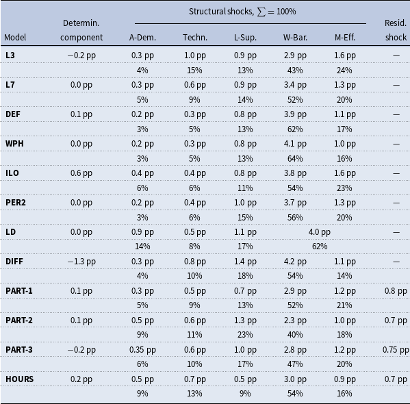
are structural innovations. The main results of the historical decomposition are summarized in Table 3. It presents the average contributions of each structural shock to the cumulative decline of the unemployment rate between 2005 and 2018. The individual contributions add up to 6.5 percentage points, the realized total decline of the unemployment rate over this period.
Decomposition of the unemployment rate 2005–2018 cumulative decline, baseline specification.

Note: A-Dem.: aggregate demand shock, Techn.: technology shock, L-Sup.: labor supply shock, W-Bar.: wage bargaining shock, M-Eff.: matching efficiency shock.
Several interesting results emerge from this exposition: First, the decline of the unemployment rate is not monocausal. Second, each of the identified structural shocks contributes to it to some extent, that is, there are no negative contributions. Obviously, the negative impact of business cycle (i.e. demand and technology) shocks during the Great Recession was more than compensated over the whole period. Labor supply and matching efficiency shock contributed more significantly to the decline in unemployment (1 and 1.3 percentage points, respectively), meaning that labor supply contracted and matching efficiency improved. Third, the largest contribution comes from wage bargaining shocks, accounting for more than half of the unemployment decline in the baseline specification (3.5 percentage points). All three labor market shocks together to explain the fall in unemployment between 2005 and 2018 almost entirely while aggregate demand and technology shocks contribute only to a marginal extent.
Decomposition of the unemployment rate 2005–2018 cumulative decline, further specifications.

L3: lag length
 $l=3$
, L7: lag length
 $l=7$
, DEF: CPI replaced by GDP deflator, WPH: per-capita wages replaced by wages per hour, ILO: registered unemployment rate replaced by harmonized unemployment rate, PER2: sign restrictions on vacancies imposed in the second period, LD: VAR excluding vacancies, with W-Bar. and M-Eff. combined to a joint “labor demand shock”, DIFF: data in first differences, PART: VARs including the participation rate as 6th variable, -1: all available sign restrictions on unemployment imposed, -2: no sign restrictions on unemployment imposed, -3: all available sign restrictions on unemployment imposed except for L-Sup., HOURS: VAR including per-capita hours worked as 6th variable.
In Table 4, we present the results of the historical decomposition for the robustness exercises already mentioned—variation of the lag length (“L3”, “L7”), different measures for prices and wages (“DEF”, “WPH”)—as well as for several further modifications of the model to validate these key results as comprehensively as possible. Specifically, we replace the registered unemployment rate with the harmonized rate (“ILO”), impose sign restrictions on vacancies in the second period instead on impact (“PER2”) to address the ambiguity of the sign restriction for a matching efficiency shock for various degrees of price stickiness, as mentioned earlier. We estimate a 4-variable VAR excluding vacancies and combining matching efficiency and wage bargaining shocks to a single joint “labor demand shock” (“LD”), we estimate the baseline specification with data in first differences (“DIFF”), and we estimate several 6-variable VARs, with the participation rate (“PART’) or hours worked (“HOURS”) as an additional variable.
Since the participation rate and the unemployment rate respond with the same sign to labor market shocks (see Foroni et al. Reference Foroni, Furlanetto and Lepetit2018), we can leave several or all signs on the unemployment rate unrestricted, as the shocks are then identified through the sign restrictions set on the participation rate. We estimate a model with the unemployment rate fully unrestricted (“PART-2”) and a model with only the restriction on labor supply shocks lifted (“PART-3”), as this one is contested in the literature (with, e.g. d’Albis et al. (Reference d’Albis, Boubtane and Coulibaly2021) and Furlanetto and Robstad (Reference Furlanetto and Robstad2019) finding evidence against it, while, for example, Schiman (Reference Schiman2021) argues in favor of it). We compare the results of these specifications with the ones where all sign restrictions on the unemployment rate remain imposed (“PART-1”). While this approach follows the evidence of Canova and Paustian (Reference Canova and Paustian2011), that is, the more restrictions the better for identification provided that the restrictions are theoretically solid, lifting restrictions on unemployment may reveal whether and to what extent the results are driven by them. We find that without the restrictions on unemployment, the role of wage bargaining shocks declines somewhat (mostly at the expense of labor supply shocks) but that they remain the single most important driver of the fall in unemployment.
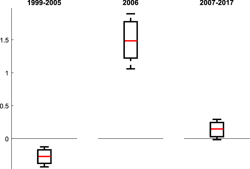
Wage bargaining shocks, quarterly averages. Red: medians, boxes: quartiles, whiskers: 16%/84%.

Also in all other robustness specifications, we find the main results on the decline of unemployment—the lack of monocausality, the positive contribution of all identified shocks, and the dominance of wage bargaining shocks—qualitatively confirmed.
5.2. The Chronology of Wage Bargaining Shocks and Hartz IV
Given the eminent role of wage bargaining shocks, we investigate their chronology in more depth to inform our understanding of the mechanisms behind them. It is useful to remember that a wage bargaining shock represents a deviation from the estimated wage setting behavior. A prevalence of positive (negative) wage bargaining shocks means that workers get a smaller (larger) fraction of total income than in similar macroeconomic circumstances in the sample period. “Positive” and “negative” refer to the the shock’s initial impact on output. Figure 4 provides a graphical summary of the prevalence of identified wage bargaining shocks. The first of three box plots shows that in the period from 1999 until and including 2005, negative wage bargaining shocks dominated. This means that on average workers were paid more than in similar macroeconomic circumstances over the full sample.

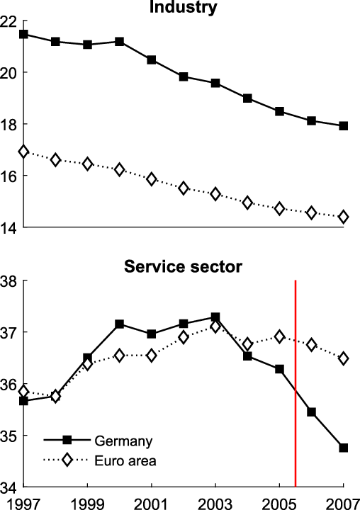
Before we discuss the prevalence of wage bargaining shocks from 2006 onwards, as visualized in the second and third box plots, we briefly investigate the evolution of wage shares in Germany and compare it to that in the entire euro area. We differentiate between industry and service sector wages as a share of the economy-wide gross value added. The upper panel of Figure 5 shows that in the decade from 1997 to 2007, industrial wage shares evolved quite similarly in the two territories. They both followed a downward trend, which was most probably owed to increased global competition and outsourcing at that time. In the service sector, wages did not trend down on average, and up to 2005 the wage share in Germany followed the one in the euro area quite closely, with no more than half a percentage point of deviation (lower panel of Figure 5). In 2006, however, German wages fell significantly short of the euro area reference value. The gap widened even further in 2007, so that the wage share of the German service sector was almost 2 percentage points lower than in the entire currency union.Footnote 7
This development is identified as a wage bargaining shock by our model: According to the second box plot in Figure 4, a strong positive wage bargaining shock hit the economy in 2006. Given the chronology of labor market reforms, it seems that Hartz IV, enacted in January 2005, has a certain stake in this outcome. While earlier reform measures, especially Hartz III, aimed at improving labor market matching, Hartz IV constituted a reduction of wage-replacement benefits. As such it reduced benefits payments for long-term unemployed and merged unemployment and social assistance (Krebs and Scheffel Reference Krebs and Scheffel2013). As an important component of Hartz IV, the unemployment benefit durations for older workers were shortened substantially. The entitlement duration was cut by more than half a year for elderly workers and by a bit less for younger workers (for more details on the reform steps, see also Hochmuth et al. Reference Hochmuth, Moyen and Stähler2019). The substantial reduction of wage-replacement benefits depressed reservation wages. This, in turn, affected wage negotiations in 2005, and ultimately dampened wage outcomes in 2006.
The (reservation) wage dampening effect of the reform obviously had different effects in different sectors. While sectoral wages as a share of sectoral output fell from 2005 to 2006 in both the manufacturing and the service sector, industrial output benefited, possibly due to enhanced competitiveness. This counteracted the wage bump so that, overall, the manufacturing wage share in total output was not noticeably affected, but rather resumed smoothly on its downward path. Conversely, the under-performance of services relative to industry and the total economy added to the wage decline in this sector so that the service wage share in total output was considerably dampened after 2005.
Note that our interpretation does not contradict the observation of Dustmann et al. (Reference Dustmann, Fitzenberger, Schönberg and Spitz-Oener2014) that competitiveness of German firms had already improved before 2005. These authors find that, as early as in the 1990s, the German manufacturing sector benefited from trade integration with Eastern Europe through cheap imported inputs, and that it did so far more than any other (Western) European country. This dampened unit labor costs of “end products” but left labor costs of value added—which is closely related to our manufacturing wage measure—unaltered (see Dustmann et al. Reference Dustmann, Fitzenberger, Schönberg and Spitz-Oener2014, panel B of Figure 4, p. 175).Footnote 8 Taken together, we think that both aspects mattered for the labor market miracle. The beneficial development in the manufacturing sector since the 1990s was an important prerequisite, while the changes due to the labor market reforms ultimately triggered the trend reversal in German unemployment.
While wage moderation was heavy in 2006, it was not limited to that year. Less dramatic but steady, it persisted from then onwards over the entire remaining sample period: As the third box plot in Figure 4 shows, in the period from 2007 to 2017 positive wage bargaining shocks dominated, pointing to persistent wage moderation in the years that followed the Hartz IV reform. From the analysis of impulses responses, we know that the reduction of wages following a wage bargaining shock is only a short-run phenomenon. In the medium run, it is reversed thanks to rising labor demand, which dampens unemployment further. This mechanism seems compelling: first pay less, then produce more, subsequently catch up with earnings, and end up with lower unemployment. But it also seems unsustainable on a national scale.
5.3. Euro Area Mechanisms
We conjecture that euro area mechanisms play a role in this regard. Hochmuth et al. (Reference Hochmuth, Moyen and Stähler2019) find that wage moderation raised the German current account significantly. Bettendorf and Leon-Ledesma (Reference Bettendorf and Leon-Ledesma2019) confirm this effect and point to different adjustment processes before and after the establishment of the EMU. In the pre-EMU period, real effects of wage moderation were offset by the appreciation of the Deutschmark. Within the monetary union, country-specific wage moderation raises (net) exports and output more persistently, as a compensating exchange rate response is not in place.
We can corroborate these differences when we estimate the model on the pre-EMU sample, that is, from 1970 to 1998: According to the impulse responses, wage bargaining and matching efficiency shocks affect the unemployment rate in the pre-EMU regime much less persistently than in the entire sample (cf. Figure A6 in the Appendix). In the estimation over the entire sample, the unemployment rate remains significantly below its pre-shock level even 5 years after the impact of a wage bargaining shock. When estimation is restricted to the pre-EMU sample, its decline is fully offset. Also for matching efficiency shocks, the unemployment decline is purely transitory in the pre-EMU regime, while it is more persistent over the entire sample. Equivalent but less pronounced results hold for output.
This means that real effects of autonomous labor market shocks are more persistent since the introduction of the common currency than they were before. One might wonder whether price adjustments can compensate for the exchange rate mechanism, that is, whether “external appreciation” is replaced by “internal appreciation”. Our results suggest that this is not the case. In the entire sample, prices respond even less to the positive demand repercussions of wage moderation than in the pre-EMU period. This might explain why wage moderation in Germany was so persistent: Absent exchange rate adjustments, both firms and workers have benefited from wage moderation, because higher demand for German products lifted profits and dampened unemployment.
5.4. The Role of Wage Bargaining Shocks
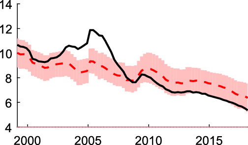
Given the importance of wage bargaining shocks for the German labor market miracle, we want to know how the unemployment rate would have evolved in their hypothetical absence. Figure 6 presents the realized unemployment rate and the range of its hypothetical counterfactuals. In 1999, the effect of wage bargaining shocks on unemployment, that had accumulated since 1970, was negative according to most draws. The gap widened until 2005 because a series of negative wage bargaining shocks hit the economy. Thus, in the first years after the millennium, tight wage negotiations put an upward pressure on salaries which led to increases in the unemployment rate. In 2006, negative wage bargaining shocks started to materialize and dampened unemployment. At the time of the Great Recession, their cumulative effects were largely compensated. From then onwards, small but steady positive wage bargaining shocks kept dragging unemployment down. In the absence of wage bargaining shocks, the unemployment rate would be up to 2 percentage points higher at the end of the sample.
Counterfactual unemployment rate excluding wage bargaining shocks. Black: data, red: counterfactuals (dotted: median, area: quartiles).

Two other observations are worthwhile to mention: First, the jump of unemployment in 2005 (by approximately 1 percentage point) was not due to wage bargaining shocks. Instead, according to our model, it was to a large extent due to a labor supply shock. We attribute this labor supply shock to the effects of Hartz IV. Certain groups of the population, who were not eligible for pre-reform benefits, registered for unemployment under the new regime because they were eligible for post-reform benefits; including in particular young adults up to the age of 25 (Brenke Reference Brenke2010). Beyond that, municipalities had a strong interest in declaring as many pre-reform welfare recipients as possible fit for work, because it made them eligible for the post-reform benefits which were financed by the federal government. Burda and Seele (Reference Burda and Seele2016) confirm that the Hartz reforms raised labor supply, in particular in West Germany.Footnote 9
The second observation worthwhile to mention is that wage bargaining shocks, while accounting for much of the secular decline of unemployment, are not related to its small hike during the Great Recession. We focus on this second part of the German labor market miracle in the following section.
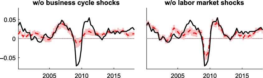
Counterfactual y-o-y GDP growth rate. Black: data, red: counterfactuals (dotted: median, area: quartiles).

6. The Labor Market Miracle, Part II
The second part of the German labor market miracle concerns the increase of unemployment during the Great Recession which was exceptionally low given the large output loss. While GDP dropped by almost 5% in the first quarter of 2009, the maximum quarterly loss in the USA was 2%. Meanwhile, unemployment soared from below 5% in the USA before the crisis to almost 10% thereafter, while in Germany it increased only temporarily and by less than 1 percentage point. Hence, the negative spillovers from real activity to unemployment appear marginal, and the decline of unemployment persisted beyond the Great Recession.
To investigate this issue in more details, we summarize the five structural shocks of our VAR into two broad categories: business cycle shocks, consisting of aggregate demand and technology shocks, and labor market shocks, comprising labor supply, wage bargaining, and matching efficiency shocks. This allows us to approach this part of the labor market miracle in the following way: First, we construct GDP growth counterfactuals to show that the Great Recession (and the ensuing recovery) were pure business cycle phenomena, that did not originate from the labor market. Second, we compare forecast error variance decompositions of GDP and the unemployment rate for Germany and for the USA. We find that they are almost identical for GDP but substantially different for unemployment. This leads us, third, to investigate the intensive margin of labor in more detail and its response to business cycle shocks, to which end we extend the model to incorporate also the intensive margin, namely hours worked.
6.1. The Great Recession as a Business Cycle Phenomenon
In a first step, we conduct a counterfactual analysis of GDP growth to investigate which shocks contributed to its strong decline during the Great Recession. According to our model, the Great Recession was indeed a business cycle phenomenon: In 2009, GDP would have hardly declined in the absence of business cycle shocks (left panel of Figure 7), while absent labor market shocks the drop would have been practically unaltered (right panel).Footnote 10 The figure also shows that the same applies to the recovery that followed the Great Recession: It constituted a cyclical recovery primarily driven by business cycle innovations. Without strong positive impulses from business cycle shocks, GDP growth over the period 2009–2012 would have been at most subdued, but it would not have fluctuated as heavily as it actually did.
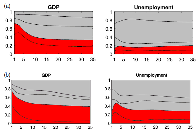
FEVDs of GDP and unemployment. (a) Germany, own calculations; (b) USA, based on Foroni et al. (Reference Foroni, Furlanetto and Lepetit2018). Red: business cycle shocks, gray: labor market shocks.

The recession was not only followed by an expansion but it was also preceded by a period of above-average growth rates. This preceding expansion was very different in kind compared to the recovery: According to the counterfactuals in Figure 7, the growth acceleration before the crisis was largely a labor market phenomenon that kicked in around 2005 when the Hartz IV reform measures were implemented. There were hardly any business cycle impulses to GDP growth. Indeed, business sentiment indicators were muted in the years preceding the Great Recession, as observed by Burda and Hunt (Reference Burda and Hunt2011). But while these authors argue that there was a business cycle surprise contrary to firms’ expectations (so that firms hired fewer workers and, hence, had to fire fewer during the recession), we find that firms’ expectations were perfectly in line with what we identify as a weakness of the business cycle. If growth had surprised firms back then, it was growth emanating from shocks originating from the labor market. This, not a wrong assessment of the stance of the business cycle, explains the evolution of the unemployment rate prior, during, and following the crises, which we show in a next step by means of forecast error variance decompositions.
6.2. The Relevance of the Business Cycle across Countries and Time
We have already conducted a forecast error variance decomposition (FEVD) and compared it to the results of Foroni et al. (Reference Foroni, Furlanetto and Lepetit2018) for the USA. In this section, we first rearrange the results to highlight the similarities and the substantial differences between the two countries. Then we compare the full-sample behavior of forecast error variances with results for a sample excluding the Great Recession.
In the upper panels of Figure 8, the forecast error variance decompositions for output and the unemployment rate are reproduced with different colors such that the broad categories of business cycle shocks (red) and labor market shocks (gray) can be distinguished. The lower panels show the corresponding graphs from Foroni et al. (Reference Foroni, Furlanetto and Lepetit2018) for the USA. Forecast error variances of output share remarkably similar structural patterns. In both countries, business cycle shocks are the most important short-run drivers of output, accounting for three quarters of the respective forecast errors. In the medium run, the relevance of business cycle shocks declines.
The results are very different for the unemployment rate. In the USA, business cycle shocks play a much larger role for unemployment fluctuations than in Germany. This is true for all horizons, but particularly in the short run, where business cycle shocks account for up to a half of the forecast error variance in the USA. In the medium term, its relevance declines to a quarter. In Germany, in contrast, it never reaches such a high value. It accounts for at most a fifth of the unemployment forecast error variance. Importantly, business cycle shocks do not account for a higher unemployment forecast error in the short run than in the medium run. These differences are particularly relevant as output forecast error variances behave so similarly. We conclude from this observation that the adjustment of labor input to business cycle induced output variation is weak on the extensive margin in the German economy. As a result, the small increase in unemployment during the Great Recession should be interpreted as the combination of a severe business cycle shock that triggered the marked decline of GDP and the limited spillovers from GDP growth to unemployment.
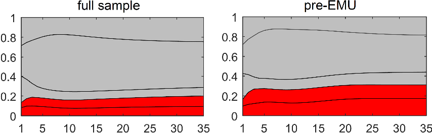
We now turn to the question, whether the muted response of unemployment to business cycle fluctuations in Germany was different prior to the Great Recession, that is, whether the Great Recession was an exceptional event that drives the results. To answer this question, we resort to the model estimated on the pre-EMU sample. The contributions of business cycle and labor market shocks to the unemployment forecast error variance for this sample are presented in the right panel of Figure 9 along with the results for the full sample in the left panel. In the pre-EMU sample, business cycle shocks accounted for a larger fraction of the unemployment forecast error variance than in the full sample, implying that the response of unemployment to the business cycle became more muted in the last two decades. Still, its contribution in the pre-EMU sample was at most a quarter, both in the medium and in the short run.
FEVDs of German unemployment, different samples. Red: business cycle shocks, gray: labor market shocks.

In sum, unemployment in Germany appears to have increased by less during the Great Recession than during earlier downturns relative to the size of the recessions in terms of output loss. However, also more generally the short-run response of unemployment to business cycle fluctuations is much more muted in Germany than in the USA, and had been so already in former times. We conjecture that this is due to circumstances, institutions or characteristics that are inherent to the German economy, in particular short-time work arrangements.
Indeed, existing research on the effects of short-time work is consistent with these observations. Based on German data and a VAR approach, Balleer et al. (Reference Balleer, Gehrke, Lechthaler and Merkl2016) show that short-time work is effective in mitigating job losses in response to output shocks (that is, business cycle shocks) and that it dampens unemployment. Employing a non-linear VAR, Gehrke and Hochmuth (Reference Gehrke and Hochmuth2021) find that also discretionary changes of short-time work arrangements have the desired effects on labor market outcomes, when they are introduced in recessions. Given that short-time work was considerably expanded during the Great Recession, they argue that this discretionary component reinforced the dampening effects on unemployment brought about by its systematic part. Brey and Hertweck (Reference Brey and Hertweck2020), Cooper et al. (Reference Cooper, Meyer and Schott2017), Boeri and Bruecker (Reference Boeri and Bruecker2011) and others arrive at similar conclusions.
The comparably small response of the extensive margin of labor to the business cycle raises the question of whether and to which extent the intensive margin adjusts. We explore this in the third and final step of this analysis. It turns out that the intensive margin is indeed an important cushion to business cycle fluctuations.
6.3. The Intensive Margin
So far, our analysis focused on changes in the extensive margin and we provided evidence that aggregate demand and technology shocks have only a modest impact on unemployment in Germany. However, also the intensive margin adjusts to economic innovations. The small increase in the unemployment rate during the Great Recession might be explained by a comparably stronger adjustment in hours worked. Consequently, the question arises of how hours worked respond to the identified structural shocks of our model. To investigate this issue, we re-estimate the baseline model and include log hours worked per capita in the set of variables. Adding this variable to the model generates another equation and, hence, another orthogonal shock. We leave this shock unidentified (“residual shock”).
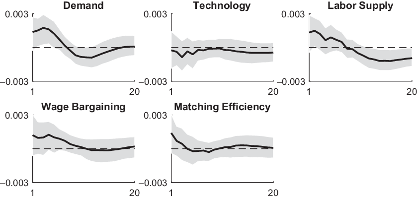
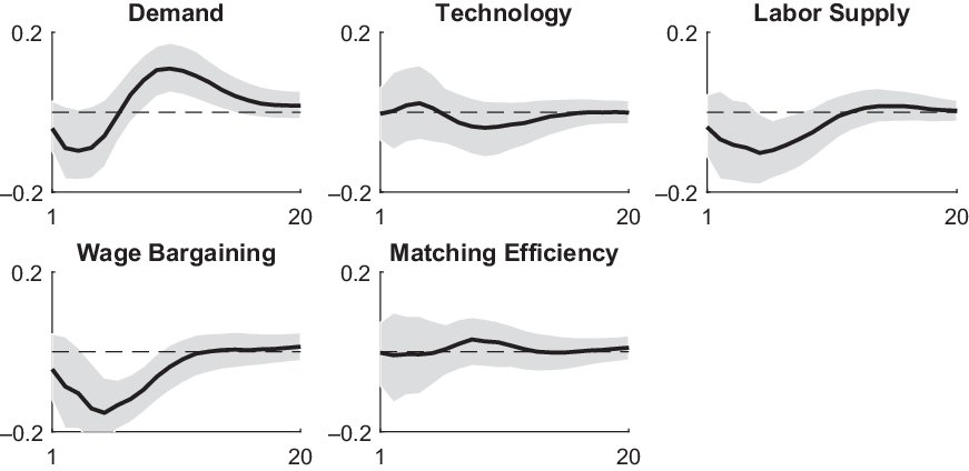
For each identified structural shock, the response of hours worked is left unrestricted, so we impose the same set of restrictions as in the 5-variable baseline model. The impulse responses of hours worked are presented in Figure 10, and the full set of impulse responses of the 6-variable VAR is provided in the Appendix (Figure A5). In spite of not imposing additional sign restrictions we observe that, on impact, per capita hours worked co-move positively with total output except for technology shocks. The share of draws that exhibit an impact increase of per capita hours worked in all valid draws amounts to 80% for aggregate demand shocks, 78% for matching efficiency shocks, 77% for labor supply shocks, 73% for wage bargaining shocks, and 44% for technology shocks.
Impulse responses of per capita hours worked to various shocks. Note: medians and corresponding 68% credible sets.

These results corroborate some aspects of a model recently put forward by Cacciatore et al. (Reference Cacciatore, Fiori and Traum2020). They introduce adjustment costs for hours worked and non-separable preferences in an otherwise standard New-Keynesian business cycle model with search-and-matching frictions to allow for greater flexibility with regard to the “wealth effect” (i.e. the degree of substitution between leisure and work) on labor supply decisions. Our results confirm the following three aspects of their model. First, hours worked respond procyclically to aggregate demand shocks. Second, they respond only modestly and on average countercyclically to technology shocks. Third, hours worked respond procyclically to labor supply shocks. With regard to wage bargaining shocks, the response of the intensive margin is dampened in the model of Cacciatore et al. (Reference Cacciatore, Fiori and Traum2020) compared to the standard model with costless hours adjustment and additively separable preferences. It remains countercyclical though, something that we cannot confirm from our empirical results. Instead, wage bargaining shocks and matching efficiency shocks elicit a positive co-movement of the intensive margin and output.
Figure 11 presents the contributions of business cycle and labor market shocks (and the residual shock) to the forecast error variance of unemployment and hours worked. It shows that business cycle shocks explain more of the unexplained variation of the intensive margin than of the extensive margin. The bulk of labor adjustment in response to business cycle shocks occurs at the intensive margin. This explains the modest reaction of German unemployment during the Great recession in contrast to the sizable response of per capita hours worked.
FEVDs, 6-variable VAR including hours worked. Red: business cycle shocks, gray: labor market shocks, white: residual shock.

The counterfactual analysis (Figure 12) corroborates this finding. What is more, counterfactual per capita hours evolved very similarly to counterfactual GDP growth: The pre-recession increase is identified as originating from the labor market, while the decline in 2009 and the ensuing recovery where driven by the business cycle. Unemployment, on the other hand, was almost entirely driven by labor market shocks over the last two decades. Without labor market shocks, it would have evolved substantially flatter. This reinforces the evidence that in Germany the intensive margin of labor is the primary cushion of business cycle variations, that is, that it is much more responsive to demand and technology shocks than the extensive margin.
Counterfactuals excluding labor market shocks. Black: data, red: counterfactuals (dotted: median, area: quartiles).

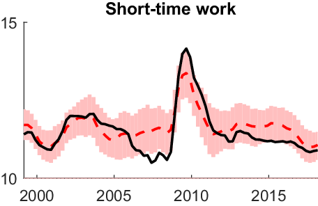
The policy instrument of short-time work appears to be essential in this regard. To corroborate this presumption, we re-estimate the 6-variable VAR replacing hours worked with the number of short-time workers. The time series of this variable displays a clear (counter-)cyclical pattern (Figure A2). This pertains to its response to the identified structural shocks (Figure A4): It decreases when output goes up, be it as immediate effect to an aggregate demand shock or as a lagged response to labor supply and wage bargaining shocks. On the other hand, short-time work does not respond systematically to technology-induced shocks, that is, general and matching-specific technology shocks. Counterfactual short-time work absent labor market shocks shares strong similarities with counterfactual hours (Figure 13). In particular, the jump during (and the leveling off after) the Great Recession was business cycle driven, while the reduction in the pre-crisis years emanated from labor market-specific shocks.
STW counterfactual excluding labor market shocks. Black: data, red: counterfactuals (dotted: median, area: quartiles).

To summarize, our findings imply that movements in the extensive margin in Germany are mainly driven by labor market shocks. Especially wage bargaining shocks are responsible for the persistent and strong decline in unemployment that started in 2005. In contrast, changes in the intensive margin are driven by both business cycle and labor market innovations. The strong adjustment of the intensive margin during the Great Recession helped to keep the rise in unemployment low. Short-time work regulations anchored in German labor law might have played a certain role. By subsidizing wages, they encouraged firms which are forced to reduce labor input to do so on the intensive rather than on the extensive margin.
7. Conclusion
In this article, we study the macroeconomic driving forces of the German labor market miracle, which includes (i) the strong decline of unemployment since 2005 and (ii) the small increase of unemployment during the Great Recession. We contribute to the existing literature by gauging the impact of various factors within a consistent macroeconometric framework. In particular, we estimate VARs on quarterly German data and identify different business cycle and labor market shocks based on robust sign restrictions.
Our results indicate that the decline of unemployment was not monocausal, but that wage moderation was the dominant driver. The effect of wage bargaining shocks was particularly pronounced right after the implementation of Hartz IV, which reduced wage replacement benefits and, hence, the reservation wage. Improved matching efficiency, targeted by other reform measures, also contributed to the decline of unemployment.
We also identify shocks that are not related to labor market policy reforms. In particular, a shortage of labor supply helped to bring unemployment down. While the Hartz reforms raised labor supply, other developments must have pushed it in the opposite direction, for example demography. So far, however, studies on the unemployment effects of the shrinking working-age population in Germany are rare (e.g. Fuchs Reference Fuchs2016). This issue might provide a promising area for future research.
We also find that wage moderation was not limited to the immediate aftermath of the implementation of Hartz IV, but that it persisted far beyond the reform and the Great Recession. It seems that trade unions perceived wage moderation as a worthwhile strategy because of its beneficial medium to long run effect on unemployment and wages. The sustainability of this effect is hard to reconcile on a national level and our results show that since the implementation of the monetary union the positive real effects of country-specific wage moderation strengthened.
With respect to the Great Recession, we find that the small impact of business cycle shocks at the extensive margin of labor is an inherent feature of the German economy and likely related to favorable labor market institutions such as short-time work arrangements. This presumption is based on the finding that the intensive margin (hours worked per capita) is a more important cushion for business cycle fluctuations than the extensive margin. Rather than firing and hiring staff in downturns and upturns, German firms vary the working time of their workers in response to business cycle fluctuations. Apart from the unemployment smoothing effect, this labor hoarding might also help firms preserving human capital.
Acknowledgements
We are grateful for helpful comments from two anonymous referees on the previous version of this paper. Moreover, we thank Fabio Canova, Marius Clemens, Francesco Furlanetto, Martin Kerndler, Christian Merkl, Roland Winkler, and participants of the 2019 WU-Workshop in Applied Econometrics, the 2019 CEF International Conference, the 2019 VfS Annual Conference, and the 2020 NOeG Annual Meeting for helpful comments and suggestions and Maria Riegler for excellent research assistance. The opinions expressed in this article are the sole responsibility of the authors and should not be interpreted as reflecting the views of Sveriges Riksbank.
A. Appendix
Further aspects of unemployment. (a) Registered vs. survey-based rate harmonized along ILO definitions; (b) Unemployment rates in West and East Germany; (c) Total number of unemployed (left axis) subdivided into gender (right axis).

Data. Notes: Inflation measured as y-o-y change of log CPI (black) and of log GDP deflator (gray); log real wages per capita (black) and per hour (gray); unemployment rate: registered (black) and harmonized (gray, extended with the registered rate before 1995). All data of West-Germany before reunification. All data seasonally adjusted except for CPI. Sources: Destatis, OECD, Federal Employment Agency, Gehrke and Hochmuth (Reference Gehrke and Hochmuth2021).

Robustness #1:
 $l=3$
with baseline (
 $l=5$
) credible sets.

Robustness #2:
 $l=7$
with baseline (
 $l=5$
) credible sets.

Robustness #3: CPI replaced by GDP deflator, baseline credible sets.

Robustness #4: wages per capita replaced by wages per hours worked, baseline credible sets.

Pre-EMU (1970–1998) median responses, baseline credible sets.

Impulse responses, 6-variable VAR with hours worked.

Impulse responses of short-time work.