1 Introduction
Stably stratified fluids are found throughout nature in lakes, ponds, oceans, the atmosphere and even in the Sun. For example, apart from the upper layer and isolated regions, the ocean is generally stably stratified; the vertical density gradient, measured from the ocean floor, is negative while the vertical temperature gradient, if any, is positive (Staquet Reference Staquet2005). This stable stratification is prevalent in isolated environments such as pores and fractures where mixing is negligible, and can lead to intense biological activities and accumulation of particles and organisms (MacIntyre et al. Reference MacIntyre, Romero, Silsbe and Emery2014).
In engineering, stable stratification can be utilized for heat and mass transport problems, such as cooling of nuclear reactors (Zhao & Peterson Reference Zhao and Peterson2010) and energy generation from solar ponds (Lin Reference Lin1982). Stratification plays an important role in engineering design and analysis of submerged objects since density variations in the fluid may influence the object’s motion. A notable example is the ‘dead-water’ phenomenon (Maas & van Haren Reference Maas and van Haren2006), where a boat on the surface experiences an increase in drag due to low-pressure build up behind it from internal waves being generated along the interface of two-layer stratified fluids (Mercier, Vasseur & Dauxois Reference Mercier, Vasseur and Dauxois2011). This phenomenon exists when a layer of lower-density fluid, such as fresh water, overlies higher-density fluid, such as sea water, at the mouth of a river or near melting glaciers. In swimmers, Ganzevles et al. (Reference Ganzevles, van Nuland, Maas and Toussaint2009) found that swimming strokes are less efficient in stratified fluid and swimming speeds are slower by as much as 15 %. Enhanced drag was also observed in horizontally moving spheres by Lofquist & Purtell (Reference Lofquist and Purtell1984) and later by Lin, Boyer & Fernando (Reference Lin, Boyer and Fernando1992a ) and Lin et al. (Reference Lin, Lindberg, Boyer and Fernando1992b ), with changes in the drag coefficient being a function of the stratification level. While most studies focused on horizontal motion in stratified fluids, similar changes in behaviour have been observed in vertically moving objects (see Torres et al. Reference Torres, Ochoa, Castillo and Hanazaki1999, Reference Torres, Hanazaki, Ochoa, Castillo and Van Woert2000; Hanazaki, Kashimoto & Okamura Reference Hanazaki, Kashimoto and Okamura2009; Yick et al. Reference Yick, Torres, Peacock and Stocker2009; Camassa et al. Reference Camassa, Falcon, Lin, McLaughlin and Mykins2010; Doostmohammadi, Dabiri & Ardekani Reference Doostmohammadi, Dabiri and Ardekani2014). For example, Torres et al. (Reference Torres, Ochoa, Castillo and Hanazaki1999) found an increase in drag on a sphere settling in a stably stratified fluid due to a buoyant jet forming behind the sphere.
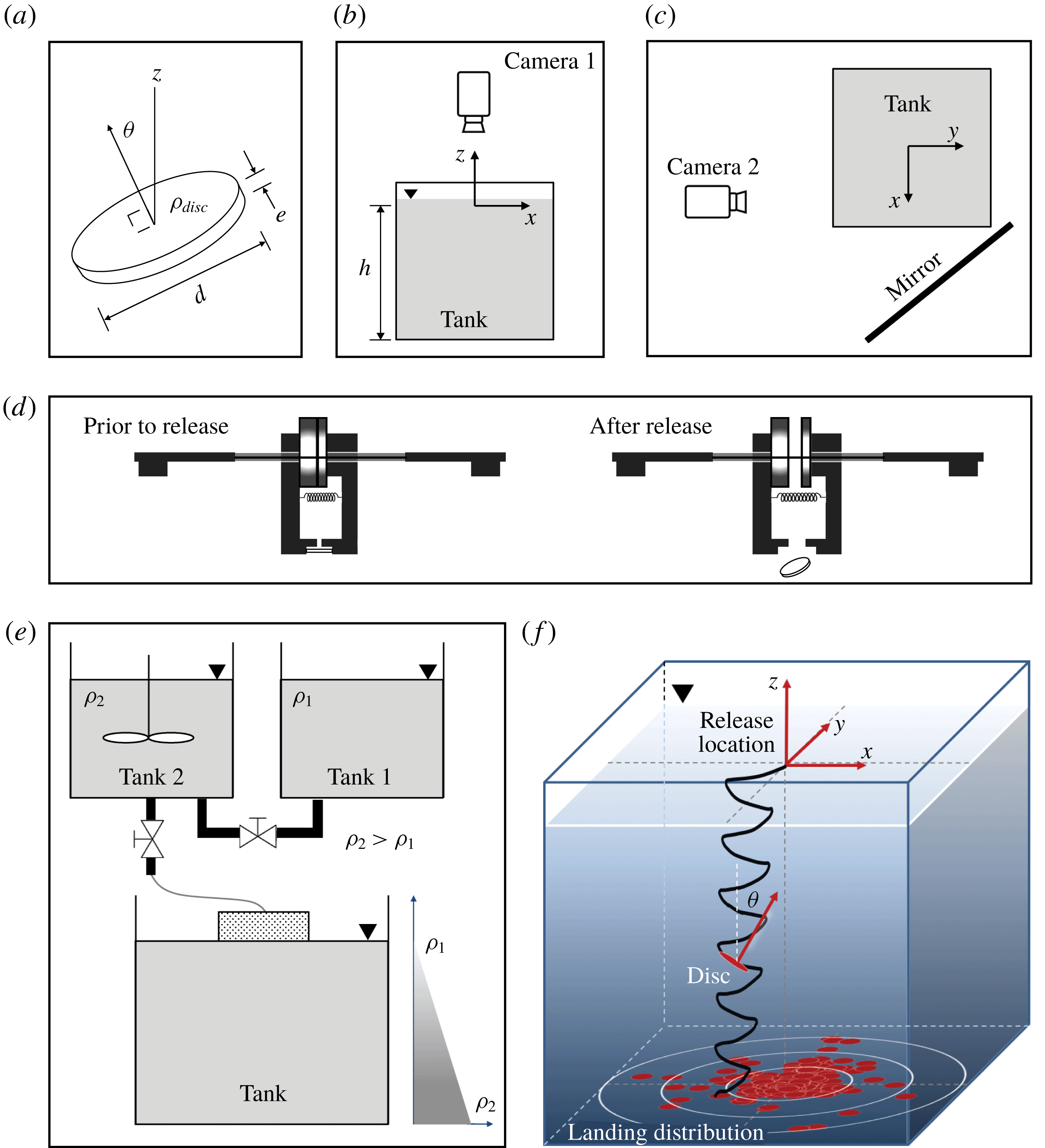
(a) Disc of diameter
 $d$
, thickness
 $e$
and density
 $\unicode[STIX]{x1D70C}_{disc}$
at an inclination angle
 $\unicode[STIX]{x1D703}$
defined as the angle between the vertical
 $z$
-direction and the normal to the disc. (b,c) Side and top views of the experimental set-up used to record the disc’s landing location and 3D trajectory, respectively; the mirror in (c) captures an orthogonal view necessary for 3D reconstruction. (d) Electromagnet release mechanism prior to release with the disc and after the disc is released. (e) Two-tank experimental free-drained set-up used to generate a stable linear density profile in the tank. (f) Schematic of the tank set-up with a sample reconstructed trajectory. The coordinate system is centred at the initial release location. The landing locations for multiple consecutive drops are shown in red and used to compute the landing distribution.

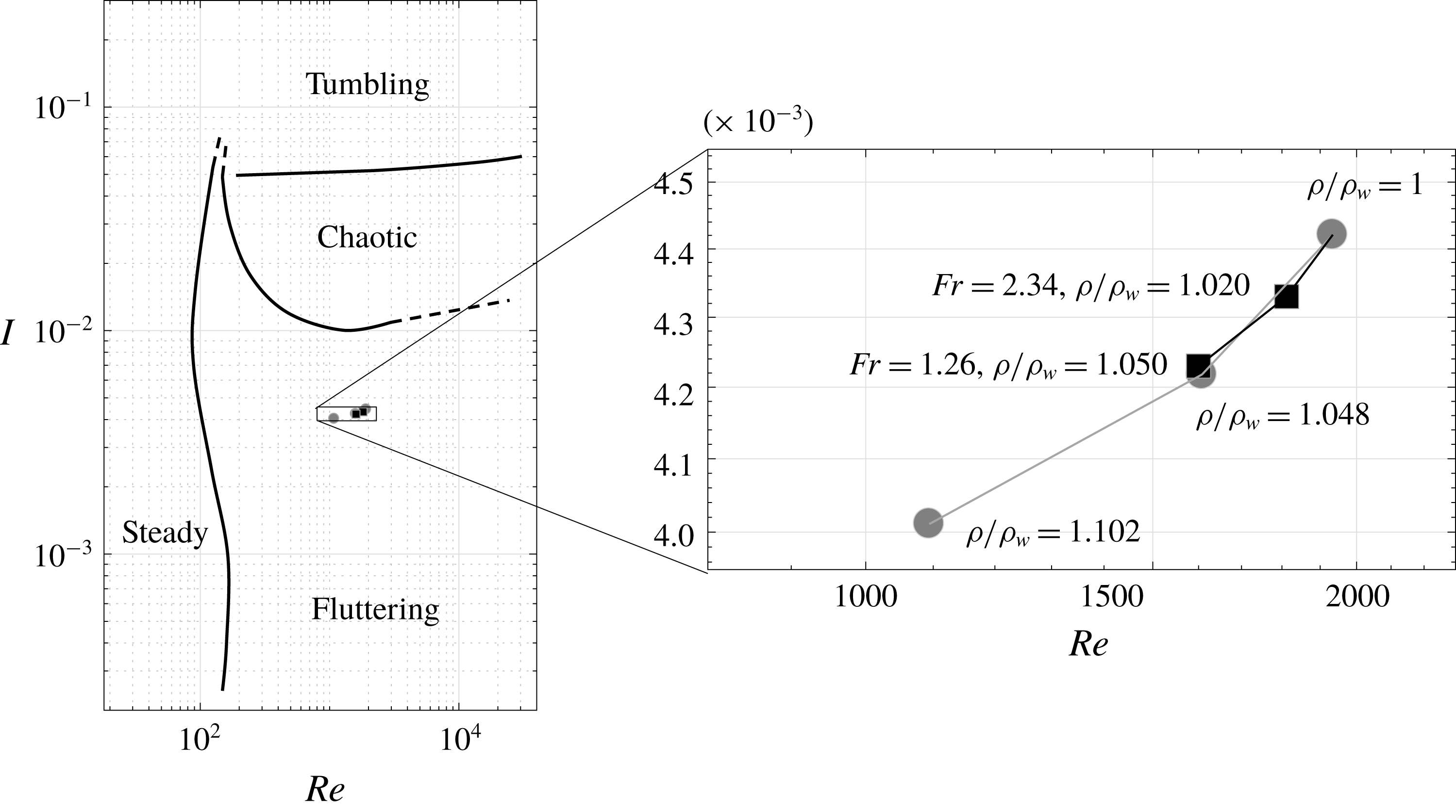
Discs freely falling in homogeneous fluids belong to one of four descent regimes: steady, fluttering, chaotic or tumbling. These regimes are mapped onto the parameter space (
 $Re,I$
) based on the results of Field et al. (Reference Field, Klaus, Moore and Nori1997). The parameter values explored in this paper are highlighted: constant density fluid (○) consisting of pure water
 $\unicode[STIX]{x1D70C}/\unicode[STIX]{x1D70C}_{w}=1$
, saltwater density values
 $\unicode[STIX]{x1D70C}/\unicode[STIX]{x1D70C}_{w}=1.048$
and
 $\unicode[STIX]{x1D70C}/\unicode[STIX]{x1D70C}_{w}=1.102$
and stratified saltwater fluid (▫) at two levels of stratification
 $Fr=2.34$
and
 $1.26$
. For stratified fluids, we computed
 $I$
and
 $Re$
using the average density values.

In this paper, we experimentally investigate the motion of rigid discs falling freely in a vertically stratified fluid of saltwater solution (figure 1). Even without stratification, the fluid–structure interactions lead to rich descent dynamics that have attracted the attention of scientists since the early observations of Maxwell in 1853 (Maxwell Reference Maxwell1990). In homogenous fluids (constant density), the descent motion depends on the Reynolds number
 $Re$
and the dimensionless moment of inertia
 $I$
of the falling object. The Reynolds number is defined as
 $Re=\unicode[STIX]{x1D70C}Ud/\unicode[STIX]{x1D707}$
, where
 $d$
and
 $U$
are the diameter and terminal velocity of the disc while
 $\unicode[STIX]{x1D70C}$
and
 $\unicode[STIX]{x1D707}$
are the density and viscosity of the fluid, respectively. We estimate the disc’s terminal speed as the speed at which the disc’s weight balances buoyancy and drag forces. We obtain
 $U=\sqrt{2eg|\unicode[STIX]{x1D70C}_{disc}/\unicode[STIX]{x1D70C}-1|/C_{D}}$
, where
 $\unicode[STIX]{x1D70C}_{disc}$
is the density of the disc,
 $e$
its thickness and
 $g$
is the gravitational constant equal to
 $g=9.81~\text{m}~\text{s}^{-2}$
(see figure 1
a). In calculating
 $U$
, we set the drag coefficient to
 $C_{D}=1.2$
, consistent with the value for a disc normal to a uniform flow (see Hoerner Reference Hoerner1965). The dimensionless moment of inertia is given by
 $I=\unicode[STIX]{x03C0}\unicode[STIX]{x1D70C}_{disc}e/64\unicode[STIX]{x1D70C}d$
. Based on
 $(Re,I)$
, the descent motion of the disc falls into one of four main descent regimes: steady, fluttering, tumbling or chaotic. In figure 2, we map the four descent regimes onto the phase space
 $(Re,I)$
based on the results of Field et al. (Reference Field, Klaus, Moore and Nori1997).
Starting from the fluttering regime, we systematically vary the fluid environment in order to examine the effect of changes in the fluid density on the fluttering behaviour. In particular, we consider three fluid environments: pure water, constant-density saltwater (larger than that of pure water) and stratified saltwater (density varying linearly from pure water to saltwater). We choose the parameters carefully so that in all three environments,
 $(Re,I)$
lies robustly in the fluttering regime, as detailed in the inset of figure 2. We reconstruct the descent trajectories and orientation of the fluttering disc and we analyse the effect of stratification on the descent behaviour. We find that stratification significantly decreases the vertical descent speed, fluttering amplitude and inclination angle of the disc, while simultaneously increasing its radial dispersion (horizontal distance from drop location). Our findings are consistent but go beyond current numerical and experimental observations of two-dimensional ellipses in stratified fluids (Hurlen Reference Hurlen2006).
This paper is organized as follows. A brief overview of the literature on passive flight in homogenous fluids is presented in § 2. A description of the experimental methods is given in § 3. The resulting experimental observations are presented in § 4. In § 5, we discuss the physical mechanisms underlying these observations. Based on these mechanisms, we formulate in § 6 a two-dimensional quasi-steady model that include forces and moments that arise from density stratification. Taken together, the experimental results and analytical model explain how density stratification decreases the vertical descent speed, fluttering amplitude and inclination angle of the disc. In § 7, we probabilistically examine the effect of stratification on the radial dispersion of the disc by comparing the probability distribution function (p.d.f.) of landing sites in density-stratified fluid to that in pure water. We find that stratification enhances radial dispersion. We conclude in § 8 by commenting on the relevance of these results to engineering and biological applications.
2 Overview of passive flight in homogeneous fluids
We briefly review the literature on objects freely falling in homogeneous fluids. Willmarth, Hawk & Harvey (Reference Willmarth, Hawk and Harvey1964) were the first to experimentally construct a phase diagram (
 $Re,I$
) that clearly showed the transition from steady to unsteady (fluttering and tumbling) descent motions. Stringham, Simons & Guy (Reference Stringham, Simons and Guy1969) performed similar experiments with spheres, cylinders and discs, and focused on computing drag coefficients on the descending objects for a wide range of Reynolds numbers. The phase space of Willmarth et al. (Reference Willmarth, Hawk and Harvey1964) was later refined in Field et al. (Reference Field, Klaus, Moore and Nori1997) to include the boundaries between the fluttering, chaotic and tumbling regimes (see the left panel of figure 2).
Numerical investigations of thin discs and cards falling freely in a homogeneous fluid were conducted by Pesavento & Wang (Reference Pesavento and Wang2004), Andersen, Pesavento & Wang (Reference Andersen, Pesavento and Wang2005a ,Reference Andersen, Pesavento and Wang b ), Jin & Xu (Reference Jin and Xu2008), Auguste, Magnaudet & Fabre (Reference Auguste, Magnaudet and Fabre2013) and Chrust, Bouchet & Dušek (Reference Chrust, Bouchet and Dušek2013). In addition, Pesavento & Wang (Reference Pesavento and Wang2004) and Andersen et al. (Reference Andersen, Pesavento and Wang2005a ,Reference Andersen, Pesavento and Wang b ) formulated quasi-steady force models similar to those in Tanabe & Kaneko (Reference Tanabe and Kaneko1994) and Belmonte, Eisenberg & Moses (Reference Belmonte, Eisenberg and Moses1998). The associated nonlinear dynamics was analysed in Kuznetsov (Reference Kuznetsov2015), showing the existence of fixed points, limit cycles, attractors and bifurcations. Jin & Xu (Reference Jin and Xu2008) used a moving mesh method for the Navier–Stokes equations and showed good agreement between experimental and computational trajectories, while clarifying some discrepancies noted in Andersen et al. (Reference Andersen, Pesavento and Wang2005a ). Jones & Shelley (Reference Jones and Shelley2005) and Michelin & Smith (Reference Michelin and Smith2009) used low-order representations of the fluid in the context of the inviscid vortex sheet and unsteady point vortex models to shed light into the role of vorticity in destabilizing the descent motion.
Auguste et al. (Reference Auguste, Magnaudet and Fabre2013) numerically explored the parameter space (
 $Ar,I$
), where the Archimedes number
 $Ar$
is proportional to
 $Re$
. They focused on the range
 $Re<300$
(
 $Ar<110$
) and identified non-planar sub-regimes of the fluttering and tumbling regimes, which they referred to as hula-hoop (gyrating while fluttering) and helical autorotation (helical tumbling). Chrust et al. (Reference Chrust, Bouchet and Dušek2013) used non-dimensional mass and the Galileo number
 $G$
, expressed as
 $Ar=\sqrt{3/4\unicode[STIX]{x03C0}}G$
, and focused on the range of
 $G<500$
. In our experiments,
 $G>750$
and
 $Ar>366$
.
Experimentally, the hula-hoop behaviour was investigated by Zhong et al. (Reference Zhong, Lee, Su, Chen, Zhou and Wu2013) using dye visualization and particle image velocimetry (PIV) to highlight the fluid–structure interactions in these fluttering motions. Lee et al. (Reference Lee, Su, Zhong, Chen, Zhou and Wu2013) looked at transitions from two-dimensional fluttering to spiral motions and noted a critical dimensionless moment of inertia
 $I$
where the transition occurs. Heisinger, Newton & Kanso (Reference Heisinger, Newton and Kanso2014) dropped discs repeatedly in water to determine the p.d.f. associated with the landing positions in each of the four descent modes (steady, fluttering, chaotic and tumbling). Vincent, Shambaugh & Kanso (Reference Vincent, Shambaugh and Kanso2016) investigated the falling behaviour of annular discs in the (
 $Re,I$
) parameter space and found that the central hole stabilizes the descent motion of the disc.
3 Methods
To create linear density stratification in the lab, we used the two-tank method proposed by Fortuin (Reference Fortuin1960) and Oster (Reference Oster1965). This method is used widely owing to its simplicity and robustness (Hill Reference Hill2002; Spedding Reference Spedding2002; Economidou & Hunt Reference Economidou and Hunt2009). Fluid from a pure water tank and a saltwater tank is free-drained into a third reservoir as shown in figure 1(e).
In all experiments, we used a single acrylic disc of density
 $\unicode[STIX]{x1D70C}_{disc}=1143.7~\text{kg}~\text{m}^{-3}$
, diameter
 $d=2.54$
cm and thickness
 $e=2$
mm (see figure 1
a), leading to a dimensionless moment of inertia
 $I=0.00442$
. We considered a 60-gallon cubic acrylic tank of dimension 0.60 m on each side. We released the disc just below the surface of the fluid using an electromagnetic release mechanism (figure 1
d). In all experiments, the disc was initially horizontal and was released with zero initial conditions, barring small uncertainty introduced by the release mechanism. To determine this uncertainty, a heavy disc made of steel was released in air ten times. The location of the disc when it reached the bottom of the tank was recorded with a top-mounted camera (figure 1
b). To prevent the disc from sliding after landing, a grid mesh was added to the bottom of the tank. The standard deviation of the landing position in air was found to be less than 1.5 % of the descent height
 $h$
. In recording these data points, it was convenient to introduce a Cartesian coordinate system
 $(x,y,z)$
with origin located at the site of the release mechanism and
 $z$
-axis pointing vertically upward (figure 1
f).
Key dimensional and non-dimensional parameters explored in this paper. An average fluid density value is used to compute quantities for the stratified cases. Here
 $U$
is the terminal speed where the weight is balanced by buoyancy and drag forces.

In each experimental trial, the disc travelled a vertical distance
 $h=0.53$
m to reach the bottom of the tank. We recorded the descent motion using a high-resolution monochrome digital video camera (Point Grey Grasshopper3) set to a moderate frame rate (30–50 fps). A properly positioned mirror was used to simultaneously capture a side view of the disc for 3D reconstruction purposes (figure 1
c). The position
 $(x,y,z)$
of the centre of the disc and its orientation represented by the direction of the unit vector
 $\boldsymbol{n}$
normal to the disc were reconstructed directly from the high-speed photography using an in-house image processing algorithm (Heisinger et al.
Reference Heisinger, Newton and Kanso2014; Vincent et al.
Reference Vincent, Shambaugh and Kanso2016). The instantaneous velocity was determined by taking the time difference between consecutive frames. Successive descents are approximately 10 min apart or longer to ensure that the fluid returns to a quiescent state.
We considered three fluid environments: (i) pure water with uniform density
 $\unicode[STIX]{x1D70C}_{w}=1000~\text{kg}~\text{m}^{-3}$
; (ii) constant-density saltwater obtained by uniformly increasing the salt concentration, using salt with
 ${\geqslant}99.5\,\%$
NaCl; (iii) density-stratified fluid obtained by linearly increasing salinity with depth, with density gradient
 $\unicode[STIX]{x1D6FE}=\text{d}\unicode[STIX]{x1D70C}/\text{d}z<0$
and density profile
 $\unicode[STIX]{x1D70C}(z)=\unicode[STIX]{x1D70C}_{w}+\unicode[STIX]{x1D6FE}z$
. We considered two stratified environments with density increasing linearly from
 $\unicode[STIX]{x1D70C}/\unicode[STIX]{x1D70C}_{w}=1$
at
 $z=0$
to
 $\unicode[STIX]{x1D70C}/\unicode[STIX]{x1D70C}_{w}=1.060$
and
 $\unicode[STIX]{x1D70C}/\unicode[STIX]{x1D70C}_{w}=1.153$
at
 $z=-h$
, resulting in respective stratification density gradients of
 $\unicode[STIX]{x1D6FE}=-114~\text{kg}~\text{m}^{-4}$
and
 $\unicode[STIX]{x1D6FE}=-290~\text{kg}~\text{m}^{-4}$
.
In the stratified cases, we define the internal Froude number
 $Fr=U/Nd$
. Here,
 $N=(-\unicode[STIX]{x1D6FE}g/\unicode[STIX]{x1D70C}_{w})^{1/2}$
is the Brunt–Väisälä (stratification) frequency, or the natural frequency of oscillation of a vertically displaced fluid parcel in the stratified fluid. The Froude number reflects the stability and strength of the stratification. A small Froude number means strong, stable stratification, while
 $Fr=\infty$
denotes the absence of stratification (uniform density). The Froude number for the two stratified environments we considered are
 $Fr=2.34$
(
 $N=1.06~\text{rad}~\text{s}^{-1}$
) and
 $Fr=1.26$
(
 $N=1.69~\text{rad}~\text{s}^{-1}$
). For
 $Fr=1.26$
, the density at the bottom of the tank
 $\unicode[STIX]{x1D70C}_{w}-\unicode[STIX]{x1D6FE}h=1154~\text{kg}~\text{m}^{-3}$
is greater than
 $\unicode[STIX]{x1D70C}_{disc}$
, causing the disc in some experiments to come to a stop before travelling the entire depth
 $h$
. We therefore limited the trajectory reconstruction analysis to
 $0.65h$
(0.35 m). The average fluid density (
 $\unicode[STIX]{x1D70C}=\unicode[STIX]{x1D70C}_{w}-0.65\unicode[STIX]{x1D6FE}h/2$
) encountered by the disc is given by
 $\unicode[STIX]{x1D70C}/\unicode[STIX]{x1D70C}_{w}=1.02$
for
 $Fr=2.34$
and
 $\unicode[STIX]{x1D70C}/\unicode[STIX]{x1D70C}_{w}=1.05$
for
 $Fr=1.26$
. Table 1 lists the key parameters used throughout this paper.
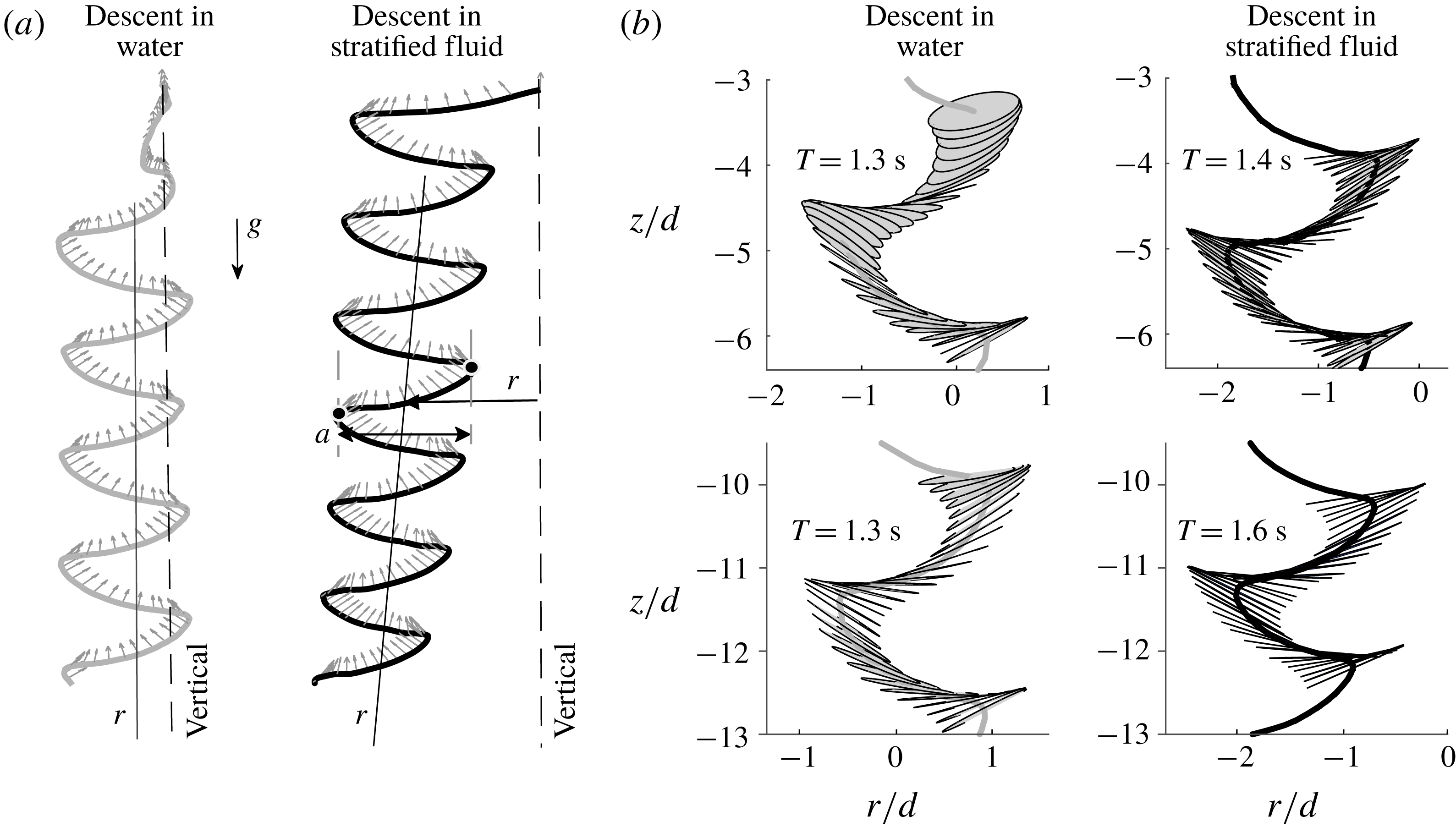
(a) Sample trajectories reconstructed from discs released with zero initial conditions in water (grey) and in stratified fluid (black), showing enhanced radial drift from the initial drop location and decrease in side-to-side fluttering amplitude. The axis of the disc (normal arrows) indicates its inclination from the vertical. The transient part of the descent in water is characterized by a large out-of-plane component. (b) Snapshots of two fluttering periods at different depths for water and stratified fluid (
 $Fr=1.26$
), showing the vertical and horizontal contraction of the trajectory and the increase of the fluttering period in the stratified case.

4 Experimental observations
We compare the descent behaviour of the disc in a homogenous fluid to that in a stratified fluid. Figure 3 shows two individual trajectories for pure water and stratified fluid of
 $Fr=1.26$
, respectively. In figure 3(b), we compare two segments of the descent trajectories taken shortly after release (top row in figure 3
b) and at later depth (bottom row in figure 3
b). Each segment includes a full oscillation cycle of the fluttering disc. In pure water, the amplitude and period of oscillation is independent of depth; the oscillation period is
 $T=1.3$
s and the descent speed is about
 $3.2\,d$
per flutter cycle or
 $2.5\,d~\text{s}^{-1}$
. In the stratified environment, the speed of the disc decreases with depth. Initially, the disc descends about
 $2.5\,d$
in
 $T\simeq 1.4$
s, and near the bottom, it takes
 $T\simeq 1.6$
s to cover the same distance. That is, the vertical speed decreases from
 $1.8\,d~\text{s}^{-1}$
to
 $1.6\,d~\text{s}^{-1}$
.
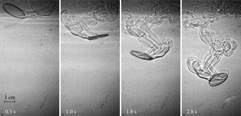
The fluid movement induced by the descending disc in the stratified environment is visualized using a direct shadowgraph technique: a small bright light source casts shadows on the screen as light is refracted by the perturbed fluid (see Merzkirch Reference Merzkirch1987; Settles Reference Settles2012). Figure 4 shows snapshots of the flow for
 $Fr=1.31$
. Initially, the vortex structure is similar to that shown by Zhong et al. (Reference Zhong, Lee, Su, Chen, Zhou and Wu2013) for planar fluttering in water, with the wake consisting of primary vortices, secondary vortices and counter-rotating vortex pairs. At later times, the secondary vortices disappears and the wake resembles those of hula-hooping or spiralling descents Lee et al. (Reference Lee, Su, Zhong, Chen, Zhou and Wu2013).
Shadowgraph flow visualization at various times of a free-falling fluttering disc in stratified fluid (
 $Fr=1.31$
;
 $N=1.63~\text{rad}~\text{s}^{-1}$
).

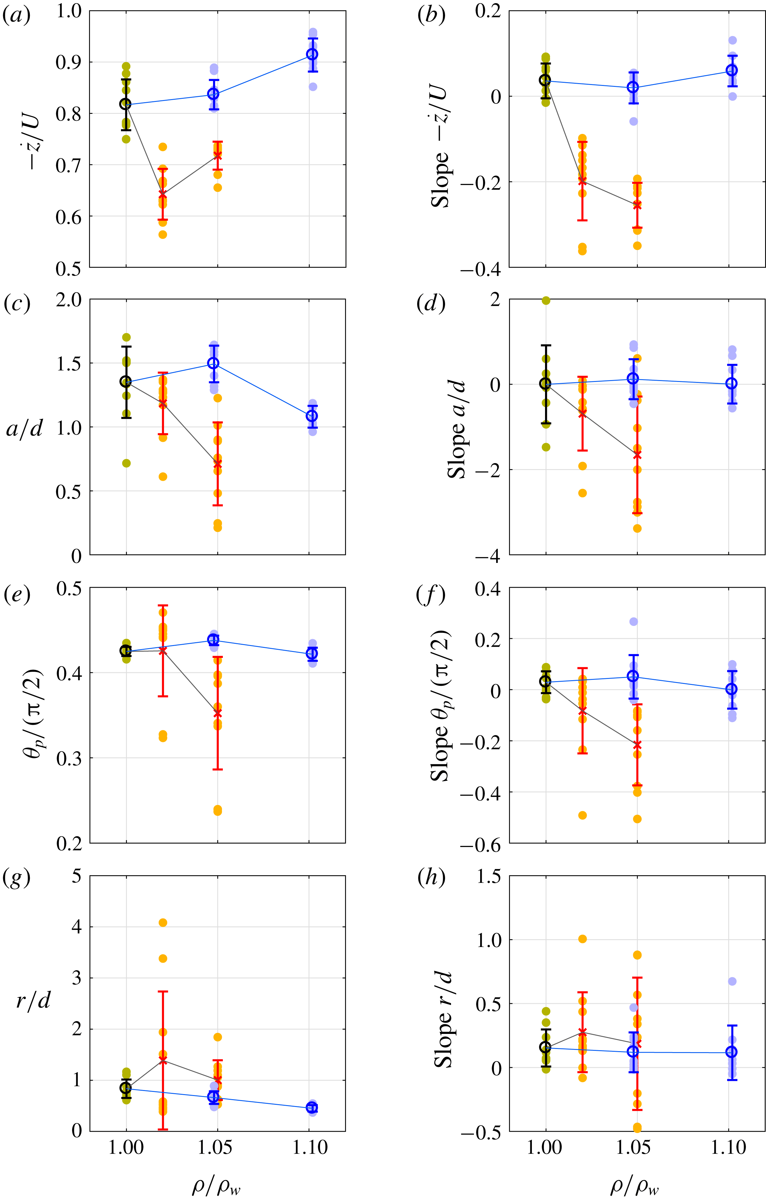
(a,c,e,g) Average descent speed
 ${\dot{z}}$
, fluttering peak-to-peak amplitude
 $a$
, peak inclination
 $\unicode[STIX]{x1D703}_{p}$
and radial range
 $r$
, averaged over the entire duration of the descent motion, for various fluid densities and fluid types: pure water
 $\unicode[STIX]{x1D70C}/\unicode[STIX]{x1D70C}_{w}=1$
(green), saltwater (blue) of uniform density for two density values
 $\unicode[STIX]{x1D70C}/\unicode[STIX]{x1D70C}_{w}=1.048$
and
 $1.102$
and stratified saltwater fluid (orange) at two levels of stratification
 $Fr=2.34$
and
 $1.26$
. (b,d,f,h) The linear slope with respect to depth of each variable based on the best linear data fit. Mean fluid density values are used for stratified fluid when computing
 $\unicode[STIX]{x1D70C}/\unicode[STIX]{x1D70C}_{w}$
, where
 $\unicode[STIX]{x1D70C}_{w}$
is the density of water. Here
 $U$
is the terminal speed, accounting for buoyancy. The
 $1-\unicode[STIX]{x1D70E}$
uncertainty bars are included for each data set. Stratification induces longer descent time, smaller fluttering amplitude, smaller peak inclination and appear to have larger radial dispersions.

To systematically quantify the effect of stratification on the descent behaviour, we consider the three fluid environments described in § 3 and listed in table 1: pure water
 $\unicode[STIX]{x1D70C}_{w}$
, saltwater of uniform density for two density values
 $\unicode[STIX]{x1D70C}/\unicode[STIX]{x1D70C}_{w}=1.048$
and
 $1.102$
and stratified saltwater fluid at two levels of stratification
 $Fr=2.34$
and
 $1.26$
. In each environment, we repeatedly drop the disc ten times and reconstruct the descent trajectories for each drop. For each reconstructed trajectory, we calculate the following quantities: the speed of descent
 ${\dot{z}}$
, the peak-to-peak amplitude
 $a$
of each flutter oscillation (see figure 3
a) and the inclination angle
 $\unicode[STIX]{x1D703}_{p}$
of the disc at ‘peak’ positions of each oscillation cycle where the disc reverses direction. We also examine the effect of stratification on the horizontal dispersion of the disc, which we define as the radial coordinate
 $r$
away from the drop location of the disc (see figure 3
a).
We normalize
 $z$
by the height
 $h$
,
 $a$
and
 $r$
by the disc diameter
 $d$
,
 $\unicode[STIX]{x1D703}_{p}$
by
 $\unicode[STIX]{x03C0}/2$
and
 ${\dot{z}}$
by the terminal speed
 $U$
. Although the descent regime is typically characterized by the disc diameter
 $d$
, because of the linear density stratified fluid, the tank height
 $h$
is also an important length scale. In particular, the value of
 $h$
provides a qualitative estimate of the density value encountered by the disc. We therefore use both
 $d$
and
 $h$
as typical length scales. To avoid confusion, we clearly label the non-dimensional quantities in the text and all figures. Figure 5(a,c,e,g) depicts the normalized values
 ${\dot{z}}/U$
,
 $a/d$
,
 $2\unicode[STIX]{x1D703}_{p}/\unicode[STIX]{x03C0}$
,
 $r/d$
averaged over each descent trajectory, as functions of the average density ratio
 $\unicode[STIX]{x1D70C}/\unicode[STIX]{x1D70C}_{w}$
of the fluid. Values corresponding to each descent trajectory are represented by a filled circle. For each fluid medium, the average (open circle) and standard deviation (vertical bar) over all ten descent trajectories are superimposed. Results are depicted in green for pure water, blue for homogeneous saltwater and red for the stratified fluids. To emphasize that
 ${\dot{z}}/U$
,
 $a/d$
,
 $2\unicode[STIX]{x1D703}_{p}/\unicode[STIX]{x03C0}$
and
 $r/d$
vary with depth
 $-z/h$
, we calculate the slope with respect to depth associated with the best linear fit for each trajectory. The slope of each trajectory, as well as the average and standard deviation over all ten trajectories per fluid medium, are depicted in figure 5(b,d,f,h).
We make three observations based on figure 5(a–f).
(i) Descent speed: the vertical speed of descent is slower in stratified fluids compared with constant-density fluids. The speed
 ${\dot{z}}$
normalized by the terminal speed
$U$
decreases at
$\unicode[STIX]{x1D70C}/\unicode[STIX]{x1D70C}_{w}=1.02$
, then increases at
$\unicode[STIX]{x1D70C}/\unicode[STIX]{x1D70C}_{w}=1.05$
. This is an artefact of the normalization with
$U$
, indicating that the descent speed for the weaker stratification is slower than the theoretical terminal speed. The speed
${\dot{z}}$
decreases monotonically. The negative slope of
${\dot{z}}/U$
indicates that in stratified fluids, the disc slows down with increasing depth. In constant-density fluids, the speed is nearly constant with depth, and approaches the terminal speed with increasing fluid density (figure 5
a,b).
(ii) Fluttering amplitude: in constant-density fluid, the amplitude of oscillations does not change with depth. In stratified fluids, the fluttering amplitude decreases with increasing depth and increasing stratification strength (figure 5 c,d).
(iii) Inclination angle: the peak inclination
$\unicode[STIX]{x1D703}_{p}$
of the disc decreases in stratified fluids. The negative slope of
$\unicode[STIX]{x1D703}_{p}$
indicates that in stratified fluids, the peak inclination continues to decrease with increasing depth (figure 5
e,f).(iv) Radial dispersion: the radial dispersion away from the drop location seems to increase in stratified fluids. We explore this observation further in § 7.


The slowing down of the vertical motion for the stratified fluid case is consistent with intuition. As the density increases with depth, the buoyancy-corrected weight decreases and drag increases, thus decelerating the descending disc and increasing the descent time. However, the decrease of both the oscillation amplitude and peak inclination in stratified fluids, as well as the change of these quantities with depth, are less intuitive. In § 5, we explore the physical mechanisms underlying these observations, and in § 6, we develop a quasi-steady model that reproduces similar results by incorporating the mechanisms proposed in § 5. To conclude this section, we note that the radial dispersion seems to increase in stratified fluids for discs released horizontally from rest. However, these results are not conclusive given that the sample size is small and the variance between trials is large. We return to this issue in § 8.
5 Physical mechanisms
In this section, we discuss the physical mechanisms causing the vertical speed, fluttering amplitude and inclination angle to decrease with depth in stratified fluids. We focus our analysis on a subset of the experimental data reported in figure 5: ten descents in water and ten descents in stratified fluid at
 $Fr=1.26$
. We expect the underlying mechanisms to be applicable to all the other cases.
5.1 Apparent drag enhancement
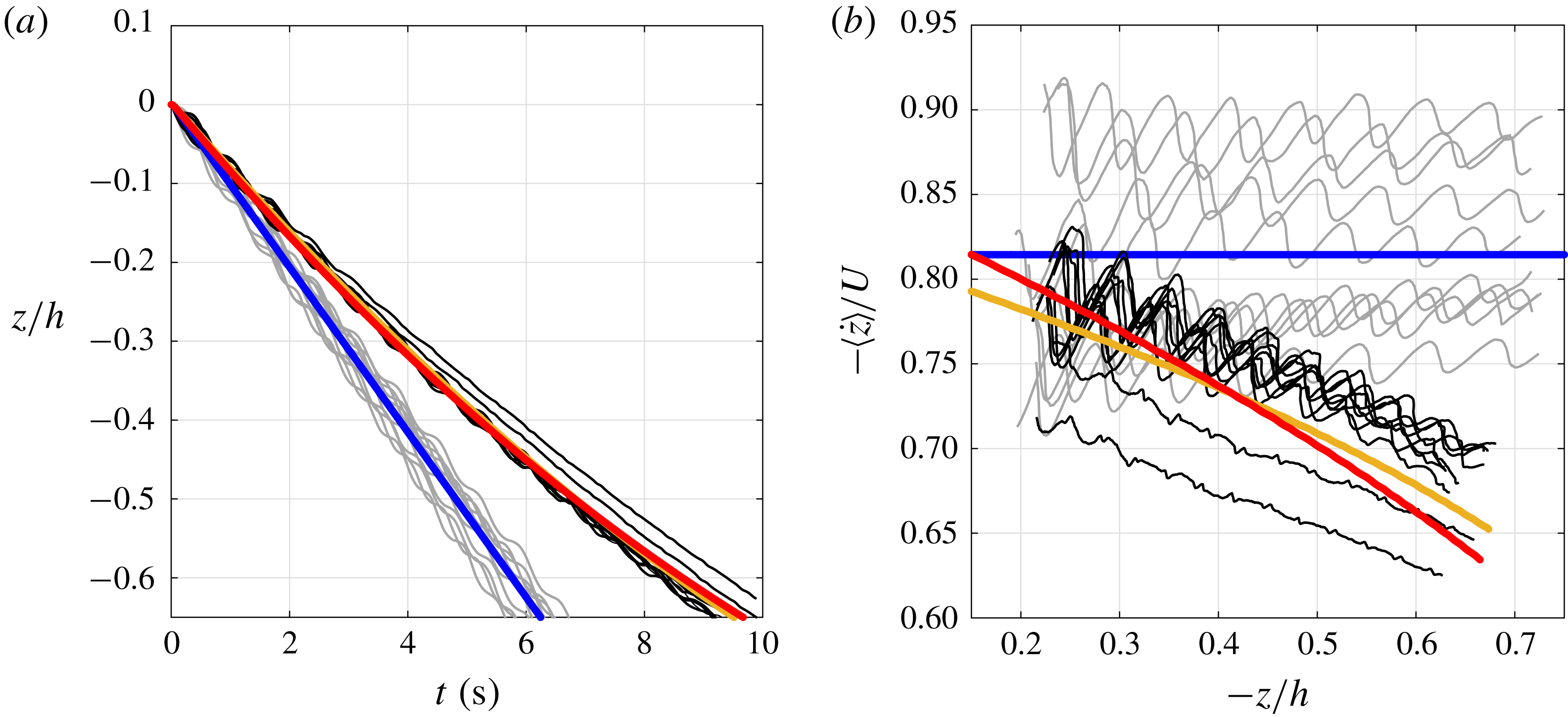
Figure 6(a) shows the vertical position
 $z$
of the centre of the disc as a function of time for the ten descents in water and ten descents in stratified fluid at
 $Fr=1.26$
. Clearly, the descent time is higher in the stratified case: 10 s in stratified fluid as compared with 6.5 s in pure water. Furthermore, the slope of
 $\text{d}z/\text{d}t$
is not linear in stratified fluid, indicating a deceleration in speed as the disc descends. Blanchette & Bush (Reference Blanchette and Bush2005) noted similar descent profiles for sediments in stratified fluids. Figure 6(b) depicts the time-averaged descent velocity as a function of depth
 $-z/h$
(not to be confused with the average over the whole descent in figure 5
a). It clearly shows the vertical deceleration in stratified fluids. In pure water, the average velocity is almost constant,
 $\langle {\dot{z}}\rangle /U=-0.816\pm 0.05$
with a small negative slope (linear fit of
 $-0.045$
) with respect to depth. For
 $Fr=1.26$
, the average descent speed approaches
 $\langle {\dot{z}}\rangle /U=-0.715\pm 0.03$
, with a non-zero slope (linear fit of 0.175) indicating deceleration with respect to depth.
The descents in water follow side-to-side fluttering whereas in stratified fluid we observed two types of fluttering: side-to-side fluttering and gyroscopic (hula-hoop) fluttering. In figure 6, the hula-loop motion occurred in two of the ten stratified cases. For these descents, the disc does not heave and its inclination is fairly constant, producing a less-sinuous vertical profile, as seen in figure 6. The near-constant inclination of these two trajectories is evident in figure 7(a).
(a) Depth as a function of time, and (b) time-averaged descent velocity as a function of depth for descents in water (grey) and
 $Fr=1.26$
stratified fluid (black), where
 $h$
is the height of the tank and
 $U$
is the terminal speed (see table 1). All descents in water follow side-to-side fluttering behaviour, while the descents in the stratified fluid exhibit side-to-side and gyroscopic fluttering (the top two trajectories in (a) and bottom two trajectories in (b)). Integrated states from (5.1) are overlaid in bold lines. Here
 $C_{D}=1.44$
(blue) for the water descent with root mean square error
 $\text{RMSE}=0.002z/h$
,
 $C_{D}=1.97$
(red) with
 $\text{RMSE}=0.004z/h$
and
 $C_{D}=0.75~z/h+2.18$
(orange) with
 $\text{RMSE}=0.001z/h$
for the stratified fluid descents. The values for
 $C_{D}$
were found by performing a least-squares fit on the respective experimental
 $z$
data to an accuracy of 0.001.

The vertical descent motion in figure 6 follows closely the dynamics of a particle falling under the influence of gravity and subject to buoyancy and drag forces:
 $$\begin{eqnarray}\ddot{z}=-g+\frac{1}{m}\unicode[STIX]{x1D70C}(z){\mathcal{V}}g+\frac{1}{2m}\unicode[STIX]{x1D70C}(z)|{\dot{z}}|^{2}C_{D}S.\end{eqnarray}$$
Here,
 ${\mathcal{V}}=Se$
is the volume of the disc,
 $S=\unicode[STIX]{x03C0}d^{2}/4$
its area and
 $m=\unicode[STIX]{x1D70C}_{disc}{\mathcal{V}}$
its mass. We solve (5.1) numerically and superimpose the solution onto figure 6 using estimated values of the drag coefficient
 $C_{D}$
that best fitted experimental
 $z(t)$
averaged over all ten trajectories. The values for
 $C_{D}$
were estimated to the nearest 0.001. In pure water, we obtain
 $C_{D}=1.44$
(solid blue lines in figure 6), with root mean square error
 $\text{RMSE}=0.002z/h$
.
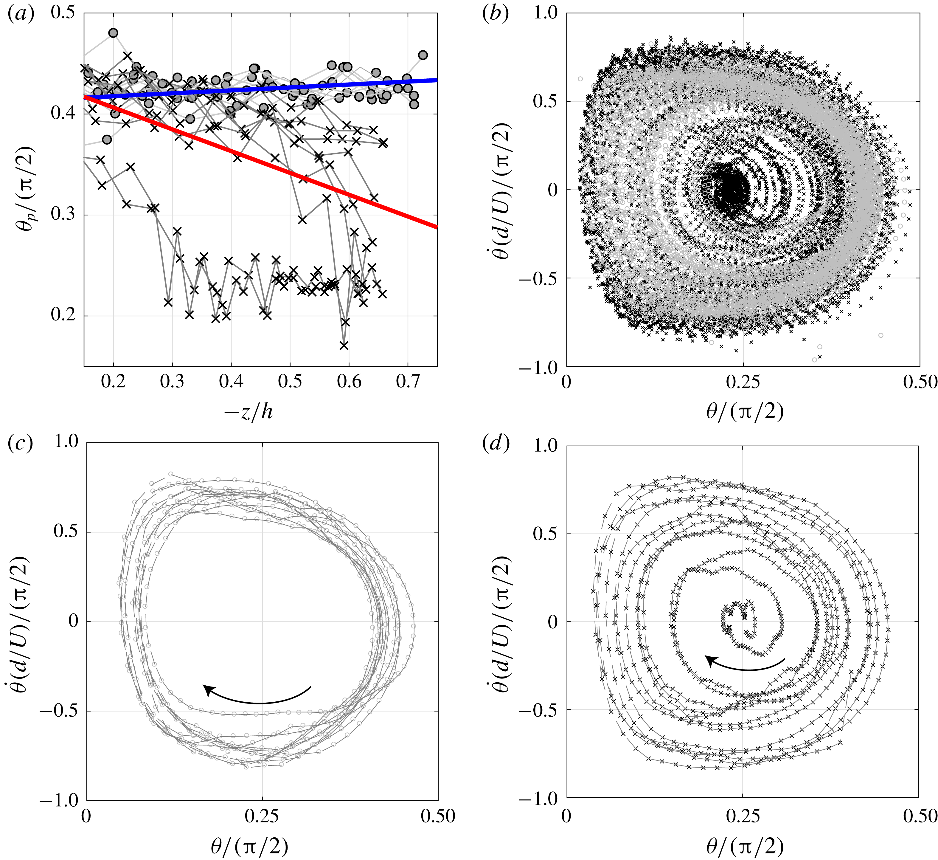
(a) Peak inclination of the disc as a function of depth
 $-z/h$
. Descents in water are in grey and descents in a stratified fluid with
 $Fr=1.26$
are in black. Linear fits of individual descents are computed and the average of the fit are overlaid for water (bold blue line) and stratified fluid (bold red line). The linear slope for descents in water is near zero while descents in stratified fluid have a negative slope. (b) Phase plot of
 $\unicode[STIX]{x1D703}$
–
 $\dot{\unicode[STIX]{x1D703}}$
for descents in water (○) and stratified fluid (
 $\times$
). A sample descent trajectory plotted in the
 $\unicode[STIX]{x1D703}$
–
 $\dot{\unicode[STIX]{x1D703}}$
plane (c) in water and (d) in the stratified fluid.

Since the descent motions in the stratified fluid exhibit both side-to-side (planar) and gyroscopic (non-planar) fluttering, an estimate of the drag coefficient
 $C_{D}$
for each descent type leads to
 $C_{D}=1.92$
for side-to-side fluttering (based on eight trajectories) and
 $C_{D}=2.32$
for gyroscopic fluttering (based on two trajectories). These estimates indicate that the drag coefficient increases in the stratified fluid in comparison with pure water. They also seem to indicate that gyroscopic motions are characterized by larger drag coefficient. However, a detailed comparison of the two types of fluttering, side-to-side versus gyroscopic, would require additional data, especially in light of the variability in the transient dynamics due to the small uncertainty in the initial conditions. Here, we make no further distinction between the two types of fluttering behaviours because we are mostly interested in highlighting the effect of stratification on the descent dynamics in comparison with pure water. To this end, we group all trajectories in the stratified fluid together. We consider two models of the drag coefficient: a constant drag coefficient (best fit is shown in red in figure 6) and a drag coefficient that varies linearly with depth
 $z$
(best fit is shown in orange). We found that for the constant coefficient model,
 $C_{D}=1.97$
matches closely the experimental data (
 $\text{RMSE}=0.004z/h$
). For the linearly varying drag coefficient, we found
 $C_{D}=0.75~z/h+2.18$
(
 $\text{RMSE}=0.001z/h$
); that is to say, the estimated drag coefficient decreases linearly with increasing depth
 $(-z/h)$
. The non-constant
 $C_{D}(z)$
is slightly better at estimating the stratified descents (
 $\text{RMSE}=0.001z/h$
versus
 $0.004z/h$
), as shown in figure 6. An advantage of the linearly varying drag coefficient is that it allows us to use (5.1) to predict the motion beyond the experimental data, whereas constant
 $C_{D}$
may only be valid for the available data. We emphasize that (5.1) ignores the horizontal and orientational motion of the disc and lumps all the dynamics into the drag coefficients. We present a more detailed model that takes into account these effects in § 6.
The constant drag coefficient in stratified fluid is noticeably larger than that of water, about 40 % larger (ratio:
 $1.97/1.44=1.37$
). Enhanced drag was observed by Torres et al. (Reference Torres, Hanazaki, Ochoa, Castillo and Van Woert2000) and Yick et al. (Reference Yick, Torres, Peacock and Stocker2009) for the vertical motion of spheres in stratified fluid, where they found correlations between
 $C_{D}$
and the Froude number
 $Fr$
. This phenomenon was investigated further by Doostmohammadi et al. (Reference Doostmohammadi, Dabiri and Ardekani2014). The increase in drag coefficient in stratified fluid (or, more specifically, its linear dependence on depth) has a major implication on the modelling and prediction of the descent motion in stratified fluid.
5.2 Buoyancy-driven restoring torque
To examine the effect of fluid stratification on the orientation dynamics of the disc, we plot in figure 7(a) the peak inclination angle
 $\unicode[STIX]{x1D703}_{p}$
as a function of depth
 $-z/h$
. The peak inclination is measured at the instants when the oscillatory motion of the disc reverses direction. Clearly, there is a notable decrease in peak inclination in the stratified fluid. The average peak inclination for the descents in water and stratified fluid are
 $\unicode[STIX]{x1D703}_{p}=0.667$
and
 $0.561$
rad, respectively. A linear fit of the respective data sets leads to
 $\unicode[STIX]{x1D703}_{p}=-0.046~z/h+0.65$
rad for the descents in pure water and
 $\unicode[STIX]{x1D703}_{p}=0.339~z/h+0.71$
rad in stratified fluid. In other words, the peak inclination remains fairly constant for the descents in pure water and decreases with depth
 $-z/h$
for the descents in stratified fluid.
In figure 7(b), we map the descent data for all ten trials in pure water and ten trials in stratified fluid onto the (
 $\unicode[STIX]{x1D703}$
,
 $\dot{\unicode[STIX]{x1D703}}$
) phase plane. For the descents in water (○), the motion is almost periodic and centred at
 $(\unicode[STIX]{x1D703},\dot{\unicode[STIX]{x1D703}})\approx (\unicode[STIX]{x03C0}/8,0)$
; this behaviour can be seen more clearly when examining a single descent trajectory as done in figure 7(c). For the descent in stratified fluid (
 $\times$
), the motion spirals inwards approaching
 $(\unicode[STIX]{x1D703},\dot{\unicode[STIX]{x1D703}})\approx (\unicode[STIX]{x03C0}/8,0)$
, as seen more clearly in the single descent trajectory shown in Figure 7(d). At
 $(\unicode[STIX]{x1D703},\dot{\unicode[STIX]{x1D703}})\approx (\unicode[STIX]{x03C0}/8,0)$
, the disc descends at a fixed inclination angle following either (i) the hula-hoop motion, where the disc’s trajectory is helical (Auguste et al.
Reference Auguste, Magnaudet and Fabre2013), or (ii) a steady straight-line descent at constant orientation.
Taken together, the results in figure 7 suggest the existence of a restoring torque in stratified fluid that dampens the orientation dynamics of the disc as it descends through the fluid. We postulate that this restoring torque is induced by the offset in the centre of gravity and the centre of buoyancy. When the inclination angle is non-zero, the side of the disc closer to the bottom of the tank will experience higher buoyancy force due to the fluid’s higher density, causing a torque in the direction which minimizes the inclination angle.
We derive an expression for the stratification-induced torque
 $T_{S}$
for a disc undergoing planar oscillations. Let the geometric centre of the disc be at height
 $z$
. The density
 $\unicode[STIX]{x1D70C}$
at a radial distance
 $\unicode[STIX]{x1D709}$
measured along the disc from its centre is given by
 $\unicode[STIX]{x1D70C}=\unicode[STIX]{x1D70C}(z)+(\text{d}\unicode[STIX]{x1D70C}/\text{d}z)\unicode[STIX]{x1D709}\sin \unicode[STIX]{x1D703}=\unicode[STIX]{x1D70C}(z)-|\unicode[STIX]{x1D6FE}|\unicode[STIX]{x1D709}\sin \unicode[STIX]{x1D703}$
. The offset distance
 $\ell$
between the geometric centre of the disc and the centre of buoyancy in stratified fluid is given by
 $$\begin{eqnarray}\ell =\frac{\displaystyle \int _{{\mathcal{V}}}(\unicode[STIX]{x1D70C}(z)-|\unicode[STIX]{x1D6FE}|\unicode[STIX]{x1D709}\sin \unicode[STIX]{x1D703})\unicode[STIX]{x1D709}\,\text{d}{\mathcal{V}}}{\unicode[STIX]{x1D70C}(z){\mathcal{V}}}.\end{eqnarray}$$
Here,
 $\text{d}{\mathcal{V}}=2\unicode[STIX]{x03C0}e\unicode[STIX]{x1D709}\,\text{d}\unicode[STIX]{x1D709}$
and
 ${\mathcal{V}}=\unicode[STIX]{x03C0}ed^{2}/8$
. Integrating over the disc’s volume
 ${\mathcal{V}}$
, we obtain
 $$\begin{eqnarray}\ell =-\frac{|\unicode[STIX]{x1D6FE}|d^{2}}{16\unicode[STIX]{x1D70C}(z)}\sin (\unicode[STIX]{x1D703}).\end{eqnarray}$$
The torque induced by this offset is given by
 $T_{S}=\unicode[STIX]{x1D70C}(z){\mathcal{V}}g\ell \cos \unicode[STIX]{x1D703}$
. Substituting (5.3) and using the definition of the Brunt–Väisälä frequency
 $N=(-\unicode[STIX]{x1D6FE}g/\unicode[STIX]{x1D70C}(z))^{1/2}$
, one obtains
 $$\begin{eqnarray}T_{S}=-{\displaystyle \frac{J}{2}}{\displaystyle \frac{\unicode[STIX]{x1D70C}(z)}{\unicode[STIX]{x1D70C}_{disc}}}N^{2}\sin (2\unicode[STIX]{x1D703}),\end{eqnarray}$$
where
 $J=\unicode[STIX]{x1D70C}_{disc}{\mathcal{V}}d^{2}/16$
is the moment of inertia of the disc about its diameter. For heavy discs with
 $\unicode[STIX]{x1D70C}_{disc}\gg \unicode[STIX]{x1D70C}$
, this torque has no effect on the rotational motion of the disc. When the disc density is comparable with the fluid density, this torque is proportional to
 $N^{2}$
; that is, if the stratification frequency doubles, the stratification-induced torque increases fourfold. The effect of this torque on the full dynamics of the disc is discussed in detail in § 6.
5.3 Effect of stratification on horizontal motion
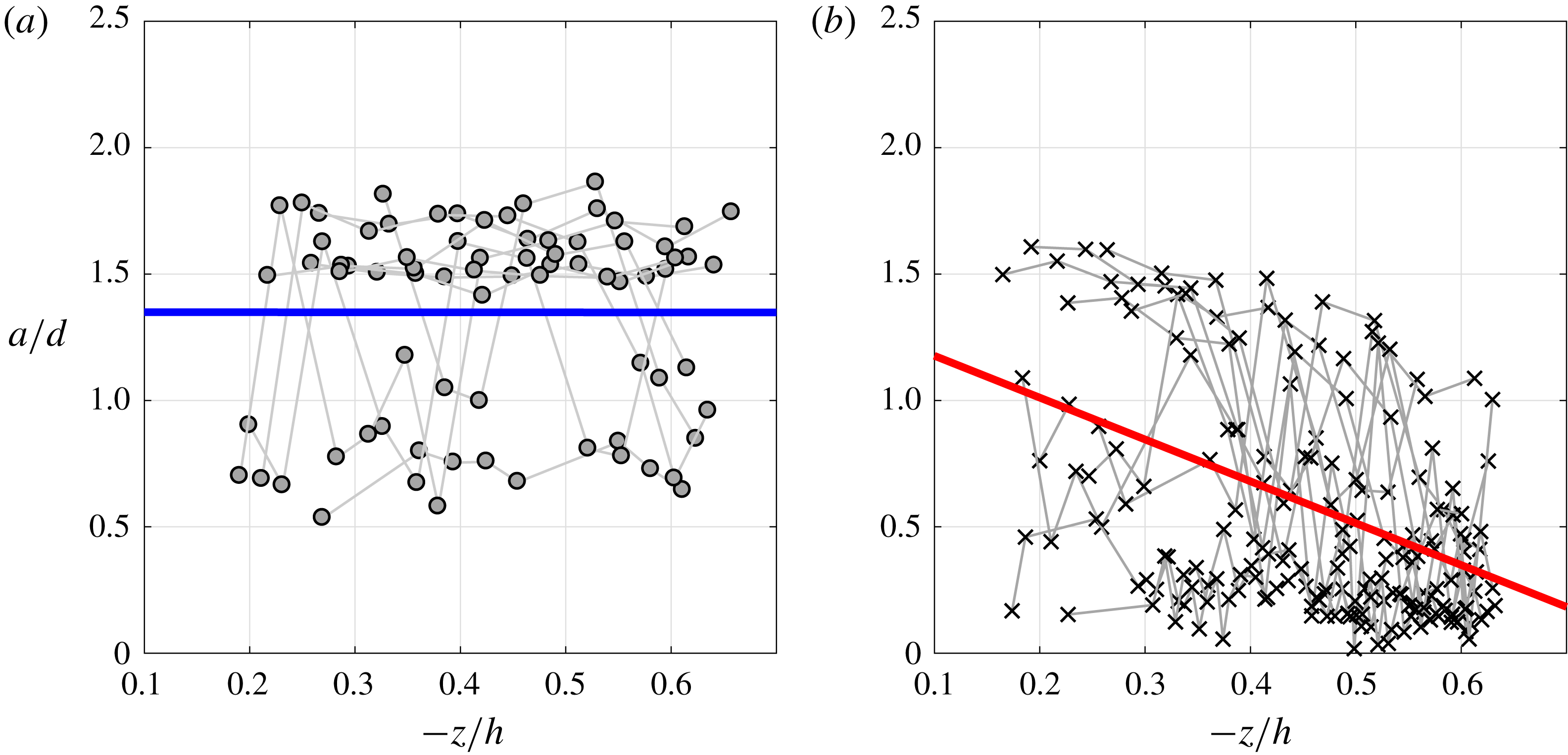
Fluttering amplitude
 $a$
versus vertical location of discs descending in (a) water and (b) stratified fluid for
 $Fr=1.26$
. Linear fits of individual descents are computed and the average of the fit is overlaid for (a) water (bold blue line) and (b) stratified fluid (bold red line).

Figure 5(c,d) shows that stratification reduces the peak-to-peak fluttering amplitude
 $a$
, with the stronger stratification leading to a twofold decrease in amplitude. In figure 8, we compare the fluttering amplitude in pure water (figure 8
a) and stratified fluid (figure 8
b) as a function of depth
 $-z/h$
. In pure water, the amplitude stays nearly constant with depth, with a linear fit of
 $a/d=-0.002~z/h+1.35$
. In stratified fluid, the fluttering amplitude decreases with depth at a rate
 $a/d=-1.656~z/h+1.34$
.
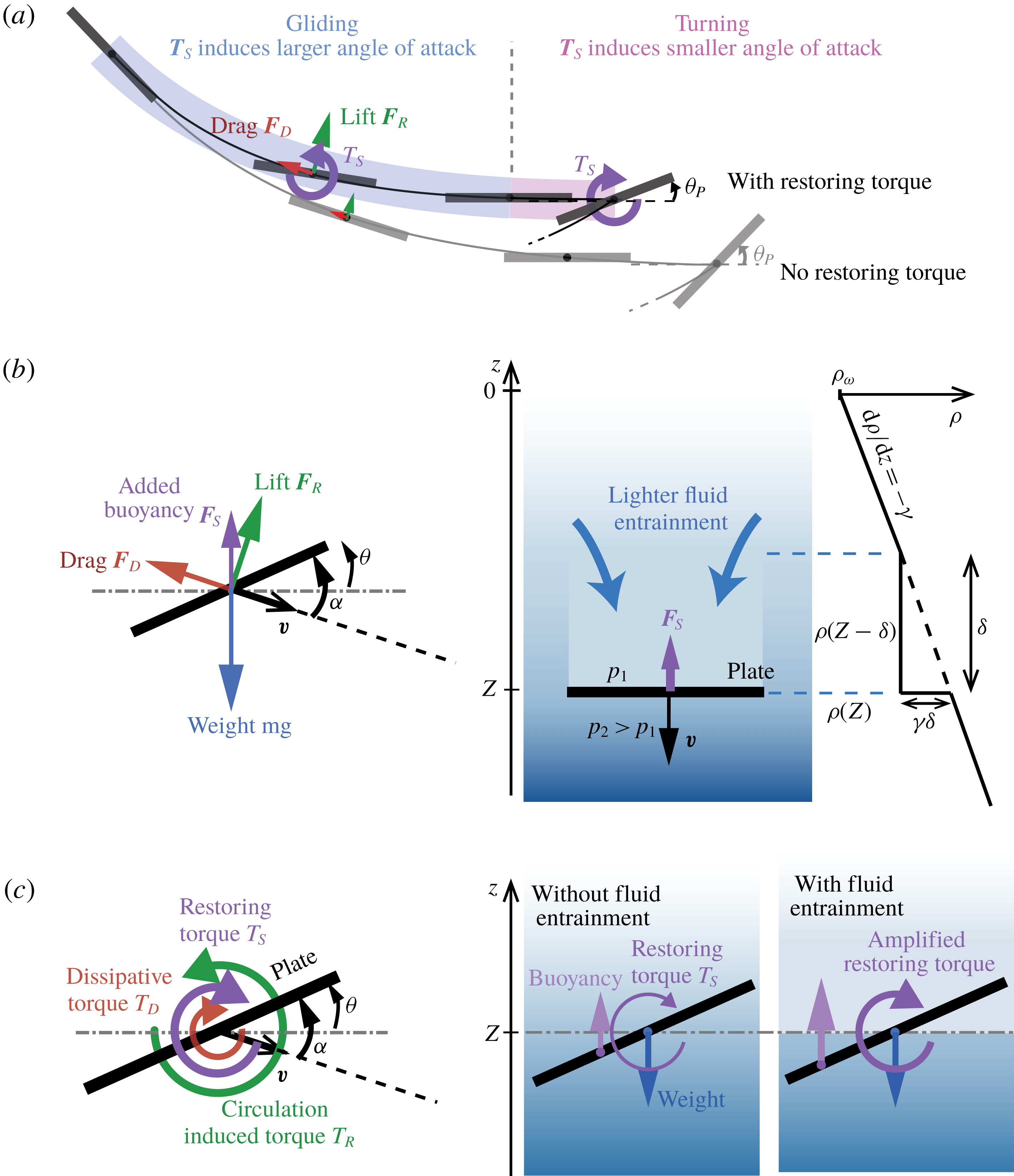
(a) Schematic representation of the expected effect of the restoring torque
 $T_{S}$
on the translational and rotational motion of a fluttering disc. During the gliding segment,
 $T_{S}$
tends to increase the angle of attack, inducing higher lift and drag forces
 $\boldsymbol{F}_{R}$
and
 $\boldsymbol{F}_{D}$
, thus shrinking and deflecting the gliding segment upwards. At the turning point,
 $T_{S}$
moderates the peak disc inclination
 $\unicode[STIX]{x1D703}_{p}$
. (b,c) Free-body diagrams of the forces and moments acting on the falling plate in the quasi-steady model in § 6. Entrainment of lighter fluid is modelled as an area of constant density in the wake of the disc; the added buoyancy force
 $\boldsymbol{F}_{S}$
is calculated from the resulting density and pressure jumps. The density jump also amplifies the restoring torque
 $T_{S}$
.

We argue that the buoyancy-induced restoring torque in (5.4) is responsible for the reduction in fluttering amplitude. As the disc starts gliding (see figure 9
a), the restoring torque causes it to pitch up, thus increasing its angle of attack. The latter is defined as the angle between the disc and its velocity vector and is denoted by
 $\unicode[STIX]{x1D6FC}$
(figure 9
b). The increase in angle of attack, in turn, increases both lift and drag. Increased lift deflects the trajectory upwards, while increased drag slows down the horizontal motion, causing the gliding segment to end sooner than in pure water. As the disc begins to turn past its horizontal orientation, the restoring torque now reduces the angle of attack, which causes the disc to drift slightly further in the turning segment for the stratified case. However, the increased drift in the turning segment is not sufficient to compensate for the decrease in the gliding segment, because the former is much shorter than the latter, resulting in an overall shortening of the fluttering amplitude in stratified fluid.
Our proposed mechanism can be used to explain the behaviour in figure 5(d), which shows that the fluttering amplitude decreases with depth, with stronger stratification inducing a steeper reduction. As depth increases, the density ratio between the disc and the fluid approaches unity. Consequently, the disc’s velocity decreases, leading to smaller hydrodynamic forces and moments, since they all depend quadratically on the velocity. In contrast, the restoring torque in (5.4) only depends on the local density ratio
 $\unicode[STIX]{x1D70C}(z)/\unicode[STIX]{x1D70C}_{disc}$
, which increases with depth. It is therefore expected that the relative effect of the restoring torque increases significantly with depth, hence leading to a reduction in fluttering amplitude as depth increases.
6 Quasi-steady model
Quasi-steady force models have been widely used in the context of falling discs and plates in homogeneous fluids; see e.g. Tanabe & Kaneko (Reference Tanabe and Kaneko1994), Pesavento & Wang (Reference Pesavento and Wang2004), Andersen et al. (Reference Andersen, Pesavento and Wang2005a ) and Hu & Wang (Reference Hu and Wang2014). Inspired by this body of literature and based on our experimental observations, we formulate a new quasi-steady model for two-dimensional descent motions in stratified fluids.
In two dimensions, we represent the disc as a thin elongated ellipse with major axis
 $d$
and minor axis
 $e$
. We introduced a orthonormal frame
 $(\boldsymbol{b}_{1},\boldsymbol{b}_{2},\boldsymbol{b}_{3})$
centred at the ellipse with
 $\boldsymbol{b}_{1}$
along the major axis and
 $\boldsymbol{b}_{2}$
along the minor axis.
We start from the balance of linear and angular momenta on the rigid disc, written in the disc-fixed frame, and we account for lift, drag and buoyancy effects (see figure 9 b,c). This includes the restoring torque and the added buoyancy force due to fluid entrainment. The equations of motion governing the motion of the disc can be written in vector form as follows:
 $$\begin{eqnarray}\left.\begin{array}{@{}c@{}}\dot{\boldsymbol{P}}=\boldsymbol{P}\times \unicode[STIX]{x1D734}+\boldsymbol{F}_{D}+\boldsymbol{F}_{R}+\boldsymbol{F}_{S}-(m-m_{b})g\boldsymbol{k},\\ \dot{\unicode[STIX]{x1D72B}}=\boldsymbol{P}\times \boldsymbol{V}+\boldsymbol{T}_{D}+\boldsymbol{T}_{R}+\boldsymbol{T}_{S}.\end{array}\right\}\end{eqnarray}$$
Here,
 $\boldsymbol{P}=(m\unicode[STIX]{x1D644}+\unicode[STIX]{x1D648}_{add})\boldsymbol{V}$
and
 $\unicode[STIX]{x1D72B}=(J+J_{add})\unicode[STIX]{x1D734}$
are the linear and angular momenta of the disc expressed in body frame. The symbol
 $\unicode[STIX]{x1D644}=\text{diag}\{1,1\}$
denotes the identity matrix. The mass and moment of inertia of the disc are
 $m=\unicode[STIX]{x03C0}\unicode[STIX]{x1D70C}_{disc}ed/4$
and
 $J=\unicode[STIX]{x03C0}\unicode[STIX]{x1D70C}_{disc}ed(e^{2}+d^{2})/64$
, respectively. The buoyancy-corrected mass is
 $m-m_{b}=\unicode[STIX]{x03C0}(\unicode[STIX]{x1D70C}_{disc}-\unicode[STIX]{x1D70C}(z))ed/4$
. The added mass for an elliptical object is
 $\unicode[STIX]{x1D648}_{add}=\unicode[STIX]{x03C0}\unicode[STIX]{x1D70C}(z)\,\text{diag}\{d^{2},e^{2}\}/4$
and the added moment of inertia is
 $J_{add}=\unicode[STIX]{x03C0}\unicode[STIX]{x1D70C}(z)(d^{2}-e^{2})^{2}/32$
. The unit vector
 $\boldsymbol{k}=\sin \unicode[STIX]{x1D703}\boldsymbol{b}_{1}+\cos \unicode[STIX]{x1D703}\boldsymbol{b}_{2}$
points vertically up in the
 $z$
-direction.
In (6.1),
 $\boldsymbol{F}_{D}$
and
 $\boldsymbol{T}_{D}$
denote the force and torque due to drag. Following Andersen et al. (Reference Andersen, Pesavento and Wang2005a
,Reference Andersen, Pesavento and Wang
b
), we model the drag force as a quadratic function of the angle of attack, which we denote by
 $\unicode[STIX]{x1D6FC}$
:
 $$\begin{eqnarray}\displaystyle \boldsymbol{F}_{D}=-{\textstyle \frac{1}{2}}e\unicode[STIX]{x1D70C}(z)(C_{D}(0)\cos ^{2}\unicode[STIX]{x1D6FC}+C_{D}(\unicode[STIX]{x03C0}/2)\sin ^{2}\unicode[STIX]{x1D6FC})|V|\boldsymbol{V}. & & \displaystyle\end{eqnarray}$$
Here,
 $C_{D}(0)$
and
 $C_{D}(\unicode[STIX]{x03C0}/2)$
are drag coefficients at
 $\unicode[STIX]{x1D6FC}=0$
and
 $\unicode[STIX]{x1D6FC}=\unicode[STIX]{x03C0}/2$
, respectively. The dissipative torque is modelled as
 $$\begin{eqnarray}\displaystyle \boldsymbol{T}_{D}=-{\textstyle \frac{1}{16}}\unicode[STIX]{x1D707}\unicode[STIX]{x03C0}\unicode[STIX]{x1D70C}d^{4}|\dot{\unicode[STIX]{x1D703}}|\dot{\unicode[STIX]{x1D703}}. & & \displaystyle\end{eqnarray}$$
where
 $\unicode[STIX]{x1D707}$
is a dimensionless constant.
Flow circulation around the falling disc induces a translation force
 $\boldsymbol{F}_{R}=\unicode[STIX]{x1D70C}\unicode[STIX]{x1D6E4}\,\boldsymbol{b}_{3}\times \boldsymbol{V}$
, where
 $\unicode[STIX]{x1D6E4}$
is the circulation around the disc and
 $\boldsymbol{b}_{3}$
is a unit vector perpendicular to the plane of motion. The circulation
 $\unicode[STIX]{x1D6E4}$
depends on both the translational speed and the angular velocity of the disc,
 $$\begin{eqnarray}\displaystyle \unicode[STIX]{x1D6E4}=-{\textstyle \frac{1}{2}}C_{T}e|V|\sin 2\unicode[STIX]{x1D6FC}+C_{R}e^{2}\dot{\unicode[STIX]{x1D703}}, & & \displaystyle\end{eqnarray}$$
where
 $C_{T}$
is the dimensionless translational lift coefficient and
 $C_{R}$
is the dimensionless rotational lift coefficient. We assume that the circulation-induced torque
 $\boldsymbol{T}_{R}$
is zero.
Finally,
 $\boldsymbol{F}_{S}$
and
 $\boldsymbol{T}_{S}$
are the force and torque due to density stratification. We argued in § 5.2 that stratification induces a buoyancy-driven restoring torque due to the offset between the centre of mass and the centre of buoyancy, leading to
 $\boldsymbol{T}_{S}=T_{S}\boldsymbol{b}_{3}$
, where
 $T_{S}$
is given in (5.4). Stratification also induces an additional buoyancy force
 $\boldsymbol{F}_{S}$
that arises from the fact that the disc entrains lighter fluid into regions of higher-density fluid as it falls. This phenomenon was acknowledged by previous work on axisymmetric objects moving through stratified fluids (see Torres et al.
Reference Torres, Hanazaki, Ochoa, Castillo and Van Woert2000; Yick et al.
Reference Yick, Torres, Peacock and Stocker2009; Doostmohammadi et al.
Reference Doostmohammadi, Dabiri and Ardekani2014) without quantifying this effect. Here, we model the entrainment as a volume of fluid of vertical extent
 $\unicode[STIX]{x1D6FF}$
and of constant density
 $\unicode[STIX]{x1D70C}(Z-\unicode[STIX]{x1D6FF})$
above the disc, where
 $Z$
is the current position of the disc (see figure 9
b). We assume that the fluid below the disc is unperturbed, leading to a density jump at height
 $Z$
. The pressure jump at the disc is computed by integrating the density profile
 $\unicode[STIX]{x1D70C}(z)$
over the area below and above the disc, resulting in
 $p_{2}-p_{1}=-(1/2)g\unicode[STIX]{x1D6FF}^{2}\unicode[STIX]{x1D6FE}$
(right panel of figure 9
b). The added buoyancy force due to fluid entrainment is therefore equal to, in the plate’s rotating reference frame,
 $$\begin{eqnarray}\boldsymbol{F}_{S}=-{\textstyle \frac{1}{2}}g\unicode[STIX]{x1D6FF}^{2}\unicode[STIX]{x1D6FE}d\cos (\unicode[STIX]{x1D703})(\sin \unicode[STIX]{x1D703}\boldsymbol{b}_{1}+\cos \unicode[STIX]{x1D703}\boldsymbol{b}_{2}).\end{eqnarray}$$
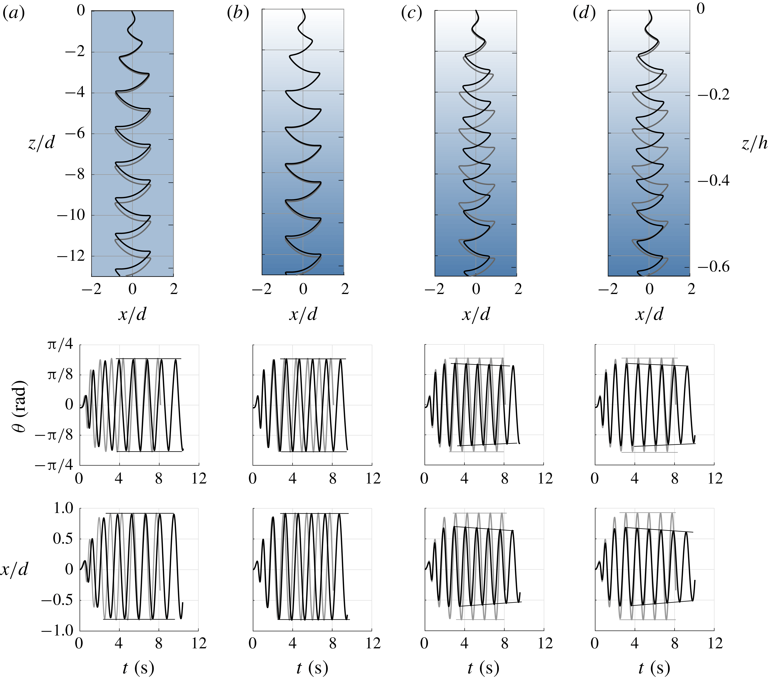
Quasi-steady model: comparison between descent motion in pure water (grey lines) and higher density or stratified fluid (black lines). The top row shows the descent trajectories in the
 $(x,z)$
plane, the middle row the inclination angle
 $\unicode[STIX]{x1D703}$
versus time, and the bottom row the fluttering motion in the
 $x$
-direction versus time. (a) Pure water versus higher density fluid (
 $\unicode[STIX]{x1D70C}/\unicode[STIX]{x1D70C}_{w}=1.05$
), (b) pure water versus stratified fluid (
 $\unicode[STIX]{x1D6FE}=-290~\text{kg}~\text{m}^{-4}$
) with
 $T_{S}=0$
and
 $F_{S}=0$
, (c) pure water versus stratified fluid with
 $F_{S}=0$
and (d) pure water versus stratified fluid.

We solve the system of equations (6.1) numerically. In all simulations, we set
 $d/e=0.0787$
,
 $I=0.0023$
,
 $C_{T}=2.0$
,
 $C_{R}=0.6$
,
 $C_{D}(0)=0.15$
,
 $C_{D}(\unicode[STIX]{x03C0}/2)=2.0$
and
 $\unicode[STIX]{x1D707}=0.33$
. In figure 10(a), we compare the descent trajectory in pure water (grey lines) to that in saltwater (black lines) at uniform density
 $\unicode[STIX]{x1D70C}=1.05\unicode[STIX]{x1D70C}_{w}$
. The two trajectories exhibit the same peak inclination and fluttering amplitude and only differ in the descent time. In figure 10(b), we compare the trajectories in pure water and stratified fluid (
 $\unicode[STIX]{x1D6FE}=-290~\text{kg}~\text{m}^{-4}$
) without taking into account the buoyancy-driven restoring torque
 $T_{S}$
and added buoyancy force
 $\boldsymbol{F}_{S}$
. Again, we see little difference between the two trajectories. This implies that changes in density in the fluid medium alone have only a small effect on the orientation and the translational motion of the descending disc. In figure 10(c), we take into account the buoyancy-driven restoring torque
 $T_{S}$
due to stratification, which results in a more prominent effect on the descent trajectory compared to pure water; namely, both the orientation angle (
 $\unicode[STIX]{x1D703}$
) and the fluttering amplitude (shown in
 $x/d$
) decrease as the disc descends, in agreement with our experimental observations. Lastly, in figure 10(d), we account for both
 $T_{S}$
and
 $\boldsymbol{F}_{S}$
and obtain similar behaviour. In sum, the numerical results based on (6.1), when accounting for the forces and moment due to stratification, exhibit increased descent time and reduced inclination angle and fluttering amplitude, consistent with our experimental observations in §§ 3 and 4.
7 Radial dispersion
We have shown, using a combination of experiments and analytical modelling, that stable vertical stratification in the fluid density affects the descent dynamics of freely falling discs. Specifically, stratification decreases the side-to-side fluttering amplitude and maximum disc inclination while increasing the descent time.
We now revisit the effect of stratification on the radial dispersion away from the disc drop location. We recall that the results presented in figure 5(g,h) indicate that the radial dispersion
 $r$
increases in stratified fluids. However, these results are not conclusive given the small sample size (ten drops in each case) and the large variability between drops due to amplification of the uncertainty in the initial conditions by the fluid–structure interactions.
The problem of a disc falling in a fluid medium is deterministic in the sense that, given a set of initial conditions, the subsequent motion of the disc follows the classic laws of mechanics (balance of linear and angular momenta). Experimentally, the electromagnetic clamp used to release the disc horizontally at zero velocity introduces a small uncertainty in the initial conditions. To quantify the variations in these initial conditions, we repeatedly dropped a heavy disc in air, as detailed in § 3. We found the standard deviation in the landing position to be less than 0.0015 of the descent height
 $h$
. This implies that the initial conditions can be described by a tight p.d.f. with small variance.
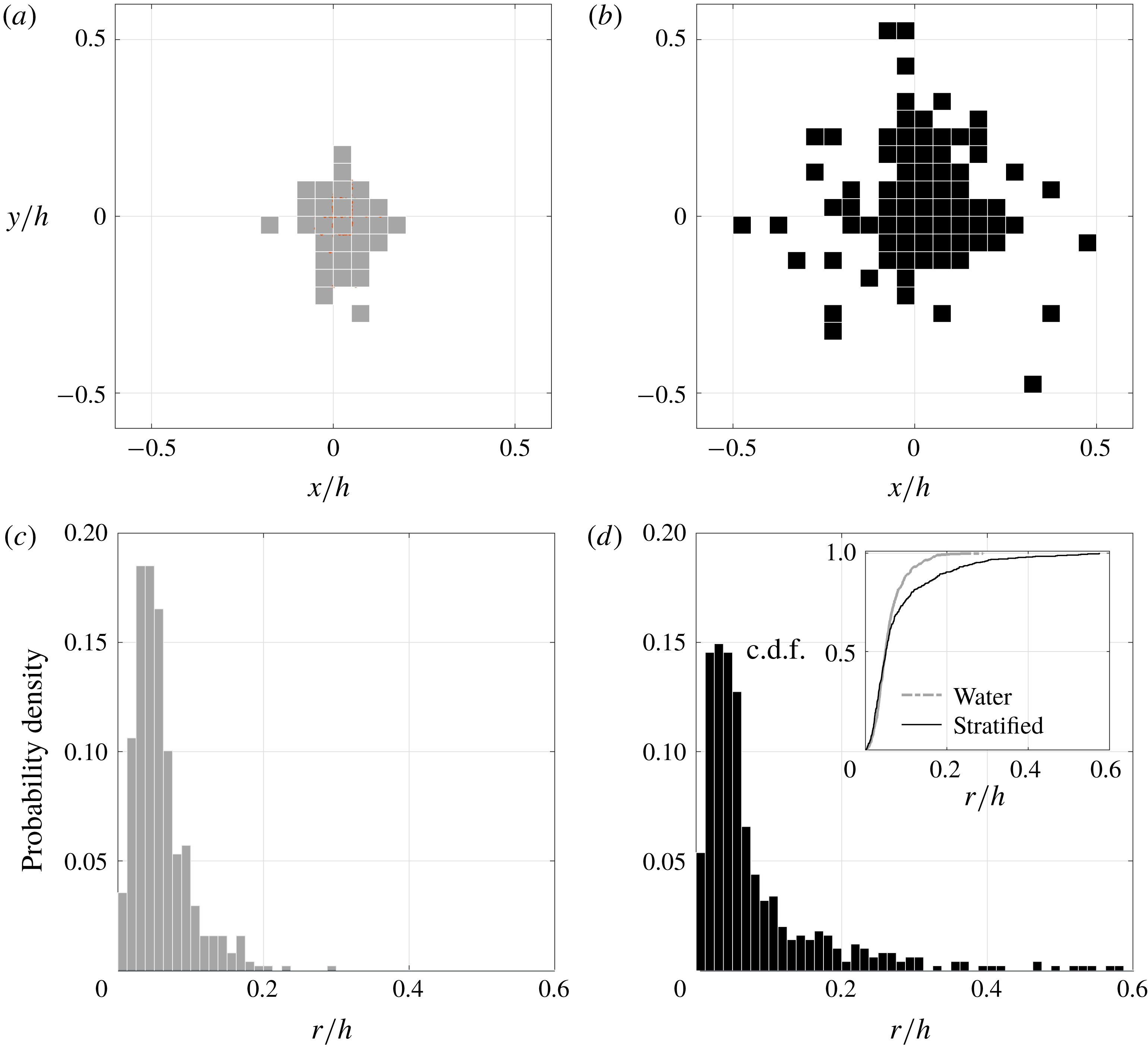
To test whether the enhanced dispersion is statistically significant, we collect the dispersion distance from a larger data set. Following Heisinger et al. (Reference Heisinger, Newton and Kanso2014), we conduct 500 drops in pure water and 500 drops in stratified fluid at
 $Fr=1.26$
. Owing to the small uncertainty in the drop mechanism, for the same fluid and disc parameters, distinct drops result in distinct falling trajectories and landing positions. We recorded the landing position of each drop and constructed the p.d.f.s of the landing sites in the
 $(x,y)$
-plane for all drops in water and in stratified fluid. The p.d.f.s are shown in figures 11(a) and 11(b), respectively. Descent in stratified fluid is characterized by a larger dispersion away from the drop location at
 $(0,0)$
, with average standard deviation approximately 1.92 times larger than in water. The corresponding radial distribution is shown in figure 11(c,d). The results in water (figure 11
c) are similar to those reported in Heisinger et al. (Reference Heisinger, Newton and Kanso2014), where they observed a dip near the origin and a tight radial distribution around the origin (standard deviation
 $\unicode[STIX]{x1D70E}<10\,\%$
of the descent height). The larger radial distribution in stratified fluid is also evident when comparing figures 11(c,d), where the variance is
 $0.002h$
for descents in water and
 $0.011h$
for descents in stratified fluid. The cumulative distribution functions for both pure water and stratified fluid are shown in the inset of figure 11(d). The two curves deviate quickly after
 $r/h>0.05$
. At
 $r/h=0.11$
, 90 % of the descents in water are accounted for. For the descents in stratified fluid, the 90 % cumulation is reached at
 $r/h=0.20$
. A summary of the distribution parameters is listed in table 2. These results provide evidence that density stratification enhances dispersion.
Landing distribution in the
 $(x,y)$
plane for 500 consecutive drops in water in (a) and (c) and in stratified fluid in (b) and (d). Cumulative distribution functions (c.d.f.s) are shown in the inset of (d). Discs are initially released from
 $(x,y)=(0,0)$
. The stratified fluid has
 $Fr=1.26$
.

The p.d.f. at landing can be interpreted as the outcome of the dynamical evolution of the tight p.d.f. of initial conditions under the nonlinear mechanics induced by the fluid–structure interactions. To illustrate this point, let the phase space of the disc be parametrized by
 $\boldsymbol{X}$
. Let the deterministic dynamics on the phase space be given by
 $\dot{\boldsymbol{X}}=\unicode[STIX]{x1D731}(\boldsymbol{X})$
, where
 $\unicode[STIX]{x1D731}=\unicode[STIX]{x1D731}_{W}$
in water and
 $\unicode[STIX]{x1D731}=\unicode[STIX]{x1D731}_{S}$
in stratified fluid;
 $\unicode[STIX]{x1D731}_{W}$
and
 $\unicode[STIX]{x1D731}_{S}$
govern both the transient and steady-state dynamics, but neither is available in closed form owing to the complex nature of the fluid–structure interactions. Further, let
 $f(\boldsymbol{X}(0))$
denote the p.d.f. of initial conditions. The time evolution of
 $f(\boldsymbol{X})$
follows the (Fokker–Planck) continuity equation
 $\unicode[STIX]{x2202}f/\unicode[STIX]{x2202}t+\unicode[STIX]{x1D735}\boldsymbol{\cdot }(f\unicode[STIX]{x1D731})=0$
, where
 $\unicode[STIX]{x1D731}$
refers to either water or stratified fluid. Experimentally, for the same
 $f(\boldsymbol{X}(0))$
(dictated by the drop mechanism), we observed that at landing
 $f(\boldsymbol{X})$
in water is less dispersed than
 $f(\boldsymbol{X})$
in stratified fluid. We associate this enhanced dispersion in the stratified fluid to the amplification of initial conditions by the deterministic ‘flow’
 $\unicode[STIX]{x1D731}$
on the phase space. Therefore, we conjecture that stratification enhances dispersion due to the inherent differences between
 $\unicode[STIX]{x1D731}_{S}(\boldsymbol{X})$
and
 $\unicode[STIX]{x1D731}_{W}(\boldsymbol{X})$
, independent of the form of
 $f(\boldsymbol{X}(0))$
.
Distribution parameters of the landing distribution for 500 free-fall fluttering discs.
 $\unicode[STIX]{x1D70E}_{1}$
and
 $\unicode[STIX]{x1D70E}_{2}$
are the standard deviations along the major and minor axes from figure 11(a,b). Here
 $r_{m}$
and
 $r_{var}$
are the mean and variance of the radial distribution normalize by the descent height
 $h$
, and c.d.f. is the cumulative distribution function as shown in figure 11(d).

This interpretation is consistent with Heisinger et al. (Reference Heisinger, Newton and Kanso2014). Heisinger and co-authors computed, for similar initial conditions, the landing p.d.f. associated with four descent regimes in pure water and showed that enhanced dispersion is usually associated with the chaotic regime (figure 2). In the chaotic regime, the fluid acts as a ‘randomization device’ that dissociates successive drops of the disc, resulting in a broadband distribution of landing sites away from the drop location and almost equal probability of landing on either side of the disc (head or tail). Stratification appears to achieve similar enhancement of radial dispersion but in the fluttering regime, where the disc never flips during its descent. In fact, stratification enhances dispersion while simultaneously reducing the fluttering amplitudes and inclination angles, making the descent trajectories closer to steady descents. These characteristics could be beneficial to many engineering and biological applications as discussed in § 8.
The exact mechanisms underlying the enhanced dispersion in the stratified fluid remain unclear. The results in §§ 5 and 6, that stratification decreases the side-to-side fluttering amplitude and maximum disc inclination while increasing the descent time, seem to suggest the opposite. However, the data set in figure 11 of the distribution of the radial position at landing clearly indicates enhanced dispersion in the stratified environment. Taken together, these results suggest that the quasi-permanent fluttering regime may not be responsible for the enhanced dispersion, and points to other mechanisms at play. Mostly, it seems that the transient behaviour and its role in amplifying the initial conditions plays an important role in the enhancement of radial dispersion, thus raising the question whether such enhancement is independent of initial conditions. The fact that the descents in the stratified fluid exhibit both side-to-side and gyroscopic fluttering while those in pure water flutter strictly side-to-side could be another reason for the enhanced dispersion. To probe the generality of the enhanced dispersion due to stratification, future experiments will be designed to explore non-horizontal initial conditions and different descent behaviours (fluttering, chaotic, tumbling) as well as to disentangle the effect of the transient regime on the overall dispersion.
Irrespective of the mechanism, enhanced dispersion in the stratified environment means that the disc drifts horizontally as it descends. Horizontal drifts were also observed by Hurlen (Reference Hurlen2006) for freely falling elliptical cylinders, both numerically and experimentally, with more subdued drifts in the latter. Biró et al. (Reference Biró, Gyure, Jánosi, Szabó and Tél2007) later noted similar drifts in the case of oscillating and levitating spheres in stratified fluid, and proposed that strong drifts are a result of a feedback of the nonlinear vortices and lee waves. In weakly stratified turbulent fluid, van Aartrijk, Clercx & Winters (Reference van Aartrijk, Clercx and Winters2008) and van Aartrijk & Clercx (Reference van Aartrijk and Clercx2010) observed enhanced horizontal dispersions for particles. Here, we postulate that the origin of such drift is due fundamentally to unsteady effects beyond what is accounted for in the quasi-steady model in § 6. The quasi-steady model, while it captures the increase in descent time and decrease in fluttering amplitude and peak inclinations of the disc, does not exhibit enhanced dispersion, even when the disc is initially given a small horizontal velocity (results not shown). The absence of radial drift in the quasi-steady model is not surprising. The model does not account for (1) unsteady force corrections, (2) effects due to the interaction of the disc and its vortices (see Andersen et al. Reference Andersen, Pesavento and Wang2005a ,Reference Andersen, Pesavento and Wang b ) or (3) three-dimensional effects. The first effect includes lift generation during acceleration from rest (Pullin & Wang Reference Pullin and Wang2004; Wang, Birch & Dickinson Reference Wang, Birch and Dickinson2004) and unsteady forces due to vortex shedding (Andersen et al. Reference Andersen, Pesavento and Wang2005a ; Lee et al. Reference Lee, Su, Zhong, Chen, Zhou and Wu2013; Zhong et al. Reference Zhong, Lee, Su, Chen, Zhou and Wu2013). Future extension of this work will focus on visualizing and quantifying the flow around the falling disc to study the unsteady vortex formation and entrainment in stratified environments and their effects on the drift dynamics.
8 Conclusions
We have experimentally investigated the motion of rigid discs falling freely in a vertically stratified fluid of saltwater solution. Starting from discs fluttering in water, we systematically varied the fluid environment to examine the effect of changes in the fluid density on the fluttering behaviour. We considered three fluid environments: pure water, constant-density saltwater (larger than that of pure water) and stratified saltwater (density varying linearly from pure water to saltwater). We found that for a disc released from rest and at a horizontal orientation (up to a small uncertainty), density stratification significantly decreases the vertical descent speed, fluttering amplitude and maximum inclination angle of the disc, while simultaneously increasing its radial dispersion.
We chose the parameters carefully, as detailed in table 1, so that in all three environments the disc flutters as it descends. We considered stratified environments with relatively strong stratification,
 $Fr=1.26$
and 2.34. These stratification levels are comparable with the stratification in the ocean upper layer, within 100 km from the sea surface; see NODC (Levitus) World Ocean Atlas 1994.
Our results, that stratification enhances dispersion while simultaneously reducing the fluttering amplitudes and inclination angles, could be relevant to many engineering and biological applications. For example, it could be beneficial for the unpowered deployment of sensors in ocean monitoring applications where the orientation of the sensory platform matters (see Pounds et al. Reference Pounds, Potie, Kendoul, Singh, Jurdak and Roberts2016), or for systems where tumbling is not ideal, for example, with larval dispersal (see Pineda, Hare & Sponaugle Reference Pineda, Hare and Sponaugle2007; Gee, Western & Swearer Reference Gee, Western and Swearer2016). In fact, a rigorous framework for relating the parameters of the descending object and fluid medium to the probability of landing sites is relevant to a wide range of engineering applications. Examples include unpowered robotics and optimizing the placement of photonic solar cells on microrobots where landing distribution is to be maximized (see Valdes et al. Reference Valdes, Urza, Pounds and Singh2012), or enhancing our understanding of accidental drops of objects such as pipes during offshore operations (see Majed & Cooper Reference Majed and Cooper2013; Yasseri Reference Yasseri2014; Awotahegn, Oosterkamp & Nystrøm Reference Awotahegn, Oosterkamp and Nystrøm2016).
Acknowledgements
This work is partially supported by the National Science Foundation through grants CMMI 13-63404 and CBET 15-12192, the Office of Naval Research (ONR) through grants N00014-14-1-0421 and N00014-17-1-2287 and the Army Research Office (ARO) through grant W911NF-16-1-0074. The authors would like to thank S. Rolfe and J. Frigo for their assistance with the experiments.