


1. Introduction
In the study of boundary layer flows, several thickness parameters are used to characterize the flow, including the displacement thickness  $\delta _1$, momentum thickness
 $\delta _2$, and energy thickness
 $\delta _3$. These are defined as follows (see Schlichting Reference Schlichting1979):
 $$\begin{gather} \delta_1 \equiv \int_0^{\infty} \frac{U_\infty - U}{U_\infty}\,{\rm d} y, \end{gather}$$
 $$\begin{gather}\delta_2 \equiv \int_0^{\infty} \frac{U}{U_\infty}\,\frac{U_\infty - U}{U_\infty}\,{\rm d} y, \end{gather}$$
 $$\begin{gather}\delta_3 \equiv \int_0^{\infty} \frac{U}{U_\infty}\,\frac{U^2_\infty - U^2}{U^2_\infty}\,{\rm d} y = \int_0^{\infty} \frac{U}{U_\infty} \left(1+\frac{U}{U_\infty} \right)\frac{U_\infty - U}{U_\infty}\,{\rm d} y, \end{gather}$$
where  $U$ is the mean velocity in the streamwise
 $x$-direction,
 $U_\infty$ is the free-stream velocity, and
 $y$ denotes the wall-normal direction.
Wieghardt (Reference Wieghardt1948) derived an energy integral equation for laminar boundary layers by multiplying the momentum equation by  $U$ and integrating it from
 $y=0$ to
 $y = h > \delta (x)$, where
 $\delta$ is the boundary layer height. For two-dimensional, laminar boundary layers in incompressible flow, the simplified form of this energy integral equation is given by (see also Schlichting Reference Schlichting1979)
 \begin{equation} \frac{1}{2}\,\frac{{\rm d}}{{\rm d}\kern0.07em x}(U^3_\infty \delta_3) = \nu \int_0^{\infty} \left( \frac{\partial U}{\partial y} \right)^2{\rm d} y, \end{equation}
where  $\nu$ is the kinematic viscosity. The left-hand side of (1.2) represents the loss in mechanical energy within the boundary layer compared to potential flow, while the right-hand side represents the energy transformed into internal energy due to friction (Wieghardt Reference Wieghardt1948; Rotta Reference Rotta1953; Schlichting Reference Schlichting1979). This equation highlights the importance of energy thickness as a parameter for understanding energy conversion in boundary layer flows.
However, Wieghardt's equation applies only to laminar flows. Despite the dominance of turbulence in most engineering and natural systems, relatively little research has focused on energy thickness in turbulent boundary layers (TBLs). Given the complex nature of TBLs, gaining a deeper understanding of energy thickness in these scenarios is crucial for advancing both theoretical models and practical engineering applications.
The TBLs subjected to pressure gradients are commonly encountered in a wide range of engineering applications, from aircraft wings and turbine blades, to heat exchangers and internal combustion engines. Pressure gradients can significantly alter turbulence characteristics by modifying velocity profiles, vorticity distribution, Reynolds stresses, and turbulent kinetic energy (TKE) production. Understanding these effects is vital for optimizing system performance and efficiency.
In the study of TBLs under pressure gradients, predicting friction coefficients and flow separation has long been a central challenge. One of the most widely used approaches for predicting flow separation is through the boundary layer shape factor, particularly  $H_{12} = \delta _1/\delta _2$. This shape factor is an effective metric because it captures the evolution of the boundary layer profile and is highly responsive to changes in the external pressure gradient. When an adverse pressure gradient (i.e. increasing pressure downstream) is present, the shape factor rises, and once it exceeds a critical threshold, flow separation is likely to occur. This concept has been employed widely in both empirical and theoretical investigations into TBLs, as demonstrated in classical studies by researchers such as Stratford (Reference Stratford1959), Perry & Schofield (Reference Perry and Schofield1973), Simpson (Reference Simpson1989) and Castillo, Wang & George (Reference Castillo, Wang and George2004). While the shape factor
 $H_{12}$ has proven to be a valuable tool in separation prediction, the role of energy thickness
 $\delta _3$ in such predictions has been largely overlooked. Energy thickness is intrinsically linked to energy transfer processes in TBLs and could provide deeper insights into the mechanisms that govern flow separation. Recently, Renard & Deck (Reference Renard and Deck2016) provided a theoretical decomposition of mean skin friction in TBLs, which was further applied by Senthil et al. (Reference Senthil, Kitsios, Sekimoto, Atkinson and Soria2020) to analyse the factors contributing to the skin friction coefficient under adverse pressure gradients. While these studies focus on friction contributions, our work emphasizes the complementary role of energy thickness
 $\delta _3$ in predicting flow separation.
Another critical aspect of TBLs – whether under pressure gradients or not – is the production of TKE. The production of TKE plays a significant role in energy transfer and turbulent mixing within the flow. However, investigations into the relationship between energy thickness  $\delta _3$ and TKE production remain limited in current research. Understanding this relationship could unveil new avenues for enhancing predictions of flow separation across varying pressure gradients. By exploring how
 $\delta _3$ interacts with TKE, we may gain a better understanding of the mechanisms driving turbulent flow behaviour, thereby refining our predictive models and improving the accuracy of flow separation predictions.
This study aims to address this gap by investigating the role of energy thickness  $\delta _3$ in TBLs. We specifically analyse energy thickness in TBLs under zero pressure gradient (ZPG), adverse pressure gradient (APG) and favourable pressure gradient (FPG) conditions. Our findings establish a significant relationship between energy thickness and TKE production in TBLs, and we demonstrate the utility of energy thickness in predicting flow separation and friction coefficients in cases with pressure gradients.
2. The TBLs under ZPG
We begin the derivation of the energy integral equation for TBLs over a flat plate. Following Prandtl's boundary layer theory, the mean momentum balance equation in the streamwise direction is
 \begin{equation} 0 ={-} \left[ U\,\frac{\partial U}{\partial x} + V\,\frac{\partial U}{\partial y} \right]+ \nu\, \frac{\partial^2 U}{\partial y^2} + \frac{\partial R_{uv}}{\partial y}, \end{equation}
where  $R_{uv} = - \langle u v \rangle$ is the kinematic Reynolds shear stress,
 $u, v$ are the velocity fluctuations in the streamwise and wall-normal directions, respectively, and the angle brackets represent Reynolds averaging. Multiplying the momentum equation by
 $U$ and integrating it from the wall to the boundary layer edge
 $\delta _e$ results in
 \begin{equation} -\int_0^{\delta_e} U \left[U\,\frac{\partial U}{\partial x} + V\,\frac{\partial U}{\partial y} \right]{\rm d} y = \nu \int_0^{\delta_e} \left( \frac{\partial U}{\partial y} \right)^2{\rm d} y + \int_0^{\delta_e} R_{uv}\,\frac{\partial U}{\partial y}\,{\rm d} y. \end{equation}
The definition of  $\delta _e$, the boundary layer edge, is somewhat arbitrary (see e.g. von Kármán Reference von Kármán1934). A commonly used criterion is to identify
 $\delta _e$ as the point where the mean streamwise velocity reaches
 $99$ % of the free-stream velocity. Griffin, Fu & Moin (Reference Griffin, Fu and Moin2021) compared several methods for defining boundary layer thickness. To ensure consistency and facilitate experimental data processing, we follow the method proposed by Wei & Knopp (Reference Wei and Knopp2023), which defines the boundary layer edge as the location where the Reynolds shear stress decreases to
 $1\,\%$ of its maximum value. When resolution near the boundary layer edge is limited, a threshold of
 $3\,\%$ of the maximum value is used. Importantly, due to the slow variation of flow variables in the outer region, the integrals examined in this study are not highly sensitive to the definition of
 $\delta _e$.
The left-hand side of (2.2) represents the global integral of the mean streamwise advective force times the streamwise velocity, i.e. the global integral of the power (work per unit time) from the mean advective force to the flow. The mechanical energy input is then lost through viscous dissipation by the mean flow into the internal energy (first term on the right-hand side) and converted to TKE production (second term on the right-hand side). Using the mean wall-normal velocity  $V$ profile derived by Wei, Li & Wang (Reference Wei, Li and Wang2023b) and the relation
 $U_e V_e/u^2_\tau \approx \delta _1/\delta _2$ derived by Wei & Klewicki (Reference Wei and Klewicki2016), the energy integral equation for a TBL over a flat plate can be approximated as (see Appendix A for details)
 \begin{equation} \frac{1}{2}\,\frac{\delta_3}{\delta_2}\,u^2_\tau U_e \approx \nu \int_0^{\delta_e} \left( \frac{\partial U}{\partial y} \right)^2{\rm d} y + \int_0^{\delta_e} R_{uv}\,\frac{\partial U}{\partial y}\,{\rm d} y. \end{equation}
In most experimental or numerical studies of TBLs, data are typically presented in inner scaling, normalized by the friction velocity  $u_\tau$ and the viscous length
 $\nu /u_\tau$ (Tennekes & Lumley Reference Tennekes and Lumley1972). Denoting the inner-scaled variables with a superscript
 $+$, the approximate energy integral equation (2.3) can be expressed as
 \begin{equation} \frac{1}{2}\,\frac{\delta_3}{\delta_2}\,U^+_e \approx \int_0^{\delta^+_e} \left( \frac{\partial U^+}{\partial y^+} \right)^2{\rm d} y^+ + \int_0^{\delta^+_e} R^+_{uv}\,\frac{\partial U^+}{\partial y^+}\,{\rm d} y^+. \end{equation}
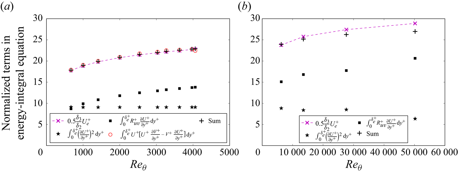
Using direct numerical simulations (DNS) data from Schlatter & Örlü (Reference Schlatter and Örlü2010), we present the terms from the energy integral (2.2) and its approximation (2.4) in figure 1(a). Previous investigations (Laadhari Reference Laadhari2007; Abe & Antonia Reference Abe and Antonia2016; Wei Reference Wei2018) have demonstrated that the viscous dissipation by the mean flow is approximately  $\int _0^{\delta ^+}(\partial U^+/\partial y^+)^2\,{\rm d} y^+ \approx 9$ for turbulent channel, pipe or boundary layer flows over a flat plate, seemingly independent of the Reynolds number. This dissipation by the mean flow occurs mainly in the traditional viscous and buffer layers, where the velocity profile
 $U^+$ exhibits self-similarity with respect to the wall-normal distance
 $y^+$.
Evaluation of the normalized energy integral (2.2) and the approximation (2.4), where the  $+$ symbols represent the sum of the two terms on the right-hand side of (2.4): (a) DNS data of Schlatter & Örlü (Reference Schlatter and Örlü2010); (b) experimental data of Baidya et al. (Reference Baidya, Philip, Hutchins, Monty and Marusic2017, Reference Baidya, Philip, Hutchins, Monty and Marusic2021).

In contrast, the TKE production  $\int _0^{\delta ^+_e} R^+_{uv}(\partial U^+/\partial y^+)\,{\rm d} y^+$ clearly increases with Reynolds number, as shown in figure 1(a). The figure demonstrates that the sum of the two terms on the right-hand side of (2.4) (represented by black
 $+$ symbols) shows excellent agreement with the directly computed value on the left-hand side of the equation (indicated by red circles). Furthermore, the sum also aligns closely with the approximation
 $0.5 \delta _3/\delta _2 U^+_e$ (denoted by magenta
 $\times$ symbols), supporting the validity of the approximate expression in (2.4).
While figure 1(a) exhibits excellent agreement with the approximate (2.4), the DNS data used in the figure are at relatively moderate Reynolds numbers. To assess the applicability of the approximate (2.4) at higher Reynolds numbers, figure 1(b) incorporates data from experiments conducted by Baidya et al. (Reference Baidya, Philip, Hutchins, Monty and Marusic2017, Reference Baidya, Philip, Hutchins, Monty and Marusic2021). In these experiments, the mean wall-normal velocity was not measured, preventing the direct computation of the left-hand side of (2.2) from the experimental data. While the approximate (2.4) shows good agreement at  $Re_\theta \approx 6300$ and 13 000 (or
 $Re_\tau \approx 2500$ and 5000), noticeable deviations are observed at higher Reynolds numbers.
These discrepancies are likely attributed to limitations in experimental resolution, which become increasingly pronounced at higher Reynolds numbers. It is well established that viscous dissipation by the mean shear occurs predominantly in the viscous sub-layer and buffer layer of the ZPG TBL, where TKE production also peaks. To accurately capture dissipation and TKE production in these flows, the viscous sub-layer must be well resolved. However, at high Reynolds numbers, limitations in probe size often result in the first data point falling outside the viscous sub-layer. For example, at  $Re_\theta \approx 28\,000$, the first data point is located at
 $y^+ \approx 8.8$, and at
 $Re_\theta \approx 50\,000$, it is at
 $y^+ \approx 25.6$. This under-resolution in the near-wall region leads to underestimations in the calculated integrals, as seen in figure 1(b).
To further demonstrate the impact of experimental resolution, we artificially coarsened the data for the lowest Reynolds number case by removing the initial data points, thereby shifting the first data point to  $y^+=28.2$. This adjustment parallels the conditions at the highest Reynolds number, where the first data point is at
 $y^+=25.6$. Notably, the calculated integral of viscous dissipation continues to exhibit the same underestimation. For brevity, the figure illustrating this adjustment is not included here.
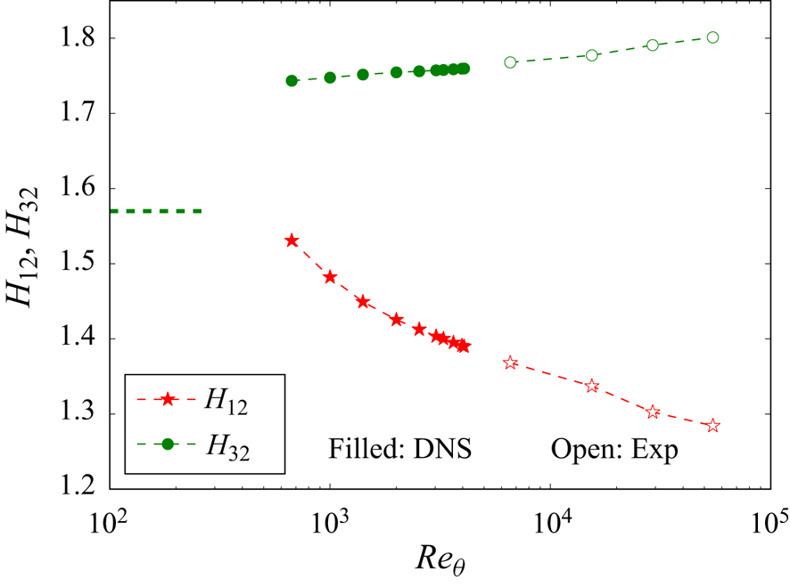
Given the significance of the energy thickness  $\delta _3$ in estimating TKE production, figure 2 shows the variation of the ratio
 $H_{32} = \delta _3/\delta _2$ with Reynolds number in the ZPG TBL. For comparison, the commonly used shape factor
 $H_{12} = \delta _1/\delta _2$ is also included, demonstrating a clear decrease with increasing Reynolds number. In contrast, the ratio
 $H_{32}$ exhibits a slower increase with Reynolds number, indicating a weaker dependence.
The variation of ratio  $H_{32} = \delta _3/\delta _2$ in the ZPG TBL. For laminar flow, the Blasius solution predicts
 $H_{32} \approx 1.57$. Also shown is the commonly used shape factor
 $H_{12}=\delta _1/\delta _2$, with laminar value
 $2.59$, for comparison. The data are from DNS by Schlatter & Örlü (Reference Schlatter and Örlü2010). The experimental data are from Baidya et al. (Reference Baidya, Philip, Hutchins, Monty and Marusic2021).

3. The TBLs under pressure gradient
In this study, we primarily use the DNS data by Coleman, Rumsey & Spalart (Reference Coleman, Rumsey and Spalart2018) to validate our analytical results. The DNS study by Coleman et al. (Reference Coleman, Rumsey and Spalart2018) investigated non-equilibrium TBLs subjected first to an APG and then to an FPG. In their simulations, pressure gradients were induced using a transpiration profile  $V_{top}(x)$ acting through a virtual parallel plane offset by a fixed distance
 $Y$ from the flat no-slip surface. The archived simulation data were normalized by
 $Y$ for length and
 $U_{0}= U_e(x_0)$ for velocity.
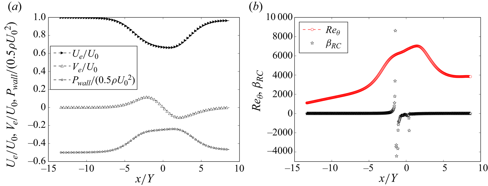
Figure 3 illustrates the streamwise evolution of flow for case C from the DNS data of Coleman et al. (Reference Coleman, Rumsey and Spalart2018). In figure 3(a), the variations of normalized boundary layer edge velocities,  $U_e/U_{0}$ and
 $V_e/U_{0}$, along with normalized wall pressure,
 $P_{wall}/(0.5\rho U_{0}^2)$, are shown. Positive
 $V_e$ is imposed for
 $-10 \lesssim x/Y \leq 0$, transitioning to negative for
 $x/Y > 0$. Analysis of the wall shear stress reveals flow separation in the range
 $-1.4 \lesssim x/Y \lesssim 0.4$. According to DNS pressure gradient data, the FPG region begins near
 $x/Y \approx 0.87$. In the APG region,
 $U_e$ decreases to approximately 66 % of the initial free-stream velocity before increasing again in the FPG region.
(a) Variations of  $U_e$,
 $V_e$ and
 $P_{wall}$ in the DNS study by Coleman et al. (Reference Coleman, Rumsey and Spalart2018). (b) Variations of Reynolds number and
 $\beta _{{RC}}$. To enhance clarity, not all data points along the
 $x$-direction are shown.

Figure 3(b) shows the streamwise variation of the Reynolds number  $Re_\theta = U_e \delta _2/\nu$ and the Rotta–Clauser parameter
 $\beta _{{RC}}$, defined as
 $\beta _{{{RC}}} = (\delta _1/(\rho u^2_\tau ))\,{\rm d} P_e/{\rm d}\kern0.07em x$. In the study of TBLs under pressure gradient, the Rotta–Clauser parameter is commonly used to measure the strength of the pressure gradient (Clauser Reference Clauser1956; Rotta Reference Rotta1962). The value of
 $\beta _{{RC}}$ approaches infinity at the separation points located at
 $x/Y \approx -1.4$ and
 $x/Y \approx 0.4$. The Reynolds number in the simulation ranges from 1000 to 7200, with its peak occurring in the FPG region at
 $x/Y \approx 1.5$.
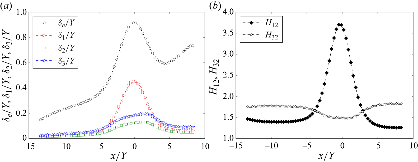
Figure 4(a) presents the variations of the different thicknesses  $\delta _e, \delta _1, \delta _2, \delta _3$ in the
 $x$-direction from the DNS data of Coleman et al. (Reference Coleman, Rumsey and Spalart2018). The figure illustrates that
 $\delta _e$ and
 $\delta _1$ both increase rapidly under APG and decrease rapidly under FPG in their simulations. Meanwhile,
 $\delta _2$ and
 $\delta _3$ also increase under APG and decrease under FPG, but the variation is smaller.
(a) Variations of  $\delta _e, \delta _1, \delta _2, \delta _3$ in the DNS study by Coleman et al. (Reference Coleman, Rumsey and Spalart2018). (b) Variations of the ratios
 $H_{12}$ and
 $H_{32}$. For clarity, not all data points along the
 $x$-direction are shown.

In figure 4(b), the ratios of the thicknesses are presented. The commonly used shape factor in TBL studies,  $H_{12}$, increases under APG and decreases under FPG. Conversely, the ratio
 $H_{32}$ varies oppositely, decreasing under APG and increasing under FPG. These ratios have long been recognized as useful descriptors of velocity profiles (see Schlichting Reference Schlichting1979). If turbulent velocity profiles can be approximated by a one-parameter family of curves, then
 $H_{12}$ and
 $H_{32}$ would be related to each other uniquely (see Schlichting Reference Schlichting1979). For instance, assuming power-law velocity profiles, Wieghardt (Reference Wieghardt1945) proposed the relationship
 $H_{12} = H_{32}/(3H_{32}-4)$ (see also Schlichting Reference Schlichting1979). However, experimental data reveal that the relationship between
 $H_{12}$ and
 $H_{32}$ is not unique, as it is influenced by Reynolds number, pressure gradients and flow history, although the deviation from Wieghardt's approximation remains relatively small.
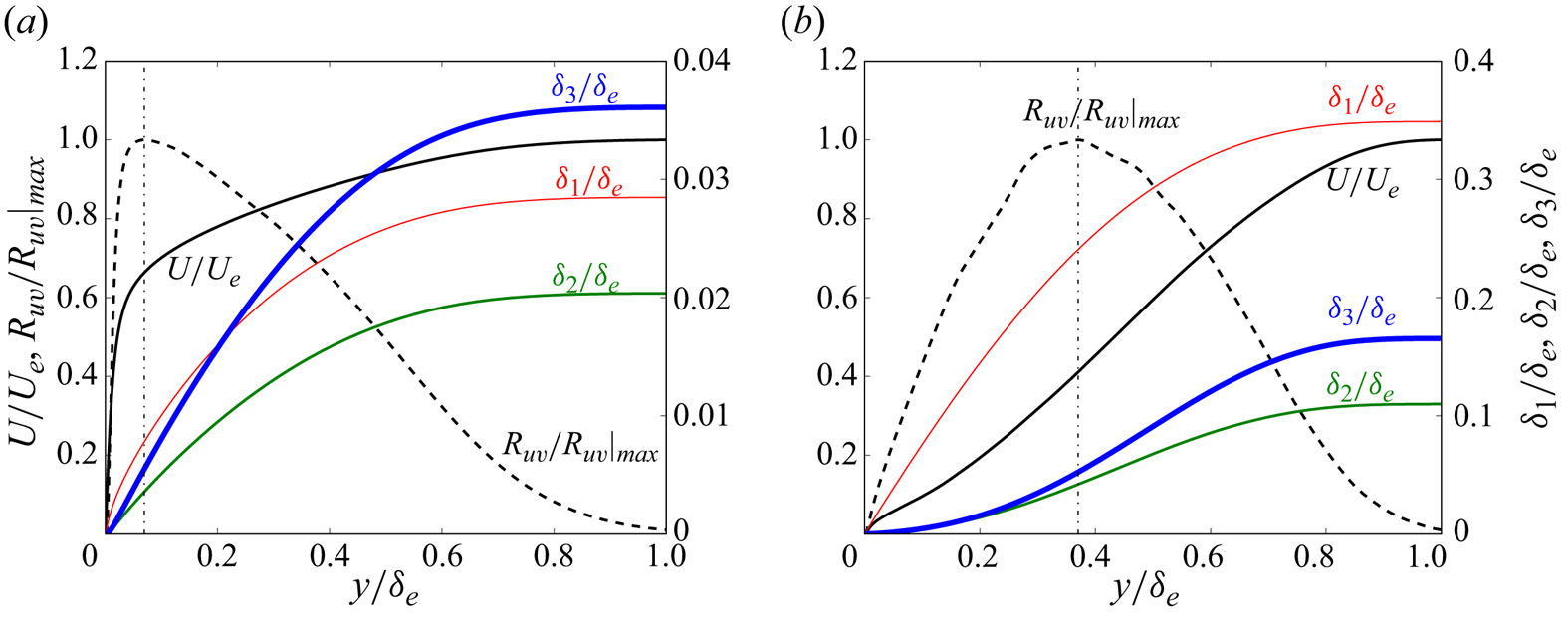
To illustrate the influence of different flow layers, figure 5 shows the cumulative distributions in the calculation of  $\delta _1$,
 $\delta _2$ and
 $\delta _3$. In figure 5(a), the results at
 $x/Y = -10$ are presented, where the pressure gradient is negligible, with
 $Re_\theta \approx 1600$ and
 $\beta _{{RC}} \approx 0.017$. Figure 5(b) shows the results at
 $x/Y = -1.4$, near the separation point, where
 $Re_\theta \approx 6100$ with
 $\beta _{{RC}} \approx -2.9 \times 10^{4}$.
Contributions of different layers to  $\delta _1$,
 $\delta _2$ and
 $\delta _3$: (a) at
 $x/Y=-10$, where the pressure gradient is negligible, with
 $Re_\theta \approx 1600$; (b) at
 $x/Y=-1.44$ near the separation point, where
 $\beta _{{RC}}$ approaches infinity and
 $Re_\theta \approx 6100$. The vertical dash-dotted line indicates the peak Reynolds shear stress location
 $y_m/\delta _e$.

Based on the force balance characteristics in the mean momentum equation, Wei et al. (Reference Wei, Fife, Klewicki and McMurtry2005) proposed a four-layer structure for ZPG TBLs and turbulent channel/pipe flows. The peak location of the Reynolds shear stress,  $y_m$, represents the centre of layer III (the meso layer) and is indicated by a vertical dash-dotted line in the figure.
Equation (1.1a) defines  $\delta _1$ as the integral of the mean streamwise velocity deficit
 $(U_e - U)/U_e$ across the boundary layer, with the velocity deficit reaching its maximum at the wall. Under weak pressure gradients, as shown in figure 5(a), the inner regions contribute minimally to
 $\delta _1$,
 $\delta _2$ and
 $\delta _3$ due to their small fraction of the overall boundary layer thickness. For ZPG TBLs, it is established that
 $y_m \sim 2 \delta _e/\sqrt {Re_\tau }$ (see Afzal Reference Afzal1982; Sreenivasan & Sahay Reference Sreenivasan and Sahay1997; Wei et al. Reference Wei, Fife, Klewicki and McMurtry2005). At
 $x/Y=-10$,
 $y_m/\delta _e \sim 6$ %. In the calculation of
 $\delta _2$ and
 $\delta _3$, the velocity deficit is weighted by
 $U/U_e$ and
 $U/U_e(1+U/U_e)$, respectively. These weighting functions further diminish the contribution of the near-wall region, as
 $U/U_e$ is relatively small in these areas. Due to the different weighting functions,
 $\delta _3$ will be larger than
 $\delta _2$, leading to
 $H_{32}$ being greater than 1.
Under strong APG, the shape of the mean streamwise velocity is influenced significantly, especially in the near-wall region, as shown in figure 5(b). Concurrently, the peak location of Reynolds shear stress,  $y_m$, moves farther from the wall (see Wei & Knopp Reference Wei and Knopp2023), with
 $y_m/\delta _e \approx 0.4$ at this
 $x$-location. In the APG regime, the inner regions where the mean streamwise velocity is strongly affected and contribute significantly to
 $\delta _1$. In contrast, changes in the inner region's velocity profile have less impact on
 $\delta _2$ and
 $\delta _3$. This leads to a substantial variation in the shape factor
 $H_{12}$, as shown in figure 4(b), while the variation in
 $H_{32}$ remains comparatively minor.
In TBL flows, the mass displacement thickness  $\delta _1$ is a key parameter in the integral form of the continuity equation, appearing as
 $V_e = -\delta _e\,{\rm d}U_e/{\rm d}\kern0.07em x + {\rm d}(U_e \delta _1)/{\rm d}\kern0.07em x$ (see Wei et al. Reference Wei, Li, Knopp and Vinuesa2023a,Reference Wei, Li and Wangb), and is linked directly to mass conservation. Similarly, the momentum thickness
 $\delta _2$ arises in the integral of the streamwise momentum equation (i.e. the von Kármán–Pohlhausen equation) as
 ${\rm d}(U^2_e \delta _2)/{\rm d}\kern0.07em x$ (see von Kármán Reference von Kármán1921; Pohlhausen Reference Pohlhausen1921), making it closely tied to momentum transport and wall shear stress in TBLs. In this study, we extend this framework by demonstrating that the energy thickness
 $\delta _3$ appears naturally in the integral of the streamwise momentum equation when multiplied by the velocity
 $U$, in the form
 ${{\rm d}(U_e^3 \delta _3)}/{{\rm d}\kern0.07em x}$. This reveals a close connection between
 $\delta _3$ and the energetic properties of TBLs, offering new insights into energy conversion processes in these flows. By linking energy thickness with TKE production and flow separation, we provide a more comprehensive understanding of boundary layer behaviour, particularly in the presence of pressure gradients.
3.1. Friction coefficient in TBLs under pressure gradients
One of the primary goals in the study of TBLs is predicting the wall shear stress or friction coefficient  $C_f = \tau _{wall}/(0.5 \rho U^2_e) = 2 u^2_\tau /U^2_e$, where
 $\tau _{wall}$ is the local wall shear stress, and
 $U_e$ is the mean streamwise velocity at the boundary layer edge. While accurate prediction models for
 $C_f$ have been developed for ZPG TBLs, predicting
 $C_f$ under pressure gradients, and particularly determining the location where the wall shear stress becomes zero (i.e. the separation point), remains a challenge. Figure 6(a) presents the variations of
 $C_f$ and
 $H_{32}$ in the
 $x$-direction from the DNS data of Coleman et al. (Reference Coleman, Rumsey and Spalart2018). In ZPG TBLs,
 $H_{32}$ exceeds
 $1.7$, and its value increases gradually with Reynolds numbers (see figure 2). However, under APG conditions, the value of
 $H_{32}$ decreases below the ZPG values. Specifically, figure 6(a) demonstrates that the wall shear stress reaches zero at approximately the location where
 $H_{32}$ drops below
 $1.48$.
(a) Variation of friction coefficient  $C_f$ and
 $H_{32}$ using DNS data from Coleman et al. (Reference Coleman, Rumsey and Spalart2018). (b) Comparison of
 $C_f$ and
 $H_{32}$ with DNS data from Coleman et al. (Reference Coleman, Rumsey and Spalart2018) (CRS), from Gungor et al. (Reference Gungor, Maciel, Simens and Soria2016) (GMSS) and from Manhart & Friedrich (Reference Manhart and Friedrich2002) (MF), and experimental data from Skåre & Krogstad (Reference Skåre and Krogstad1994) (SKr), from Schubauer & Klebanoff (Reference Schubauer and Klebanoff1951) (SKl), from Bradshaw (Reference Bradshaw1965, Reference Bradshaw1966) (B; open, mild APG; filled, moderate APG), from Clauser (Reference Clauser1954) (C; open, mild APG; filled, moderate APG), from Ludwieg & Tillmann (Reference Ludwieg and Tillmann1949) (LT) and from Schubauer & Sprangenberg (Reference Schubauer and Sprangenberg1960) (SS; open, ID 4500; filled, ID 4800).

To explore the relationship between  $C_f$ and
 $H_{32}$, we conducted an extensive analysis that included a wide range of experimental data along with DNS data. This comprehensive dataset included equilibrium and streamwise-evolving cases from the compilation by Coles & Hirst (Reference Coles and Hirst1969), with the same identifiers (ID) used for reference. We examined equilibrium TBL flows under mild APG from Bradshaw (Reference Bradshaw1966) (ID 2500) and moderate APG from Bradshaw (Reference Bradshaw1965) (ID 2600). Additionally, we studied equilibrium boundary layer flows under mild APG (ID 2200) and moderate APG (ID 2300) from Clauser (Reference Clauser1954). Streamwise evolving flows under strong APG (ID 1200) from Ludwieg & Tillmann (Reference Ludwieg and Tillmann1949), as well as flows B (ID 4500) and E (ID 4800) from Schubauer & Sprangenberg (Reference Schubauer and Sprangenberg1960), were also part of our analysis. Furthermore, we considered the TBL flow over a large aerofoil-like body from Schubauer & Klebanoff (Reference Schubauer and Klebanoff1950), which involves small surface curvature and history effects. This flow scenario includes an initial phase under a strong FPG in the nose region, transitioning to a mild FPG, and finally encountering an APG region.
In the dataset compiled by Coles & Hirst (Reference Coles and Hirst1969), the boundary layer thickness  $\delta$, the wake factor
 $\varPi$, and the friction velocity
 $u_\tau$ were determined by minimizing the root mean square deviation of the data from the law-of-the-wall/law-of-the-wake:
 \begin{equation} u^+=\frac{1}{\kappa}\log(y^+) + B + \frac{2\varPi}{\kappa}\left(\sin\left(\frac{{\rm \pi}\eta}{2}\right)\right)^2,\quad \eta=\frac{y}{\delta}, \end{equation}
using  $\kappa =0.41$ and
 $B=5.0$. For the calculation of the integral thicknesses, an analytical wall law for the mean velocity was applied between the wall and the first data point, as describe in Coles & Hirst (Reference Coles and Hirst1969).
Figure 6(b) illustrates the variation of  $C_f$ with
 $H_{32}$ under different pressure gradient conditions. It shows that the manner in which the APG is applied influences the rate at which
 $C_f$ decreases with
 $H_{32}$. Nevertheless, the figure clearly indicates that
 $C_f$ approaches zero, signifying the separation point, at
 $H_{32} \approx 1.48$, regardless of the specific method of APG imposition. This consistency suggests that
 $H_{32}$ has potential as a reliable criterion for predicting flow separation.
3.2. Energy integral equation for TBLs under pressure gradients
The energy integral equation for TBLs under arbitrary pressure gradients can be obtained as follows (detailed in Appendix B):
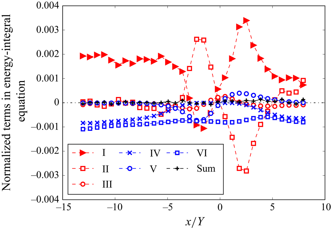
 \begin{align} 0&= \underbrace{\frac{1}{2}\,\frac{{\rm d}}{{\rm d}\kern0.07em x}(U^3_e \delta_3)}_{\text{I}} \underbrace{{}- \int_0^{\delta_e} \left(\frac{1}{\rho}\,\frac{\partial P}{\partial x} + U_e\,\frac{{\rm d} U_e}{{\rm d}\kern0.07em x}\right) U\,{\rm d} y}_{\text{II}} + \underbrace{\frac{{\rm d}}{{\rm d}\kern0.07em x} \int_0^{\delta_e} U R_{uu}\,{\rm d} y}_{\text{III}} \nonumber\\ & \underbrace{{}-\nu \int_0^{\delta_e} \left( \frac{\partial U}{\partial y} \right)^2\,{\rm d} y}_{\text{IV}} \underbrace{{}-\int_0^{\delta_e} R_{uu}\,\frac{\partial U}{\partial x}\,{\rm d} y}_{\text{V}} \underbrace{{}-\int_0^{\delta_e} R_{uv}\,\frac{\partial U}{\partial y}\,{\rm d} y}_{\text{VI}} . \end{align}
Here, the sum of terms  $\mathrm {I}$ and
 $\mathrm {II}$ represents the energy exchange from the mean advective and pressure forces. Term
 $\mathrm {III}$ arises from the gradient of Reynolds normal stress
 ${\partial R_{uu}}/{\partial x}$. Term
 $\mathrm {IV}$ represents the viscous dissipation into internal energy by the mean shear, while terms
 $\mathrm {V}$ and
 $\mathrm {VI}$ are the TKE production terms, i.e. they convert mean kinetic energy to turbulence kinetic energy. In the case of the ZPG TBL, term
 $\mathrm {II}$ vanishes. For the ZPG laminar boundary layer, terms
 $\mathrm {II}, \mathrm {III}, \mathrm {V}, \mathrm {VI}$ are zero, and the Wieghardt equation (1.2) is reproduced.
The terms in (3.2) are illustrated in figure 7 using DNS data from Coleman et al. (Reference Coleman, Rumsey and Spalart2018). The non-smoothness observed in the data for terms I and II can be attributed to the computation of  $x$-derivatives during the post-processing stage. Despite this, the residual remains close to zero, with any deviation likely arising from the calculation of
 $x$-derivatives in the post-processing stage.
Terms in the energy integral (3.2). Data are from DNS data of Coleman et al. (Reference Coleman, Rumsey and Spalart2018). Note that velocity in the DNS data is normalized by the free-stream velocity at the simulation inlet, and distance is normalized by the domain size in the wall-normal direction.

Figure 7 demonstrates that under strong pressure gradients, term  $\mathrm {II}$ becomes significant and cannot be neglected. This observation aligns with the findings in Wei, Li & Wang (Reference Wei, Li and Wang2024), which emphasize the substantial deviation of
 $-\partial (P_{wall}/\rho )/\partial x$ from
 $U_e\,{\rm d}U_e/{\rm d}\kern0.07em x$ under such conditions. Consequently, the original Wieghardt equation (1.2) becomes invalid under strong pressure gradients.
3.3. Approximations for the terms in the energy integral equation
In numerical simulations of TBL, the terms in (3.2) can be determined directly and precisely from the simulation data, assuming that adequate numerical resolutions are employed. However, in physical experiments, the resolution is often constrained, particularly in the vicinity of the wall. Additionally, in typical hot-wire experiments, the number of measurements across various  $x$-stations is limited. Therefore, the development of approximations for the terms in the energy integral equations becomes valuable, particularly for those terms that are difficult to obtain experimentally. Even a rough estimation of the order of magnitude would be useful for gaining further insights. Moreover, an investigation of the scaling of the different terms using characteristic boundary layer quantities is of interest. The goal is to reveal boundary layer parameters other than the popular parameters like
 $H_{12}$, which characterize the local state of the boundary layer and how susceptible the flow is to flow separation.
To gain a better understanding of the terms in (3.2), we first analyse the effects of the pressure gradient on the shapes of the mean flow and Reynolds stresses in the wall-normal direction. Subsequently, we present the distribution of the variables within the integrals in (3.2), allowing us to appreciate the contributions of different regions of the TBL to the overall integrals.
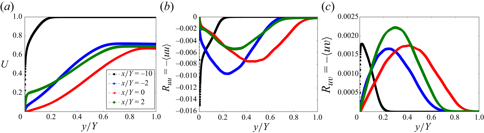
The pressure gradient directly affects the shape of the mean flow and the distribution of Reynolds stresses. Figure 8 illustrates the variations in mean streamwise velocity  $U$, Reynolds normal stress
 $R_{uu}$, and Reynolds shear stress
 $R_{uv}$ at four distinct
 $x$-locations, each experiencing different intensities of pressure gradients. Under zero or weak pressure gradients,
 $U$ exhibits a steep slope in the near-wall region. The magnitudes of Reynolds normal or shear stresses also peaks in the near-wall region. However, under strong APG, the slope of
 $U$ in the near-wall region diminishes significantly, becoming zero at the separation point. The peak locations of the Reynolds stresses also shift towards the centre of the TBL (see also Wei & Knopp Reference Wei and Knopp2023).
Effects of varying pressure gradients on the profiles of  $U$,
 $R_{uu}$ and
 $R_{uv}$. The Reynolds number and Rotta–Clauser parameters at the four
 $x$-stations are (
 $Re_\theta =1620$,
 $\beta _{{RC}}=0.017$), (
 $Re_\theta = 5770$,
 $\beta _{{RC}}=157$), (
 $Re_\theta =6600$,
 $\beta _{{RC}}=-147$) and (
 $Re_\theta =6800$,
 $\beta _{{RC}}=-23$) for
 $x/Y=-10, -2, 0, 2$, respectively. The DNS data are from Coleman et al. (Reference Coleman, Rumsey and Spalart2018).

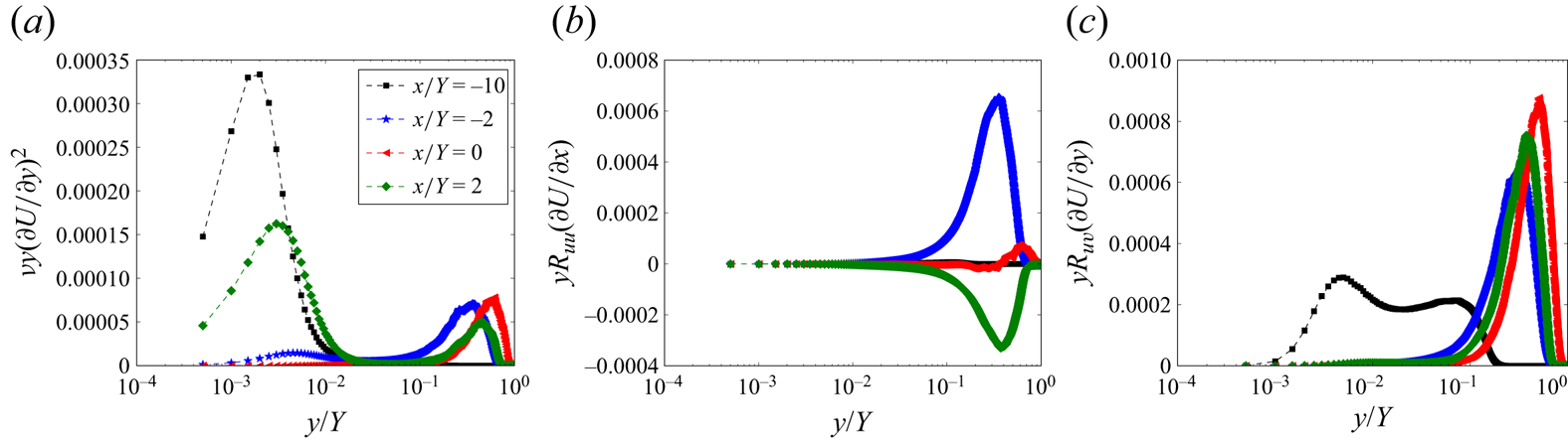
The variations in the mean flow and Reynolds stress profiles, induced by pressure gradients, lead to significant changes in the contributions of different regions within the TBL to dissipation and TKE production. To better show the near-wall region, figure 9 depicts the pre-multiplied dissipation and TKE productions plotted on semi-logarithmic axes. Under weak pressure gradients, the viscous dissipation is concentrated predominantly in the near-wall region, specifically the viscous and buffer sub-layers. However, under strong APG, the viscous dissipation shifts significantly to the outer region, due to the diminishing slope of the mean velocity profile  $U$ in the near-wall region. Analogously, the contribution of the outer region to TKE production also gains prominence under strong APG conditions due to the increase of
 $\partial U/\partial y$ in the case of a large mean-velocity deficit in the outer layer (Gungor et al. Reference Gungor, Maciel, Simens and Soria2016; Maciel et al. Reference Maciel, Wei, Gungor and Simens2018)
(a) Pre-multiplied viscous dissipation profiles. To enhance visibility, the values at  $x/Y=-2$,
 $0$ and 2 have been multiplied by a factor of 10, due to their actual values being significantly smaller compared to that at
 $x=-10$. (b) Pre-multiplied TKE production by
 $R_{uu}\,\partial U/\partial x$. (c) Pre-multiplied TKE production by
 $R_{uv}\,\partial U/\partial y$. The DNS data are from Coleman et al. (Reference Coleman, Rumsey and Spalart2018).

It is well known that the inner normalized mean streamwise velocity  $U^+(y^+)$ in the ZPG TBL exhibits a self-similarity in the viscous and buffer layers (see Tennekes & Lumley Reference Tennekes and Lumley1972; Monin & Yaglom Reference Monin and Yaglom1965). Hence the viscous dissipation term in the ZPG TBL can be estimated as
 \begin{align} \nu \int_0^{\delta_e} (\partial U/\partial y)^2\,{\rm d} y = u^3_\tau \int_0^{\delta^+_e} (\partial U^+{/}\partial y^+)^2\,{\rm d} y^+\approx u^3_\tau \int_0^{20} (\partial U^+{/}\partial y^+)^2\,{\rm d} y^+\approx {c}\, u^3_\tau. \end{align}
The constant turns out to be approximately 9 (see figure 1). However, under pressure gradients, the inner-scaled  $U^+$ is not self-similar in the near-wall region. Moreover, the dissipation by the mean shear is not concentrated in the near-wall region either. Figure 7 reveals that term
 $\mathrm {IV}$ decreases with the magnitude of the wall shear stress, eventually approaching zero in the separated region (
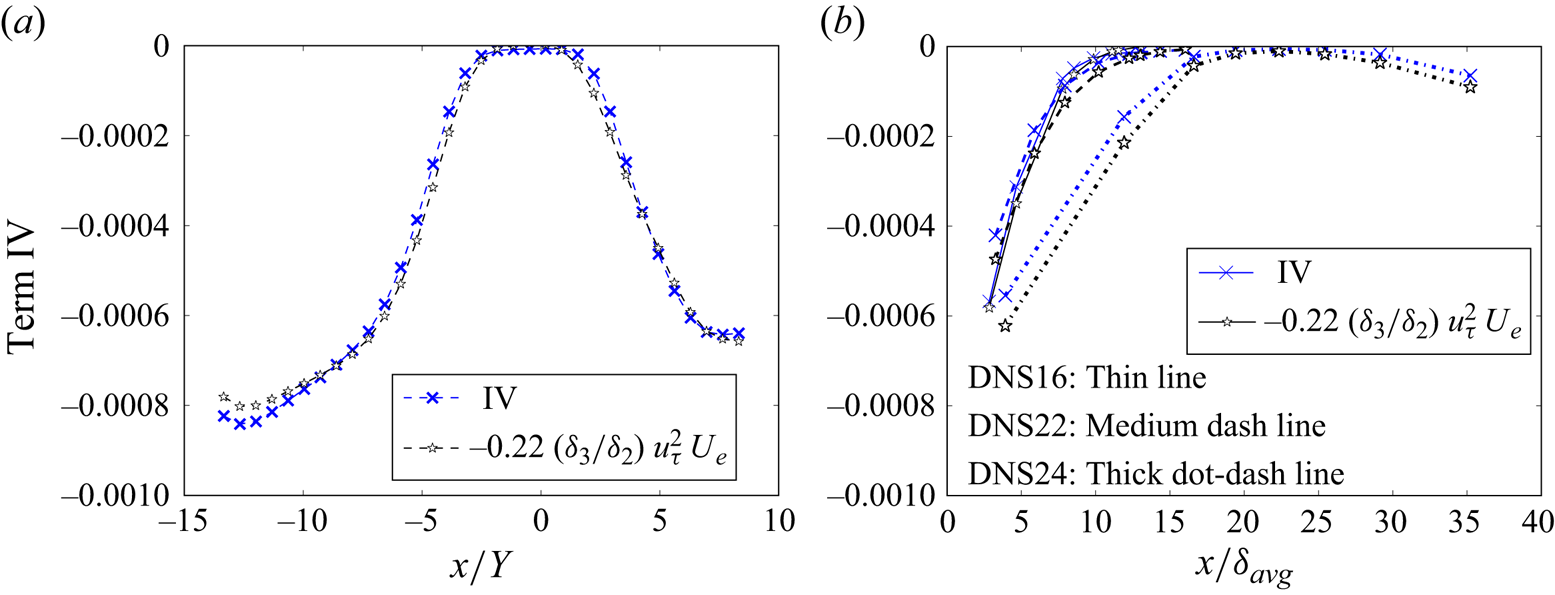
 $-1.4 \lesssim x/Y \lesssim 0.4$). Based on the DNS data of Coleman et al. (Reference Coleman, Rumsey and Spalart2018) shown in figure 10(a), the viscous dissipation by the mean shear can be approximated as
 \begin{equation} {-}\nu \int_0^{\delta_e} \left( \frac{\partial U}{\partial y}\right)^2{\rm d} y \sim{-}0.22\, \frac{\delta_3}{\delta_2}\,u^2_\tau U_e. \end{equation}
To further assess the validity of the approximation (3.4), figure 10(b) presents data from independent DNS studies by Gungor, Maciel and colleagues (Gungor et al. Reference Gungor, Maciel, Simens and Soria2016; Gungor, Maciel & Gungor Reference Gungor, Maciel and Gungor2022; Gungor, Gungor & Maciel Reference Gungor, Gungor and Maciel2024). These studies included three simulations of highly non-equilibrium TBLs evolving under a pressure gradient. The publicly accessible data comprise information at eight streamwise positions for each simulation. As figure 10(b) illustrates, the approximation (3.4) exhibits good agreement with the three datasets. However, the underlying physical rationale for this empirical approximation (3.4) remains elusive. Notably, the functional form of (3.4) exhibits a resemblance to the left-hand side of (2.3), suggesting potential connections or analogies between the two expressions. Further investigation is warranted to elucidate the physical basis of this approximation and its applicability in various flow conditions.
Molecular dissipation by mean shear term: (a) DNS data of Coleman et al. (Reference Coleman, Rumsey and Spalart2018); (b) DNS data of Gungor et al. (Reference Gungor, Maciel, Simens and Soria2016, Reference Gungor, Maciel and Gungor2022, Reference Gungor, Gungor and Maciel2024).

To gain insight into and compare the TKE production terms  $\mathrm {V}$ and
 $\mathrm {VI}$, figure 11(a) presents the ratio between
 $V_e$ and
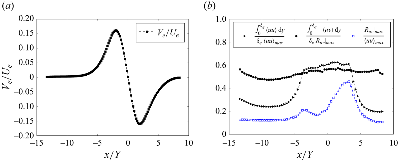
 $U_e$ obtained from the DNS data of Coleman et al. (Reference Coleman, Rumsey and Spalart2018). Figure 11(b) presents the ratios between the averaged Reynolds normal stress and Reynolds shear stress to the maximum Reynolds stresses. Under zero or weak pressure gradients, the mean wall-normal velocity
 $V_e$ is significantly smaller than the streamwise velocity
 $U_e$, resulting in a very small
 $V_e/U_e$ ratio. This indicates that the boundary layer remains thin. However, under strong pressure gradients,
 $V_e$ approaches the magnitude of
 $U_e$, as shown in figure 11(a).
(a) Ratio of  $V_e$ to
 $U_e$ obtained from the DNS data of Coleman et al. (Reference Coleman, Rumsey and Spalart2018). (b) Ratios of the average Reynolds normal stress and Reynolds shear stress to the maximum Reynolds shear stress.

Figure 11(b) demonstrates that, regardless of the pressure gradient, the averaged Reynolds shear stress remains approximately half of the maximum Reynolds shear stress. However, the ratio between the averaged Reynolds normal stress  $\langle uu \rangle$ and
 $\langle uu \rangle _{max}$ exhibits a dependence on the pressure gradient. Specifically, under a weak pressure gradient, this ratio is approximately 0.24. Near the separation point, this ratio increases to approximately 0.6. Furthermore, the ratio between the maximum Reynolds shear stress and
 $\langle uu \rangle _{max}$ also exhibits a pressure gradient dependence. Under weak pressure gradients, this ratio is approximately 0.12, but it can increase to approximately 0.5 under strong pressure gradients. Despite these variations, figure 11(b) illustrates that
 $\langle uu \rangle _{max}$ remains of the same order of magnitude as the maximum Reynolds shear stress. It is noteworthy that in high Reynolds number ZPG TBLs, the maximum Reynolds shear stress is approximately
 $u^2_\tau$.
Figure 7 illustrates that term  $\mathrm {V}$ in (3.2), representing the TKE ‘production’ by
 $R_{uu} \partial U/\partial x$, is insignificant under weak pressure gradients. However, under strong pressure gradients and significant streamwise changes of the wall shear stress, this term approaches the magnitude of the production resulting from
 $R_{uv}\,\partial U/\partial y$. On the other hand, for flows near equilibrium with a small streamwise change of the wall shear stress, the contribution is much smaller, as shown in figure 9 of Skåre & Krogstad (Reference Skåre and Krogstad1994). Furthermore, term
 $\mathrm {V}$ becomes positive under strong FPG, indicating a conversion of TKE to mean kinetic energy. The sum of terms
 $\mathrm {V}$ and
 $\mathrm {VI}$ remains negative, indicating an overall net conversion of mean kinetic energy into TKE across the entire domain of the DNS conducted by Coleman et al. (Reference Coleman, Rumsey and Spalart2018).
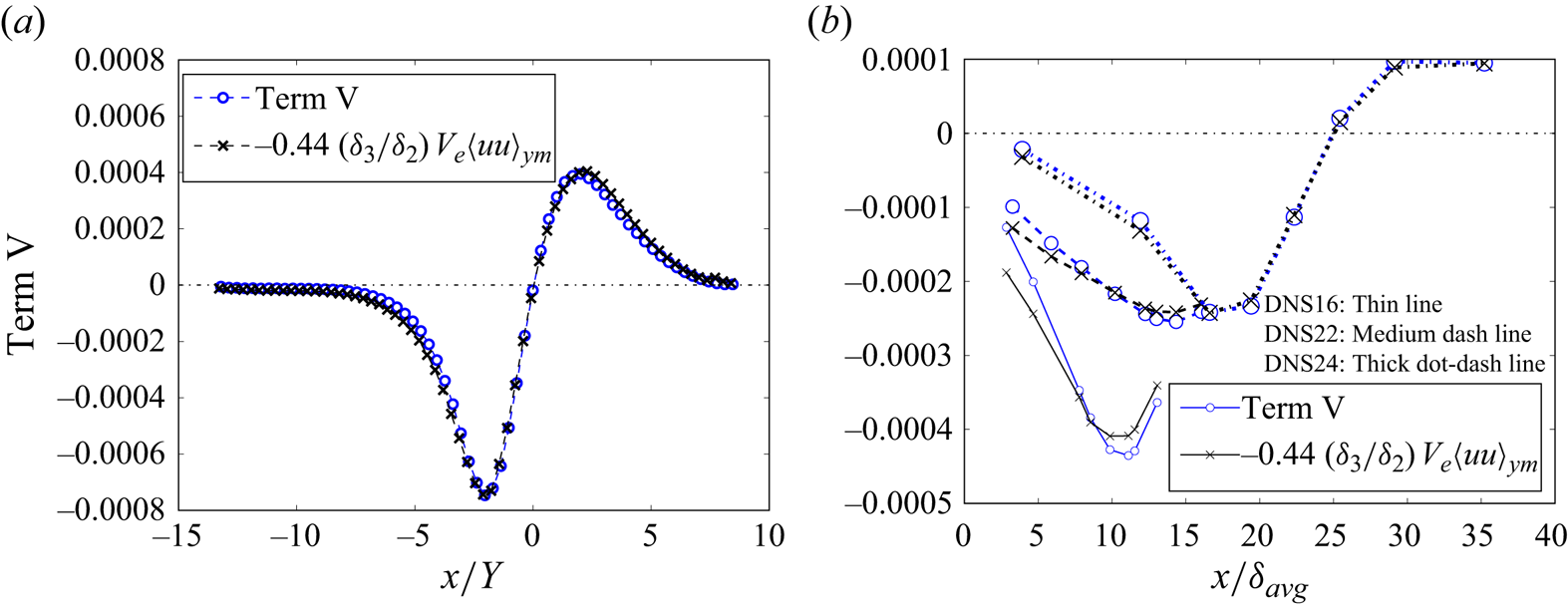
Based on the DNS data of Coleman et al. (Reference Coleman, Rumsey and Spalart2018) shown in figure 12, the term  $\mathrm {V}$ in (3.2) can be approximated as
 \begin{equation} -\int_0^{\delta_e} R_{uu}\,\frac{\partial U}{\partial x}\,{\rm d} y = \int_0^{\delta_e} R_{uu}\, \frac{\partial V}{\partial y}\,{\rm d} y \approx{-}0.44\,\frac{\delta_3}{\delta_2}\,{V_e} \langle uu \rangle_{y_m}. \end{equation}
Approximation of the TKE production from  $R_{uu}\,\partial U/\partial x$: (a) DNS data of Coleman et al. (Reference Coleman, Rumsey and Spalart2018); (b) DNS data of Gungor et al. (Reference Gungor, Maciel, Simens and Soria2016, Reference Gungor, Maciel and Gungor2022, Reference Gungor, Gungor and Maciel2024).

Figure 12(b) shows that the approximate (3.5) also works reasonably well for the DNS data of Gungor et al. (Reference Gungor, Maciel, Simens and Soria2016, Reference Gungor, Maciel and Gungor2022, Reference Gungor, Gungor and Maciel2024). This approximation underscores the significance of  $V_e$ and
 $\langle uu \rangle _{y_m}$, as well as the importance of the thicknesses
 $\delta _2, \delta _3$, in estimating the TKE production by
 $R_{uu}\,\partial U/\partial x$.
Under weak pressure gradients, where  $V_e$ is significantly smaller than
 $U_e$ as shown in figure 11(a), the TKE production by
 $R_{uu}\,\partial U/\partial x$ is therefore considerably smaller than that by
 $R_{uv}\,\partial U/\partial y$. However, under strong pressure gradients, the magnitudes of
 $V_e$ and
 $U_e$ become comparable. Additionally, as shown in figure 11(b),
 $\int _0^{\delta _e} \langle uu \rangle \,{\rm d} y$ is larger than
 $\int _0^{\delta _e} R_{uv}\,{\rm d} y$. Consequently, under strong pressure gradients, the TKE production by
 $R_{uu}\,\partial U/\partial x$ becomes comparable in magnitude to that from
 $R_{uv}\,\partial U/\partial y$, as shown in figure 7.
Figure 7 shows that term  $\mathrm {VI}$, the integral of TKE production by
 $R_{uv}\,\partial U/\partial y$, exhibits relatively small variations throughout the simulation domain, despite the presence of substantial changes in the pressure gradient. Notably, term
 $\mathrm {VI}$ remains negative across different pressure gradients, indicating that it extracts energy from the mean flow to TKE. Furthermore, figure 13 indicates that the TKE production under weak pressure gradients by
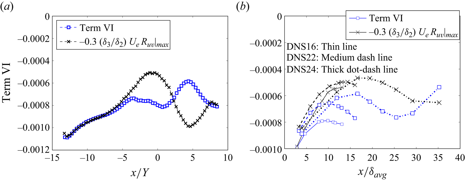
 $R_{uv}\,\partial U/\partial y$ can be estimated as
 \begin{equation} - \int_0^{\delta_e} R_{uv}\,\frac{\partial U}{\partial y}\,{\rm d} y \sim{-}0.3\, \frac{\delta_3}{\delta_2}\,{U_e}\,R_{uv}|_{max}. \end{equation}
However, this estimation loses validity under strong pressure gradients. Nonetheless, it still provides a reasonable estimate of the order of magnitude of the TKE production by  $R_{uv}\,\partial U/\partial y$, as corroborated by independent DNS data from Gungor et al. (Reference Gungor, Maciel, Simens and Soria2016, Reference Gungor, Maciel and Gungor2022, Reference Gungor, Gungor and Maciel2024). Additionally, validation with experimental data from Skåre & Krogstad (Reference Skåre and Krogstad1994) shows excellent support for the approximation in (3.6), with the numerical factor varying between 0.3 and 0.35 across seven
 $x$-stations, averaging 0.32.
Estimation of TKE production by  $R_{uv}\,\partial U/\partial y$: (a) DNS data of Coleman et al. (Reference Coleman, Rumsey and Spalart2018); (b) DNS data of Gungor et al. (Reference Gungor, Maciel, Simens and Soria2016, Reference Gungor, Maciel and Gungor2022, Reference Gungor, Gungor and Maciel2024).

3.4. Normalization of the energy integral equation
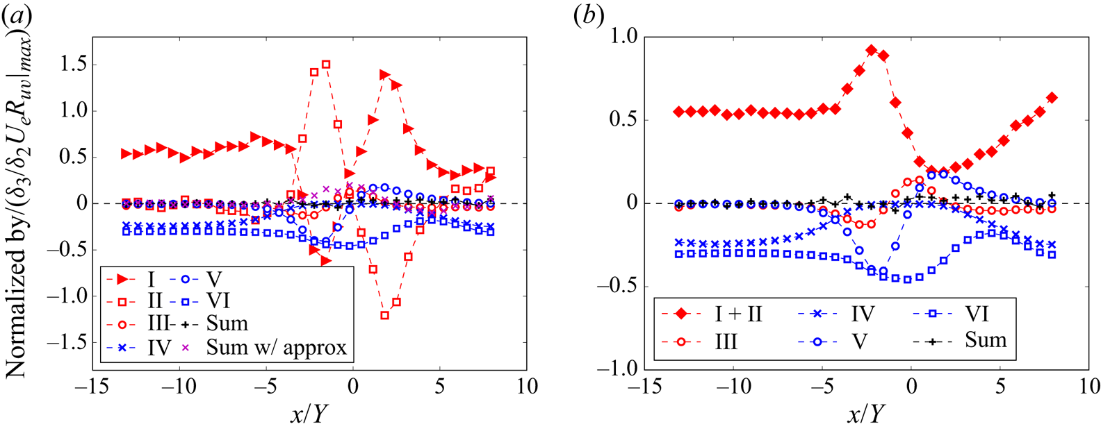
In approximating the terms in the energy integral equation (§ 3.3), the factor  $(\delta _3/\delta _2)U_e\,R_{uv}|_{max}$ assumes a crucial role. This scaling factor can be used effectively to normalize the energy integral (3.2). The outcomes of this normalization are displayed in figure 14, providing a clearer visualization of the relative contributions of the various terms within the equation. In figure 14(a), the black
 $+$ symbols represent the direct sum of terms I–VI calculated using DNS data, while the magenta
 $\times$ symbols represent the sum where terms IV, V and VI are approximated using (3.4), (3.5) and (3.6), respectively. The approximate sum closely aligns with zero under weak pressure gradients, but exhibits notable deviations under strong pressure gradients, primarily due to the limitations of the approximate equation (3.6) in such conditions.
(a) Energy integral equation (3.2) normalized by  $(\delta _3/\delta _2) U_e\,R_{uv}|_{max}$. Black + symbols represent the sum of terms I–VI calculated using DNS data, whereas magenta x symbols represent the sum of terms I–III calculated using DNS data and terms IV–VI estimated using approximate equations. (b) Combined contributions of terms
 $\mathrm {I}$ and
 $\mathrm {II}$. The DNS data are from Coleman et al. (Reference Coleman, Rumsey and Spalart2018).

To further elucidate the combined effect of the advective term and pressure term, terms  $\mathrm {I}$ and
 $\mathrm {II}$ are combined in figure 14(b). Both figures demonstrate that the normalized terms are of or smaller than
 $O(1)$, indicating their relative magnitudes and significance within the energy integral equation.
Under zero or weak pressure gradient, the normalized term  $\mathrm {I}$ approximates
 $0.5$, which aligns with the left-hand side of (2.3). Note that in high Reynolds number ZPG TBLs, the maximum Reynolds shear stress
 $R_{uv}|_{max}$ closely approximates the square of the friction velocity
 $u^2_\tau$.
Figure 14(b) shows that in the presence of strong APG, the advective and pressure forces (sum of terms I and II in (3.2)) augment the injection of mechanical energy into the flow. This additional energy is then converted to TKE mainly by the term  $R_{uu}\,\partial U/\partial x$ (term V). Conversely, under strong FPG (
 $0.2 \lesssim x/Y \lesssim 5$), there is a noticeable decrease in the injection of the mechanical energy, leading to a corresponding reduction in TKE production by
 $R_{uv}\,\partial U/\partial y$ (term VI). Moreover, the term
 $R_{uu}\,\partial U/\partial x$ (term V) reverses its role, converting TKE back to mechanical energy under strong FPG.
Utilizing the scaling factor, the relative contribution of the viscous dissipation term  $\mathrm {IV}$ is related to the ratio
 $u^2_\tau /R_{uv}|_{max}$. Under strong APG, particularly in proximity to the separation point, this ratio undergoes a substantial decrease, resulting in a significant reduction in the viscous dissipation. The contribution of the normalized term
 $\mathrm {V}$ can be assessed by the factor
 $V_e/U_e$, which typically remains negligible small, except in regions under strong pressure gradients.
4. Summary
In this work, we have derived a novel energy integral equation for zero pressure gradient (ZPG) turbulent boundary layers (TBLs). This equation introduces a precise approximation of the combined dissipation resulting from mean shear and TKE production, formulated as  $0.5 (\delta _3/\delta _2) u^2_\tau U_e$. This approximation, free from
 $x$-derivatives, offers a practical alternative for estimating TKE production in physical experiments, where the measurements are typically limited to select
 $x$-stations, and the direct measurement of Reynolds shear stress can be challenging. The accuracy and robustness of our newly derived approximate equation for ZPG TBLs have been validated through comprehensive comparisons with the DNS and experimental data across a wide range of Reynolds numbers.
For TBLs subjected to pressure gradients, the significance of the energy thickness becomes more prominent. Our analysis of multiple independent DNS and experimental datasets, encompassing TBLs under various pressure gradients, reveals a consistent and robust correlation between the friction coefficient  $C_f$ and the ratio
 $H_{32}=\delta _3/\delta _2$. This correlation highlights the potential of using
 $H_{32}$ as an alternative, readily obtainable parameter in predicting flow separation under strong adverse pressure gradients. In addition, we have rigorously derived a novel energy integral equation for the TBL under arbitrary pressure gradients, where
 $\delta _3$ retains its significance. The behaviour of all the terms in the energy integral equation for the TBL under varying pressure gradients is investigated by using high-fidelity DNS data. Furthermore, to enhance practical applicability, we propose approximate equations for the dissipation due to the mean shear and TKE productions resulting from Reynolds normal and shear stresses, explicitly incorporating
 $\delta _3$. The accuracy and reliability of these approximate equations are confirmed through validation against diverse DNS datasets.
Our investigation also reveals that under mild pressure gradients, the TKE production by  $R_{uu}\, \partial U/\partial x$ is negligible compared to that by
 $R_{uv}\,\partial U/\partial y$. However, in the presence of strong pressure gradients, the production by
 $R_{uu}\,\partial U/\partial x$ becomes comparable in magnitude to that by
 $R_{uv}\,\partial U/\partial y$. While the TKE production by
 $R_{uv}\,\partial U/\partial y$ remains consistently positive under all pressure gradients, the production by
 $R_{uu}\,\partial U/\partial x$ reverses sign under a strong favourable pressure gradient, indicating a conversion of TKE to mean kinetic energy. These observations provide valuable insights into the intricate physics governing TBLs under pressure gradients, advancing our understanding of their behaviour and dynamics.
Acknowledgements
We express our gratitude to Dr Coleman, Dr Gungor, and Dr Maciel for generously sharing their DNS data. The DNS dataset from Coleman et al. (Reference Coleman, Rumsey and Spalart2018) is archived in the NASA Turbulence Modeling Resource (TMR) at https://turbmodels.larc.nasa.gov/Other_DNS_Data/separation_bubble_2d.html.
Declaration of interests
The authors report no conflict of interest.
Appendix A. Derivation of the energy integral equation for ZPG TBLs
The advective terms in the mean momentum equation, when multiplied by  $U$, yield
 \begin{equation} {-}U \left[U\,\frac{\partial U}{\partial x} + V\,\frac{\partial U}{\partial y} \right] = U \left[U\, \frac{\partial V}{\partial y} - V\,\frac{\partial U}{\partial y} \right] = \frac{3}{2}\,U^2\, \frac{\partial V}{\partial y} - \frac{1}{2}\,\frac{\partial (U^2V)}{\partial y}. \end{equation}
The integral of the second term on the right-hand side is trivial. To obtain the integral of the first term on the right-hand side, we first transform the equation into a dimensionless form using the normalized variables defined as (see Wei et al. Reference Wei, Li and Wang2023b)
 \begin{equation} U^-\equiv \frac{U_e - U}{U_e}, \quad V^-\equiv \frac{V}{V_e}, \quad y^-\equiv \frac{y}{\delta_e}. \end{equation}
Substituting the normalized variables, the term  $U^2\,\partial V/\partial y$ can be expressed as
 \begin{equation} U^2\,\frac{\partial V}{\partial y} = \frac{U^2_e V_e}{\delta_e} \left(1- 2 U^-+ (U^-)^2 \right)\frac{\partial V^-}{\partial y^-}. \end{equation}
Wei et al. (Reference Wei, Li and Wang2023b) derived an approximate equation for
 \begin{equation} \frac{\partial V^-}{\partial y^-} \approx{-}\frac{\delta_e}{\delta_1}\,y^-\,\frac{\partial U^-}{\partial y^-}, \end{equation}
which transforms the above equation to
 \begin{align} U^2\,\frac{\partial V}{\partial y} &\approx{-} \frac{U^2_e V_e}{\delta_1} \left\{ \frac{\partial }{\partial y^-}(y^- U^-) - U^-{-} \frac{\partial }{\partial y^-}(y^- (U^-)^2) + (U^-)^2 \right.\nonumber\\ &\quad \left. {}+ \frac{1}{3}\,\frac{\partial }{\partial y^-}(y^- (U^-)^3) - \frac{1}{3}\,(U^-)^3 \right\}. \end{align}
Using the approximate (A5), the integral of (A1) from  $y=0$ to
 $y=\delta _e$ becomes
 \begin{align} & -\int_0^{\delta_e} U \left[U\,\frac{\partial U}{\partial x} + V\,\frac{\partial U}{\partial y} \right]{\rm d} y = \int_0^{\delta_e} \frac{3}{2}\,U^2\,\frac{\partial V}{\partial y}\,{\rm d} y - \int_0^{\delta_e} \frac{1}{2}\,\frac{\partial (U^2V)}{\partial y}\,{\rm d} y \nonumber\\ &\quad \approx{-}\frac{3}{2}\,U^2_eV_e\,\frac{ \delta_e}{\delta_1} \left( -\int_0^1 (U^-)\,{\rm d} y^-+ \int_0^1 (U^-)^2\,{\rm d} y^-{-} \frac{1}{3} \int_0^1 (U^-)^3\,{\rm d} y^- \right) - \frac{1}{2}\, U^2_e V_e \nonumber\\ &\quad ={-}\frac{3}{2}\,U^2_eV_e\,\frac{ \delta_e}{\delta_1} \left( - \frac{\delta_1}{\delta_e} + \frac{\delta_1 - \delta_2}{\delta_e} - \frac{1}{3}\,\frac{\delta_1 + \delta_3 - 3\delta_2}{\delta_e} \right) - \frac{1}{2}\,U^2_e V_e \nonumber\\ &\quad = \frac{1}{2}\,\frac{\delta_3}{\delta_1}\,U^2_e V_e. \end{align}
Wei & Klewicki (Reference Wei and Klewicki2016, Reference Wei and Klewicki2023) have found that  $U_e V_e$ at high Reynolds numbers of ZPG TBLs can be approximated as
 \begin{equation} U_e V_e \approx H_{12} u^2_\tau, \end{equation}
which leads to an approximation
 \begin{equation} -\int_0^{\delta_e} U \left[U\,\frac{\partial U}{\partial x} + V\,\frac{\partial U}{\partial y} \right]{\rm d} y \approx \frac{1}{2}\,\frac{\delta_3}{\delta_2}\,u^2_\tau U_e. \end{equation}
This approximation equation is supported by the DNS data of Schlatter & Örlü (Reference Schlatter and Örlü2010), as shown in figure 1. This suggests a close relationship between the energy input from the advective force in the streamwise direction and parameters such as the energy thickness and momentum thickness, as well as the wall shear stress  $u^2_\tau$ and
 $U_e$.
Appendix B. Derivation for the energy integral equation in the  $x$-direction for a TBL under a pressure gradient

The derivation of the energy integral for a TBL under a pressure gradient is more tedious, but the steps are the same. We start with the mean momentum equation for a TBL under a pressure gradient (see Wei et al. Reference Wei, Li and Wang2024):
 \begin{equation} 0 ={-}\left[U\,\frac{\partial U}{\partial x} + V\,\frac{\partial U}{\partial y} \right] + \nu\, \frac{\partial^2 U}{\partial y^2} - \frac{1}{\rho}\,\frac{\partial P}{\partial x} + \frac{\partial R_{uv}}{\partial y} + \frac{\partial R_{uu}}{\partial x}. \end{equation}
In a TBL under zero or weak pressure gradients, the term  $\partial R_{uu}/\partial x$ is typically negligible. However, under a strong APG, it becomes non-negligible.
The energy integral equation is obtained by multiplying the  $x$-momentum equation by
 $U$ and integrating from
 $y=0$ to
 $y=\delta _e$. The integration of the viscous and Reynolds shear stress terms is straightforward. Utilizing integration by parts and the Leibniz integral rule, the integral
 $\int _0^{\delta _e} (U\,{\partial R_{uu}}/{\partial x})\, \mathrm {d} y$ can be expressed as
 \begin{align} \int_0^{\delta_e} U\,\frac{\partial R_{uu}}{\partial x}\,{\rm d} y & = \int_0^{\delta_e} \frac{\partial (U R_{uu})}{\partial x}\,{\rm d} y - \int_0^{\delta_e} R_{uu}\,\frac{\partial U}{\partial x}\,{\rm d} y \nonumber\\ & = \frac{{\rm d}}{{\rm d} x} \int_0^{\delta_e} U R_{uu}\,{\rm d}\kern0.07em x - \int_0^{\delta_e} R_{uu}\, \frac{\partial U}{\partial x}\,{\rm d} y, \end{align}
which corresponds to terms  $\mathrm {III}$ and
 $\mathrm {V}$ in (3.2).
The integral  $\int _0^{\delta _e} -U[U\,\partial U/\partial x + V\,\partial U/\partial y]\,{\rm d} y$ can be expressed as
 \begin{align} & \int_0^{\delta_e} -U \left[ U\,\frac{\partial U}{\partial x} + V\,\frac{\partial U}{\partial y} \right]{\rm d} y ={-}\int_0^{\delta_e} U^2\,\frac{\partial U}{\partial x}\,{\rm d} y + \frac{1}{2} \int_0^{\delta_e} \frac{\partial U^2}{\partial y} \left( \int_0^y \frac{\partial U}{\partial x}\,{\rm d} y' \right){\rm d} y \nonumber\\ &\quad ={-}\int_0^{\delta_e} U^2\,\frac{\partial U}{\partial x}\,{\rm d} y + \frac{1}{2} \int_0^{\delta_e} \frac{\partial}{\partial y} \left(U^2 \int_0^y \frac{\partial U}{\partial x}\,{\rm d} y' \right){\rm d} y - \frac{1}{2} \int_0^{\delta_e} U^2\,\frac{\partial U}{\partial x}\,{\rm d} y \nonumber\\ &\quad ={-} \frac{1}{2} \int_0^{\delta_e} \frac{\partial U^3}{\partial x}\,{\rm d} y + \frac{1}{2}\,U^2_e \int_0^{\delta_e} \frac{\partial U}{\partial x}\,{\rm d} y \nonumber\\ &\quad ={-} \frac{1}{2}\,\frac{{\rm d}}{{\rm d}\kern0.07em x} \int_0^{\delta_e} U^3\,{\rm d} y + \frac{1}{2}\, U^2_e\,\frac{{\rm d}}{{\rm d}\kern0.07em x} \int_0^{\delta_e} U\,{\rm d} y \nonumber\\ &\quad ={-} \frac{1}{2}\,\frac{{\rm d}}{{\rm d}\kern0.07em x} (U^3_e (\delta_e - \delta_1 - \delta_3)) + \frac{1}{2}\,U^2_e\,\frac{{\rm d}}{{\rm d}\kern0.07em x} (U_e(\delta_e - \delta_1)) \nonumber\\ &\quad = \frac{1}{2}\,\frac{{\rm d}(U^3_e \delta_3)}{{\rm d}\kern0.07em x} - U_e\,\frac{{\rm d}U_e}{{\rm d}\kern0.07em x} \int_0^{\delta_e} U\,{\rm d} y. \end{align}
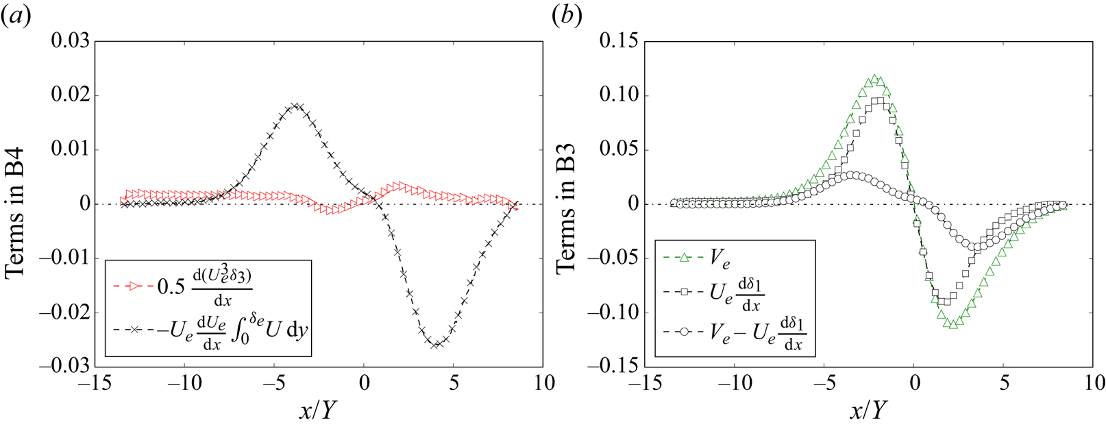
Note that the integration by parts rule was applied to the second integral on the first line. Figure 15(a) illustrates the two components on the right-hand side of (B3). Under a weak pressure gradient, the second component is nearly zero and smaller than the first component. However, under a strong pressure gradient, the magnitude of the second component becomes significantly larger, exceeding that of the first component more than tenfold.
(a) Two components on the right-hand side of (B3). (b) Plots of  $V_e$ and
 $U_e\,{\rm d}\delta _1/{\rm d}\kern0.07em x$. Data are from DNS of Coleman et al. (Reference Coleman, Rumsey and Spalart2018).

It can be shown that the second component on the right-hand side of (B3) is closely related to the pressure gradient and wall-normal flow in the TBL. Recently, Wei et al. (Reference Wei, Li, Knopp and Vinuesa2023a) derived an analytical equation for  $V_e$ in TBL flows under pressure gradient as follows:
 \begin{equation} V_e ={-} \delta_e\,\frac{{\rm d}U_e}{{\rm d}\kern0.07em x} + \frac{{\rm d}(U_e \delta_1)}{{\rm d}\kern0.07em x}. \end{equation}
Hence the second component on the right-hand side of (B3) can be expressed as
 \begin{equation} {-} U_e\,\frac{{\rm d}U_e}{{\rm d}\kern0.07em x} \int_0^{\delta_e} U\,{\rm d} y ={-} U^2_e\,\frac{{\rm d}U_e}{{\rm d}\kern0.07em x}\,(\delta_e - \delta_1) = U^2_e \left( V_e - U_e\,\frac{{\rm d} \delta_1}{{\rm d}\kern0.07em x} \right). \end{equation}
Note that  $U_e\,{\rm d}\delta _1/{\rm d}\kern0.07em x$ represents the mean wall-normal velocity at the boundary layer edge in the ZPG TBL (see Wei et al. Reference Wei, Li and Wang2023b).
The variation of  $V_e$ and
 $U_e\,{\rm d}\delta _1/{\rm d}\kern0.07em x$ in the DNS data of Coleman et al. (Reference Coleman, Rumsey and Spalart2018) is presented in figure 15(b). Under weak pressure gradients, near the inlet and outlet of the simulation domain, figure 15(b) shows that
 $V_e$ closely approximates
 $U_e\,{\rm d}\delta _1/{\rm d}\kern0.07em x$. However, under a strong APG,
 $V_e$ surpasses
 $U_e\,{\rm d}\delta _1/{\rm d}\kern0.07em x$. Similarly, under a strong FPG, the magnitude of
 $V_e$ also exceeds that of
 $U_e\,{\rm d}\delta _1/{\rm d}\kern0.07em x$.
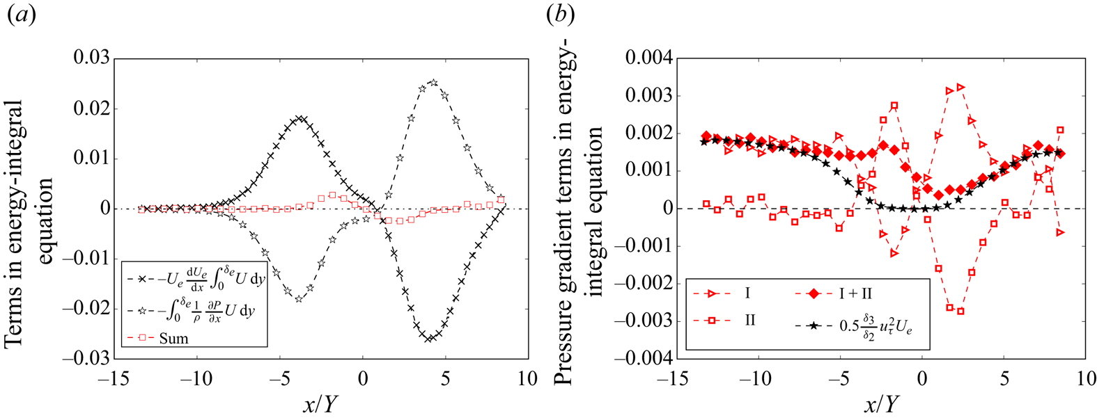
Many previous studies have assumed that  $\partial (P/\rho )/\partial x \approx -U_e\,{\rm d}U_e/{\rm d}\kern0.07em x$. However, Wei et al. (Reference Wei, Li and Wang2024) have shown that this assumption is valid only for weak pressure gradients, becoming invalid under strong pressure gradients. Figure 16(a) illustrates the second component on the right-hand side of (B3) and the integral resulting from the pressure force multiplied by
 $U$. The figure indicates that both components are close to zero under weak pressure gradients. However, under strong pressure gradients, they differ, yet their sum is significantly smaller than either component alone. Moreover, the magnitude of the sum is comparable to terms
 $\mathrm {I}, \mathrm {III}, \mathrm {IV}, \mathrm {V}, \mathrm {VI}$ in (3.2). Therefore, the second component on the right-hand side of (B3) is combined with the integral arising from the pressure gradient to form term
 $\mathrm {II}$ in (3.2).
(a) Variation of  $-U_e\,({\rm d}U_e/{\rm d}\kern0.07em x) \int _0^{\delta _e} U\,{\rm d} y$,
 $-\int _0^{\delta _e} (1/\rho )(\partial P/\partial x)U\,{\rm d} y$, and sum. (b) Terms
 $\mathrm {I}$,
 $\mathrm {II}$ and sum, compared with the ZPG approximation equation. Data are from DNS of Coleman et al. (Reference Coleman, Rumsey and Spalart2018).

Figure 16(b) presents the terms  $\mathrm {I}$,
 $\mathrm {II}$, and their sum. Additionally, the approximation given by (2.3) is also included, demonstrating that the approximation equation aligns well with the sum of terms
 $\mathrm {I}$ and
 $\mathrm {II}$ in the region where the pressure gradients are small.