1. Introduction
(a) The disintegration of a liquid jet injected into a gas cross-flow obtained by shadowgraph technique (Eslamian, Amighi & Ashgriz Reference Eslamian, Amighi and Ashgriz2014); boxes (1) and (2) in (a) mark the locations of the surface and the column breakup, respectively. (b) Illustration of the boundary-layer stripping mechanism, with the dotted line marking the boundary-layer edge inside the jet. (c) Schematic side view of a liquid jet in cross-flow showing formation of azimuthal and axial instabilities on the jet surface. (d) Schematic view of a cross-section of the jet at a short distance above the injection point and the cylindrical coordinate used in the stability analysis.

The normal injection of a liquid jet into a gaseous flow (often referred to as ‘liquid jet in cross-flow’) has a number of important engineering applications, such as in combustion systems of gas turbines and jet engine augmenters. A perpendicular contact between the jet and the ambient gas flow maximizes the exchange of momentum between the two phases. This leads to rapid disintegration of the liquid jet and facilitates production of a liquid spray which is necessary for an efficient combustion process. The disintegration of the jet generally consists of two processes: (a) the ‘surface breakup’ process, which corresponds to the separation of ligaments and droplets from the jet surface; and (b) the ‘column breakup’, which refers to disintegration of the liquid column as a whole. Figure 1(a) shows a snapshot of a jet breakup, taken from experiments by Eslamian et al. (Reference Eslamian, Amighi and Ashgriz2014). Approximate regions of the two breakup processes are marked in this figure by boxes. The surface breakup begins close to the nozzle (from which the jet is injected) and extends upward (as shown by box (1)). The column breakup process, however, occurs at the region which is sufficiently away from the nozzle to allow for the growth of large-scale waves leading to the column breakup (shown by box (2)). The liquid fragments shedding from the jet along its trajectory undergo subsequent secondary breakup processes leading to smaller and smaller droplet sizes, and hence to the formation of a spray. Various experimental measurements of droplet size distribution at the downstream of the jet have demonstrated the existence of a dichotomy in size, which implies the occurrence of the two underlying distinctly different breakup processes (e.g. Inamura & Nagai Reference Inamura and Nagai1997; Wu et al. Reference Wu, Kirkendall, Fuller and Nejad1998; Lubarsky et al. Reference Lubarsky, Reichel, Zinn and McAmis2010). Most of the experimental observations have used the shadowgraph technique, which only provides a 2D view of the jet, such as that shown in figure 1(a). The figure only shows the windward surface and the jet column breakup process. Shadowgraph images do not provide much information on the surface breakup. It is practically difficult to investigate details of the surface breakup process using experiments due to the smallness of scales involved. Moreover, the dense spray existing in the vicinity of the jet surface obstructs observation of surface breakup. Some studies, however, have speculated that the surface breakup is related to the visible waves on the jet windward surface (e.g. Mazallon, Dai & Faeth Reference Mazallon, Dai and Faeth1999). Sallam, Aalburg & Faeth (Reference Sallam, Aalburg and Faeth2004) used holographic technique to obtain more information on the jet breakup at the near nozzle region. They observed that the liquid fragments appear mostly from the lateral sides of the jet. Recently, numerical simulations (Pai et al. Reference Pai, Bermejo-Moreno, Desjardins and Pitsch2009; Herrmann Reference Herrmann2010; Li et al. Reference Li, Arienti, Soteriou and Sussman2010; Xiao, Dianat & McGuirk Reference Xiao, Dianat and McGuirk2013) have been employed to gain a better understanding of the jet breakup phenomena. Nevertheless, the underlying physical mechanisms of the surface breakup remain an open question.
A commonly accepted mechanism for the surface breakup of a liquid jet is the ‘boundary-layer stripping’ mechanism, which is illustrated schematically in figure 1(b) for a cross-section of the jet. In this mechanism, a viscous boundary layer forms at the jet periphery due to the existing shear between the gas and the liquid phases. Eventually, liquid droplets are pinched-off of the boundary layer formed inside the jet due to the outer gas flow. The diameters of the droplets formed in this way are proportional to the thickness of the liquid boundary layer. This idealized breakup process has been previously employed in the context of breakup of individual liquid drops subject to shock waves (Ranger & Nicholls Reference Ranger and Nicholls1969; Hsiang & Faeth Reference Hsiang and Faeth1992; Chou, Hsiang & Faeth Reference Chou, Hsiang and Faeth1997), and the breakup of liquid–gas mixing layers (Wu, Ruff & Faeth Reference Wu, Ruff and Faeth1991). This model has led to the development of correlations for the size and formation rate of droplets produced from the surface breakup (Sallam et al. Reference Sallam, Aalburg and Faeth2004), which has been employed in simplified atomization models for a liquid jet in cross-flow (Madabhushi Reference Madabhushi2003; Khosla & Crocker Reference Khosla and Crocker2004; Mashayek, Behzad & Ashgriz Reference Mashayek, Behzad and Ashgriz2011). Several experimental and numerical studies have questioned the viscous interpretation of surface breakup in this method and supported an inviscid breakup mechanism (Liu & Reitz Reference Liu and Reitz1997; Han & Tryggvason Reference Han and Tryggvason2001).
We postulate that the surface breakup of a jet in cross-flow can be a result of hydrodynamic instabilities on the jet lateral surface. The gas cross-flow moving around the transverse jet is usually at much higher velocity than the horizontal velocity component of the jet. This significant relative velocity between the gas cross-flow and the liquid jet, as well as the discontinuity in their properties, may result in instabilities at the surface of the jet in the azimuthal direction. The growth of such azimuthal instabilities leads to the formation of interface corrugations (see figure 1(c)), which finally detach as liquid ligaments from the surface of the jet. Note that another form of instability develops on the jet windward surface farther away from the nozzle (shown in figure 1(a) and schematically in figure 1(c)). This axial instability, which is responsible for the column breakup, is greatly influenced by the jet deflection and deformation. In this study, we focus on the surface breakup process through azimuthal instabilities (i.e. the near-nozzle problem). Investigation of the column breakup process at the downstream of the nozzle requires a different theoretical framework (from hydrodynamic instability analysis perspective), which warrants a separate study. Moreover, our focus herein is on the disintegration of a ‘laminar’ liquid jet in a cross-flow. In other words, we consider the sole effect of gas aerodynamic forces on the breakup of the jet. Wu et al. (Reference Wu, Kirkendall, Fuller and Nejad1997) and Sallam et al. (Reference Sallam, Aalburg and Faeth2004) also used super-cavitating nozzles with sharp-edged inlets/exits and small length-to-diameter ratio to create a non-turbulent jet in their experiments. Thus, similar to their set-up, in this study the primary breakup of the jet is caused by the cross-flow rather than by jet turbulence (which could lead to other breakup processes such as turbulent primary breakup (see e.g. Lee et al. Reference Lee, Aalburg, Diez, Faeth and Sallam2007)).
Our goal is to theoretically investigate the existence and characteristics of the azimuthal instabilities in a jet in cross-flow. This will pave the way for future investigation on the influence of important flow parameters (such as the liquid-to-gas density ratio, viscosity ratio and the surface tension) on the breakup process and thereby on the size distribution in the resulting spray which is of practical importance insofar as the design of combustion systems is concerned.
Despite the lack of theoretical attempts on investigating the hydrodynamic instabilities existing in liquid jets in cross-flows, the instabilities of transverse jets exposed to cross-flows with identical densities have been more extensively studied in the literature (Kelso, Lim & Perry Reference Kelso, Lim and Perry1996; Yuan, Street & Ferziger Reference Yuan, Street and Ferziger1999; Lim, New & Luo Reference Lim, New and Luo2001; Marzouk & Ghoniem Reference Marzouk and Ghoniem2007; de B. Alves, Kelly & Karagozian Reference de B. Alves, Kelly and Karagozian2008). Various inter-related set of vortical structures including shear layers vortices and counter-rotating vortex pair have been recognized as the outcomes of hydrodynamic instabilities. Yuan et al. (Reference Yuan, Street and Ferziger1999) has speculated shear instabilities on the lateral edges of the jet as the dominant growing modes of instability, which lead to the formation of the so-called ‘hanging’ vortices at this region. Muppidi & Mahesh (Reference Muppidi and Mahesh2006) observed similar instabilities developed on the sides of a two-dimensional model of a jet in cross-flow. However, it remains to be investigated whether the same holds true for the case of liquid-in-gas configuration.
We perform a temporal linear stability analysis of the near-nozzle liquid jet in cross-flow, where the azimuthal instabilities emerge. The analysis is based on the one-fluid formulation of the two phases, in which the fluids properties vary smoothly but steeply across the interface. This approach has been commonly employed in numerical studies of two-phase flows. Our choice of one-fluid formulation, thus, allows for direct comparison with results from high-resolution numerical simulations. To apply stability analysis to the jet in cross-flow configuration, we also develop an approximate theoretical solution for the gas cross-flow and the liquid jet flow fields. The stability analyses reveal that shear instability (not necessarily of Rayleigh type (Rayleigh Reference Rayleigh1880)) as well as centrifugal Rayleigh–Taylor instability (Fung Reference Fung1983) are the two existing types of azimuthal instabilities, with the former dominating. The flow destabilization mechanisms in several liquid–gas configurations have been investigated previously. Experimental and theoretical studies on a liquid jet surrounded by a coaxial air flow (air-blast atomization) have introduced the shear instability as the primary and the Rayleigh–Taylor instability as the secondary destabilization mechanisms (e.g. Varga, Lasheras & Hopfinger Reference Varga, Lasheras and Hopfinger2003; Marmottant & Villermaux Reference Marmottant and Villermaux2004, and references therein). The breakup of liquid drops exposed to high-speed gas flows have been also discussed in the context of hydrodynamic instabilities (Joseph, Belanger & Beavers Reference Joseph, Belanger and Beavers1999; Theofanous et al. Reference Theofanous, Mitkin, Ng, Chang, Deng and Sushchikh2012; Girin Reference Girin2014). Recently, more advanced stability analyses have been exploited to understand other plausible modes of instability for two-phase parallel flows (e.g. Boeck & Zaleski Reference Boeck and Zaleski2005; Otto, Rossi & Boeck Reference Otto, Rossi and Boeck2013). In this study, we present a theoretical investigation on the instabilities of a jet in cross-flow set-up. Furthermore, the construction of theoretical solutions for flows in both phases distinguishes the current work from the available literature on shear instabilities which is based on the employment of idealized velocity and density profiles (such as linear, hyperbolic tangent). We also investigate the influence of liquid-to-gas density ratio, which is known to be a key parameter in setting size distribution in spray systems, on the stability characteristics. The analyses show that an increase in the density ratio may have both destabilizing and stabilizing effect on the shear instability. We demonstrate that such effects are indeed consistent with the recent findings of Behzad & Ashgriz (Reference Behzad and Ashgriz2014) (hereafter BA) on the role of density variation on the instability of two-phase parallel flows.
This paper is organized as follows. In § 2, the problem set-up and the governing equations are presented, following by an introduction on the linear stability analysis in § 3. In § 4, the approach used to calculate the background flow fields (in both phases) is explained briefly, while a comprehensive discussion on that is provided in appendix A. In § 5, we discuss the results of the analysis, and we close with final discussions and the most important implications of the results in § 6.
2. Problem formulation
The stability analysis of a liquid flow in a gaseous medium is usually carried out by employing two sets of governing equations, one for each phase, and applying kinematic and dynamic matching conditions at the interface. In this study, however, we only consider one set of governing equations for both phases by employing the continuum surface force (CSF) approach (Brackbill, Kothe & Zemach Reference Brackbill, Kothe and Zemach1992). In this one-fluid formulation, the surface tension is represented by a continuous source term in the governing equations. Furthermore, the fluid properties vary continuously but steeply across the interface between the two phases. A non-dissipative scalar function,
 ${\it\phi}$
(to be defined), is often introduced to track the interface and thereby facilitate the transition between the properties of the two phases across the interface. This methodology has been widely used in numerical simulations of immiscible two-phase flows to capture the interface dynamics (Sussman, Smereka & Osher Reference Sussman, Smereka and Osher1994; Chang et al.
Reference Chang, Hou, Merriman and Osher1996; Sussman et al.
Reference Sussman, Fatemi, Smereka and Osher1998; Olsson & Kreiss Reference Olsson and Kreiss2005).
The problem is set up in a cylindrical coordinate in which the
 $z$
-direction is aligned with the direction of injection of the liquid jet, and the jet cross-section is described by
 $r$
and
 ${\it\theta}$
coordinates as shown in figure 1(d). In this coordinate system, the non-dimensional incompressible Navier–Stokes equations, the continuity equation and the transport equation for the scalar function are
 $$\begin{eqnarray}\displaystyle & {\it\rho}\left(\displaystyle \frac{\partial \boldsymbol{u}}{\partial t}+\boldsymbol{u}\boldsymbol{\cdot }\boldsymbol{{\rm\nabla}}\boldsymbol{u}\right)=-\boldsymbol{{\rm\nabla}}p+\displaystyle \frac{1}{\mathit{Re}}\boldsymbol{{\rm\nabla}}\boldsymbol{\cdot }{\bf\tau}+\frac{1}{We}\boldsymbol{F}_{\boldsymbol{s}}, & \displaystyle\end{eqnarray}$$
 $$\begin{eqnarray}\displaystyle & \boldsymbol{{\rm\nabla}}\boldsymbol{\cdot }\boldsymbol{u}=0, & \displaystyle\end{eqnarray}$$
 $$\begin{eqnarray}\displaystyle & \displaystyle \frac{\partial {\it\phi}}{\partial t}+\boldsymbol{u}\boldsymbol{\cdot }\boldsymbol{{\rm\nabla}}{\it\phi}=0, & \displaystyle\end{eqnarray}$$
 $\boldsymbol{{\rm\nabla}}$
is the gradient operator in the cylindrical coordinate, and
 ${\bf\tau}={\it\mu}(\boldsymbol{{\rm\nabla}}\boldsymbol{u}+\boldsymbol{{\rm\nabla}}\boldsymbol{u}^{\text{T}})$
is the viscous stress tensor,
 $\boldsymbol{F}_{\boldsymbol{s}}$
represents the continuous surface tension force (to be discussed shortly) and
 $\boldsymbol{u}$
,
 $p$
,
 ${\it\rho}$
and
 ${\it\mu}$
represent the velocity, pressure, density and viscosity, respectively. The governing equations have been non-dimensionalized by the cross-flow free-stream velocity
 $U_{c}^{\ast }$
, the cross-flow density
 ${\it\rho}_{c}^{\ast }$
, its viscosity
 ${\it\mu}_{c}^{\ast }$
, and the jet exit radius
 $R^{\ast }$
, in which the asterisk denotes a dimensional quantity. The non-dimensional velocity components are denoted by
 $u,v$
and
 $w$
in the azimuthal (tangential)
 ${\it\theta}$
, radial
 $r$
and the axial
 $z$
directions, respectively (figure 1(c,d)). The dimensionless parameters
 $\mathit{Re}$
and
 $\mathit{We}$
are the Reynolds and Weber numbers defined as
 $\mathit{Re}={\it\rho}_{c}^{\ast }U_{c}^{\ast }R^{\ast }/{\it\mu}_{c}^{\ast }$
and
 $\mathit{We}={\it\rho}_{c}^{\ast }{U_{c}^{\ast }}^{2}R^{\ast }/{\it\sigma}$
, where
 ${\it\sigma}$
is the surface tension. Since the Froude number (defined as
 $U_{c}^{\ast }/\sqrt{gR^{\ast }}$
, where
 $g$
is gravitational acceleration) is very high in all applications for which this work might have implications, the gravity force is negligible in the analysis.
We define the scalar
 ${\it\phi}$
to be a signed distance function, referring to the shortest distance of point
 $x_{i}$
in the domain from the interface. This scalar function (commonly referred to as the ‘level set’ function) has negative values in the gas phase and positive values in the liquid phase (Sussman et al.
Reference Sussman, Fatemi, Smereka and Osher1998). The interface is, therefore, represented by zero level set contour, i.e.
 $\{x_{i}\mid {\it\phi}(x_{i},t)=0\}$
. The density and viscosity profiles on the entire domain are hence defined as
 $$\begin{eqnarray}{\it\rho}({\it\phi})=1+\left(\frac{{\it\rho}_{j}}{{\it\rho}_{c}}-1\right)H({\it\phi}),\quad {\it\mu}({\it\phi})=1+\left(\frac{{\it\mu}_{j}}{{\it\mu}_{c}}-1\right)H({\it\phi}),\end{eqnarray}$$
where subscripts
 $c$
and
 $j$
denote the cross-flow and the jet properties. Here
 $H({\it\phi})$
is a regularized Heaviside function defined as
 $H({\it\phi})=(1+\tanh ({\it\phi}/{\it\delta}_{d}))/2$
, in which
 ${\it\delta}_{d}$
is the length scale of variation of fluid properties across the interface. And, finally, using CSF approach allows one to represent the surface tension by a continuous force term on the right-hand side of (2.1a
), as
 $$\begin{eqnarray}\boldsymbol{F}_{\boldsymbol{s}}={\it\kappa}({\it\phi}){\it\delta}({\it\phi})\boldsymbol{{\rm\nabla}}{\it\phi},\end{eqnarray}$$
where
 ${\it\kappa}=-\boldsymbol{{\rm\nabla}}\boldsymbol{\cdot }(\boldsymbol{{\rm\nabla}}{\it\phi}/|\boldsymbol{{\rm\nabla}}{\it\phi}|)$
is the interface curvature, and
 ${\it\delta}({\it\phi})=\text{d}H/\text{d}{\it\phi}$
is a smoothed Dirac delta function.
3. Linear stability analysis
In this section, the details of the linear stability analysis, which is employed in § 5 to identify the azimuthal instabilities leading to surface breakup of the jet, is described. As mentioned in § 1, the focus on the surface breakup mechanism limits our attention to the near-nozzle region of the jet (right above the injection point at
 $z\lesssim 1$
) where the azimuthal instabilities begin to grow. For almost all practical applications of liquid jet injection into a gas cross-flow, the momentum flux ratio defined as the ratio of momentum flux of the jet to that of the cross-flow (i.e.
 $q={\it\rho}_{j}{U_{j}}^{2}/{\it\rho}_{c}U_{c}^{2}$
, where
 $U_{j}$
is the mean jet velocity) is relatively high (i.e.
 $q>10$
). Thus, the jet deflection (i.e. bending due to aerodynamic force) and deformation of the jet cross-section at this region is small and limited to surface disturbances (Wu et al.
Reference Wu, Kirkendall, Fuller and Nejad1997; Mashayek, Jafari & Ashgriz Reference Mashayek, Jafari and Ashgriz2008; Mashayek & Ashgriz Reference Mashayek and Ashgriz2009). The experimental observations in high
 $q$
and large gas Weber numbers have shown that at the onset of jet surface breakup near the nozzle, the ratio of the jet diameter to the jet exit diameter is
 ${\approx}1$
, implying negligible jet deformation at this region (see e.g. Sallam et al.
Reference Sallam, Aalburg and Faeth2004, and references therein). These near-nozzle characteristics of the jet at high momentum flux ratio can be leveraged to simplify the stability analysis by reducing the problem to a quasi-2D jet and thereby to allow for a theoretical progress. More specifically, we assume that the shear layer of the jet with a hypothetical cylindrical shape does not develop significantly in the vertical
 $z$
direction at regions close to the nozzle. Therefore, the flow field at the near-nozzle region may consist of the cross-flow 2D boundary layer around the jet in the (
 $r{-}{\it\theta}$
) plane, and the jet shear layer, which conveys the disturbances along its trajectory. With a frame of reference fixed to a
 $r$
–
 ${\it\theta}$
element of the jet, the disturbances can be considered to grow temporally. Thus, upon solving for the flow fields both inside the cylindrical jet and in the flow surrounding it, we can apply temporal linear stability analysis in the
 $r$
–
 ${\it\theta}$
plane to identify the azimuthal instabilities which grow on the jet lateral sides.
To begin the analysis, and following the classic normal mode analysis (Drazin & Reid Reference Drazin and Reid2004), the velocity, pressure and level set function are decomposed into a background component denoted by
 $\bar{(\cdot )}$
and infinitesimal disturbances denoted by
 $(\cdot )^{\prime }$
:
 $$\begin{eqnarray}u=\bar{u}(r,{\it\theta})+u^{\prime },\quad v=\bar{v}(r,{\it\theta})+v^{\prime },\quad p=\bar{p}(r,{\it\theta})+p^{\prime },\quad {\it\phi}=\bar{{\it\phi}}(r,{\it\theta})+{\it\phi}^{\prime }.\end{eqnarray}$$
The calculation of the background flow is postponed to the next section. Here, we make a number of additional assumptions. First, we note that in the viscous boundary layers which form adjacent to the interface, the tangential velocity component is much greater than the radial component:
 $\bar{v}\ll \bar{u}$
. This assumption is typical to all boundary-layer problems with large
 $\mathit{Re}$
numbers and is valid away from the stagnation point (or the leading edge in planar boundary-layer configurations). Both conditions apply to our case. Second, we make a key assumption in that the background velocity
 $\bar{u}$
varies in the azimuthal direction on a scale much larger than the wavelengths of azimuthal disturbances which grow on the interface. This assumption reduces the problem to a local stability analysis at a given
 ${\it\theta}_{\circ }$
and eliminates the complication of involving the azimuthal variations of the background flow in the stability analysis. Note, however, that the background flow varies from one position on the interface to another and therefore, the stability analysis applied to various azimuthal points on the interface yields different results. This enables us to investigate the variation in the growth rate and the wavelength of the instabilities as a function of the interface azimuthal location. This assumption (hereafter referred to as ‘local’ instability assumption) is subject to a posteriori verification: for any unstable wavenumber obtained from our analyses at an azimuthal location
 ${\it\theta}_{\circ }$
to be considered valid, its wavelength (
 $R{\it\lambda}$
) needs to be much smaller than the length scale of variation of
 $\bar{u}$
in the azimuthal direction at this point, i.e.
 $R{\it\lambda}\ll Ru/u_{{\it\theta}}$
. Based on the aforementioned assumptions, (3.1) reduces to
 $$\begin{eqnarray}u=\bar{u}(r;{\it\theta}_{\circ })+u^{\prime },\quad v=v^{\prime },\quad p=\bar{p}({\it\theta})+p^{\prime },\quad {\it\phi}=\bar{{\it\phi}}(r)+{\it\phi}^{\prime }.\end{eqnarray}$$
Furthermore, the background level set function is defined as
 $\bar{{\it\phi}}(r)=R-r$
, which satisfies the background transport equation as well. Hence, the corresponding background density,
 $\bar{{\it\rho}}$
, and viscosity,
 $\bar{{\it\mu}}$
, profiles are both functions of
 $r$
alone.
Standard procedure resumes hereafter. First, a perturbation streamfunction is introduced which is related to the perturbation velocities through
 $$\begin{eqnarray}u^{\prime }=-\frac{\partial {\it\psi}^{\prime }}{\partial r}\quad \text{and}\quad v^{\prime }=\frac{1}{r}\frac{\partial {\it\psi}^{\prime }}{\partial {\it\theta}}.\end{eqnarray}$$
Next, the disturbances are expanded into normal (Fourier) modes through
 $$\begin{eqnarray}{\it\psi}^{\prime }=\hat{{\it\psi}}(r)\text{e}^{\text{i}(m{\it\theta}-{\it\omega}t)}\quad \text{and}\quad {\it\phi}^{\prime }=\hat{{\it\phi}}(r)\text{e}^{\text{i}(m{\it\theta}-{\it\omega}t)},\end{eqnarray}$$
where the azimuthal wavenumber
 $m=2{\rm\pi}/{\it\lambda}$
is real, and the frequency
 ${\it\omega}$
is complex with
 ${\it\omega}_{i}=\text{Im}({\it\omega})$
representing the growth rate and
 $c_{r}=\text{Re}({\it\omega})/m$
representing the angular phase speed (hereafter referred to as phase speed only for convenience). By substituting (3.4) into the governing equations (2.1), subtracting the background flow and linearizing the resulting perturbation equations, we arrive at the following pair of coupled equations for the perturbation functions
 $\hat{{\it\psi}}$
and
 $\hat{{\it\phi}}$
:
 $$\begin{eqnarray}\displaystyle & A_{1}+A_{2}+A_{3}=\displaystyle \frac{\text{i}}{\mathit{Re}}[A_{4}+A_{5}+A_{6}]+\displaystyle \frac{1}{\mathit{We}}[A_{7}], & \displaystyle\end{eqnarray}$$
 $$\begin{eqnarray}\displaystyle & A_{8}=0, & \displaystyle\end{eqnarray}$$
 $\text{i}=\sqrt{-1}$
. The
 $A_{i}$
terms are defined as
 $$\begin{eqnarray}\left.\begin{array}{@{}rcl@{}}A_{1}\, & =\, & \bar{{\it\rho}}\left[\left(\displaystyle \frac{{\it\omega}}{m}-{\it\Omega}\right)\left(\displaystyle \frac{m^{2}}{r}\hat{{\it\psi}}-\hat{{\it\psi}}_{r}-r\hat{{\it\psi}}_{rr}\right)-\bar{{\it\xi}}_{r}\hat{{\it\psi}}\right],\\ A_{2}\, & =\, & -\bar{{\it\rho}}_{r}\left[r\left(\displaystyle \frac{{\it\omega}}{m}-{\it\Omega}\right)\hat{{\it\psi}}_{r}+\bar{{\it\xi}}\hat{{\it\psi}}\right],\quad A_{3}=\bar{{\it\rho}}_{r}[r{\it\Omega}^{2}\hat{{\it\phi}}],\\ A_{4}\, & =\, & \bar{{\it\mu}}\left[\displaystyle \frac{m^{3}}{r^{3}}\left(\displaystyle \frac{4}{m^{2}}-1\right)\hat{{\it\psi}}-\left(2+\displaystyle \frac{1}{m^{2}}\right)\displaystyle \frac{m}{r^{2}}\hat{{\it\psi}}_{r}\right.\\ \, & \, & \left.+\,\displaystyle \frac{m}{r}\left(2+\displaystyle \frac{1}{m^{2}}\right)\hat{{\it\psi}}_{rr}-\displaystyle \frac{2}{m}\hat{{\it\psi}}_{rrr}-\displaystyle \frac{r}{m}\hat{{\it\psi}}_{rrrr}\right],\\ A_{5}\, & =\, & \bar{{\it\mu}}_{r}\left[-\displaystyle \frac{3m}{r^{2}}\hat{{\it\psi}}+\displaystyle \frac{m}{r}\hat{{\it\psi}}_{r}-\displaystyle \frac{1}{m}\hat{{\it\psi}}_{rr}-\displaystyle \frac{2r}{m}\hat{{\it\psi}}_{rrr}\right]-\bar{{\it\mu}}_{rr}\left[\displaystyle \frac{m}{r}\hat{{\it\psi}}-\displaystyle \frac{1}{m}\hat{{\it\psi}}_{r}+\displaystyle \frac{r}{m}\hat{{\it\psi}}_{rr}\right],\\ A_{6}\, & =\, & \left[\bar{{\it\mu}}_{r}\left(\displaystyle \frac{3-m^{2}}{m}{\it\Omega}_{r}-\displaystyle \frac{2}{m}\bar{{\it\xi}}_{r}+\displaystyle \frac{r}{m}({\it\Omega}_{rr}-\bar{{\it\xi}}_{rr})\right)\right.\\ \, & \, & \left.+\,\bar{{\it\mu}}_{rr}\left(\displaystyle \frac{r{\it\Omega}_{r}-2r\bar{{\it\xi}}_{r}}{m}\right)-\bar{{\it\mu}}_{rrr}\left(\displaystyle \frac{r^{2}{\it\Omega}_{r}}{m}\right)\right]\hat{{\it\phi}}\\ \, & \, & +\,\left[\bar{{\it\mu}}_{r}\left(\displaystyle \frac{r{\it\Omega}_{r}-2r\bar{{\it\xi}}_{r}}{m}\right)-2\bar{{\it\mu}}_{rr}\left(\displaystyle \frac{r^{2}{\it\Omega}_{r}}{m}\right)\right]\hat{{\it\phi}}_{r}-\left[\bar{{\it\mu}}_{r}\left(\displaystyle \frac{r^{2}{\it\Omega}_{r}}{m}\right)\right]\hat{{\it\phi}}_{rr},\\ A_{7}\, & =\, & \left[{\it\delta}(\bar{{\it\phi}})\left(\displaystyle \frac{1}{r^{2}}-\displaystyle \frac{m^{2}}{r^{2}}\right)\right]\hat{{\it\phi}},\\ A_{8}\, & =\, & r\left(\displaystyle \frac{{\it\omega}}{m}-{\it\Omega}\right)\hat{{\it\phi}}+\hat{{\it\psi}},\quad \end{array}\!\right\}\end{eqnarray}$$
where
 $r$
subscripts denote derivatives, and
 ${\it\Omega}=\bar{u}/r$
and
 $\bar{{\it\xi}}=\bar{u}_{r}+\bar{u}/r$
are the angular velocity and vorticity associated with the background flow, respectively. It is important to note that the terms
 $A_{2}$
and
 $A_{3}$
in (3.5a
) exist due to the radial variations in density while
 $A_{5}$
and
 $A_{6}$
exist due to the radial variations in viscosity. All four of these terms would be absent in a discontinuous formulation of the problem, in which two separate phases with a sharp interface are considered. However, in such cases, additional matching conditions at the discontinuities within the flow would need to be considered. For instance,
 $A_{2}$
in the present formulation corresponds to the dynamic matching condition in the sharp interface formulation, which is imposed at locations where vorticity or density jumps exist in the flow (commonly referred to as vorticity or density interface, respectively). As we will discuss in detail in the following sections, these terms can have important influences on the type and characteristics of the unstable modes.
Equations (3.5a
,
b
) form two coupled generalized eigenvalue problems with
 $\hat{{\it\psi}}$
and
 $\hat{{\it\phi}}$
as the eigenfunctions and
 ${\it\omega}$
as the eigenvalue. To solve this system, proper boundary conditions need to be applied. For that, it is required that the perturbations in the cross-flow field decay as
 $r\rightarrow \infty$
and the perturbations in the jet decay towards the centre of the jet (i.e. as
 $r\rightarrow 0$
). Since the viscosity and surface tension forces continuously vary across the interface, there is no need for explicitly imposing the kinematic and dynamic matching conditions at the interface. We solve the coupled system numerically by employing a second-order-accurate finite difference discretization in the radial direction with variable grid size. The outer boundary of the computational domain is taken to be sufficiently far from the jet to have no influence on the properties of the unstable modes. Upon discretization of the domain, the coupled system takes the following matrix form:
 $$\begin{eqnarray}\left[\begin{array}{@{}cc@{}}\unicode[STIX]{x1D61F}_{11} & \unicode[STIX]{x1D61F}_{12}\\ \unicode[STIX]{x1D61F}_{21} & \unicode[STIX]{x1D61F}_{22}\end{array}\right]\left[\begin{array}{@{}c@{}}\hat{{\it\psi}}\\ \hat{{\it\phi}}\end{array}\right]={\it\omega}\left[\begin{array}{@{}cc@{}}\unicode[STIX]{x1D620}_{11} & \unicode[STIX]{x1D620}_{12}\\ \unicode[STIX]{x1D620}_{21} & \unicode[STIX]{x1D620}_{22}\end{array}\right]\left[\begin{array}{@{}c@{}}\hat{{\it\psi}}\\ \hat{{\it\phi}}\end{array}\right],\end{eqnarray}$$
where
 $\unicode[STIX]{x1D61F}_{ii}$
and
 $\unicode[STIX]{x1D620}_{ii}$
are the coefficient matrices consisting of the background flow information and the wavenumber:
 $$\begin{eqnarray}\unicode[STIX]{x1D61F}_{ii},\unicode[STIX]{x1D620}_{ii}\equiv f(m,\mathit{Re},\mathit{We},,\bar{u},\bar{u}_{r},\bar{u}_{rr},\bar{u}_{rrr},\bar{{\it\rho}},\bar{{\it\rho}}_{r},\bar{{\it\mu}},\bar{{\it\mu}}_{r},\bar{{\it\mu}}_{rr},\bar{{\it\mu}}_{rrr}).\end{eqnarray}$$
The background flow velocity and its derivatives, the calculation of which will be described in the next section, are considered as a priori known parameters in the stability analysis.
At this stage, it is insightful to make connections between the current formulation and earlier works in the context of hydrodynamic stability analysis. By replacing the level set scalar with temperature and allowing
 $r\rightarrow \infty$
and
 $m\rightarrow \infty$
, such that
 $k=m/r$
remains finite, equation (3.5a
) reduces to the thermal Orr–Sommerfeld equation derived by Wall & Wilson (Reference Wall and Wilson1996) for the stability analysis of channel flows with temperature-dependent viscosity, where
 $k$
is the planar wavenumber. If it is further assumed that
 $\bar{{\it\rho}}$
and
 $\bar{{\it\mu}}$
are constants, then the classic Orr–Sommerfeld equation is recovered. Moreover, considering (3.5) in the limit of infinite Reynolds and Weber and numbers, the instability equation of a radially stratified vortex subject to a non-axisymmetric (azimuthal) perturbation is obtained (Fung Reference Fung1983, Reference Fung1986). This equation is analogous to the Taylor–Goldstein equation for planar flow with the distinction that term
 $A_{3}$
(which represents the centrifugal acceleration) provides the substitute for the buoyancy term. In such limit, a criterion can be determined for the azimuthal stability as follows: first we use (3.5b
) to rewrite
 $\hat{{\it\phi}}$
in terms of
 $\hat{{\it\psi}}$
in (3.5a
), then we rewrite (3.5a
) in terms of a new variable
 $\hat{{\it\chi}}\equiv \hat{{\it\psi}}/\sqrt{(\bar{u}/r-c)}$
. Upon multiplying the transformed (3.5a
) by the conjugate of
 $\hat{{\it\chi}}$
and integrating over the domain in
 $r$
, and after some mathematical manipulations, the imaginary part of the equation gives
 $$\begin{eqnarray}c_{i}\int \left[r\bar{{\it\rho}}\Vert \hat{{\it\chi}}_{r}\Vert ^{2}+\frac{m^{2}}{r}\bar{{\it\rho}}\Vert \hat{{\it\chi}}\Vert ^{2}\right]\,\text{d}r=c_{i}\int \left[\left(\frac{\bar{{\it\rho}}(\bar{u}_{r}-\bar{u}/r)^{2}}{4r}-\bar{{\it\rho}}_{r}\left(\frac{\bar{u}}{r}\right)^{2}\right)\frac{\Vert \hat{{\it\chi}}\Vert ^{2}}{\Vert \bar{u}/r-c\Vert ^{2}}\right]\,\text{d}r,\end{eqnarray}$$
where
 $c_{i}={\it\omega}_{i}/m$
is the scaled growth rate. Since the integral on the left-hand side is positive definite, existence of non-zero
 $c_{i}$
is only possible if the right-hand side integral is positive as well. Thus, linear stability of the jet with respect to azimuthal disturbances is guaranteed if
 $$\begin{eqnarray}\mathit{Ri}(r)\equiv \frac{\bar{{\it\rho}}_{r}}{\bar{{\it\rho}}}\frac{\bar{u}^{2}/r}{(\bar{u}_{r}-\bar{u}/r)^{2}}\geqslant 1/4\end{eqnarray}$$
everywhere within the flow. The Richardson number defined in (3.10) is analogous to that defined in the context of stratified shear layers in the presence of gravity. In the current study, however, the role of gravitational acceleration is replaced by the centrifugal acceleration. It should be noted that criterion (3.10) is only achievable if the jet density is lower than the cross-flow density. Therefore, for the purposes of the current work, which correspond to a dense jet injected into a lighter medium, the jet periphery will always be potentially unstable to the centrifugal Rayleigh–Taylor (CRT) type of azimuthal instability. Studies on the stability of vortices in which density decreases monotonically in the radial direction have demonstrated the possibility of the CRT instability (Fung Reference Fung1983; Sipp et al. Reference Sipp, Fabre, Michelin and Jacquin2005; Dixit & Govindarajan Reference Dixit and Govindarajan2011). This type of instability is analogues to the typical Rayleigh–Taylor instability; however, while the latter instability can exist without flow inertia, the CRT instability owes its existence to the rotational motion of the mean flow.
4. Background flow velocity
In this section we provide a brief discussion on the theoretical calculation of the background flow
 $\bar{u}$
which is required for the stability analysis discussed in the previous section. In the extensive literature on the linear stability analysis of shear flows in different contexts, most often the flows are assumed to be infinite or semi-infinite in the direction of the background shear. The background velocity, density and viscosity profiles are also frequently taken to be independent of one another and prescribed in form of idealized profiles (such as piecewise linear,
 $\tanh$
, erf, etc.). In the jet in cross-flow set-up, however, none of such simplifying assumptions can be made due to the complexity of the flow field around and inside the liquid jet. Most importantly, the gas flow around the liquid jet evolves from zero at the stagnation point (
 ${\it\theta}=180^{\circ }$
) on the windward surface of the jet to a fully developed boundary layer at the sides of the jet (
 ${\it\theta}=90^{\circ },270^{\circ }$
). In this section we discuss an approximate theoretical solution for the gas as well as liquid boundary layers which evolve on either side of the interface in the near nozzle region. The mathematical details are described comprehensively in appendix A. In the next section, we employ this solution in the aforementioned linear stability analyses to identify unstable modes on the windward side of the jet.
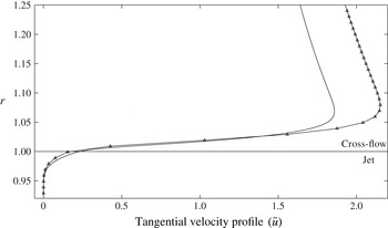
To begin, we emphasize that for cases with high jet-to-cross-flow momentum flux ratios, which are of primary concern in this study, the liquid jet deflects negligibly and preserves its nearly cylindrical shape in the near-nozzle region of interest. Therefore, the potential solution of flow around a solid cylinder can be employed as the background flow field for the flow around a liquid jet. However, this solution has a velocity jump at the liquid–gas interface from a high gas velocity in the cross-flow to zero liquid velocity in the jet and hence, it is only accurate outside the boundary layers. In reality, the viscosity smooths this sharp velocity gradient by forming boundary layers on either sides of the interface. Thus, an approximate viscous solution to the transverse jet flow field may be constructed by superposition of the potential flow component and a viscosity-induced component acting primarily in the vicinity of the interface. While the details of the calculation are included in the appendix A, here we include an example result. Figure 2 compares a background velocity profile obtained from a detailed numerical simulation of a liquid jet in cross-flow (Behzad, Ashgriz & Karney Reference Behzad, Ashgriz and Karney2014) with the one calculated based on the current approach under identical flow conditions of
 ${\it\rho}_{j}/{\it\rho}_{c}={\it\mu}_{j}/{\it\mu}_{c}=10$
and
 $\mathit{Re}=1200$
. Both profiles correspond to the sample point of
 $z_{\circ }=0.2$
and
 ${\it\theta}_{\circ }=90^{\circ }$
. The agreement is satisfactory.
Comparison of the calculated velocity profile (solid line) with that obtained from the numerical simulation of a liquid jet in cross-flow (symbolled line) (Behzad et al.
Reference Behzad, Ashgriz and Karney2014) at
 $z_{\circ }=0.2$
and
 ${\it\theta}_{\circ }=90^{\circ }$
and for identical flow conditions;
 ${\it\rho}_{j}/{\it\rho}_{c}={\it\mu}_{j}/{\it\mu}_{c}=10$
,
 $\mathit{Re}=1200$
,
 ${\it\delta}_{d}=0.005$
.

With a solution of background velocity at hand, we may now examine the local instability assumption discussed in § 3 for the background flow velocity. An estimate for the length scale associated with the background flow variation,
 $l_{b}$
, can be obtained as
 $l_{b}\sim |R\bar{u}_{\infty }/(\partial \bar{u}_{\infty }/\partial {\it\theta})|=|R\tan ({\it\theta})|$
, where
 $\bar{u}_{\infty }$
is the background velocity at far field (i.e.
 $r\rightarrow \infty$
) in the gas, determined in appendix A. Therefore, only unstable modes with wavenumbers higher than
 $2{\rm\pi}/({\it\epsilon}|\tan ({\it\theta}_{\circ })|)$
can satisfy the local instability assumption for
 ${\it\theta}={\it\theta}_{\circ }$
. As an example for the case with
 ${\it\theta}_{\circ }=100^{\circ }$
(see figure 3) and
 ${\it\epsilon}=0.2$
, the acceptable range of wavenumbers is
 $m>6$
. It should be noted that the wavenumber should be
 $m\geqslant 4$
, at any azimuthal location, to have physically meaningful results, for the current analysis in cylindrical coordinate.
5. Results and discussion
In this section, the results of the linear stability analysis are reported. The eigenvalue (3.5) in general can be applicable to a wide range of flow parameters. For practical reasons, however, we only consider a specific range of flow parameters in the current study. The experimental studies on the jet atomization have shown that the surface breakup is the dominant breakup process in the range of
 $\mathit{We}>60$
(Mazallon et al.
Reference Mazallon, Dai and Faeth1999; Sallam et al.
Reference Sallam, Aalburg and Faeth2004). Therefore, we fix the cross-flow Weber number at a relatively high value of
 $\mathit{We}=100$
to ensure we are in the correct regime. Since the jet and cross-flow properties are important in determining the appropriate strategy of injection in combustion systems, in this study, we are primarily concerned with investigating the jet-to-cross-flow density ratio effect on the flow stability. Although the effect of viscosity variation on the flow stability is also known to be important (see e.g. Yih Reference Yih1967; Ern, Charru & Luchini Reference Ern, Charru and Luchini2003), a uniform viscosity will be considered herein for both phases (i.e.
 ${\it\mu}_{j}/{\it\mu}_{c}=1$
). The analysis is performed on a jet cross-section located at
 $z_{\circ }=0.2$
, which is close enough to the nozzle so that the jet is not significantly deformed and, therefore, is consistent with the assumptions underlying the analysis. The results are shown to be almost insensitive to the precise location of the domain boundary in
 $r$
direction (defined as
 $(0,L)$
) when
 $L>2.5$
.
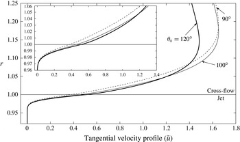
The background velocity profiles calculated for three different azimuthal locations;
 ${\it\rho}_{j}/{\it\rho}_{c}=25$
,
 $\mathit{Re}=100$
,
 ${\it\delta}_{d}=0.005$
.

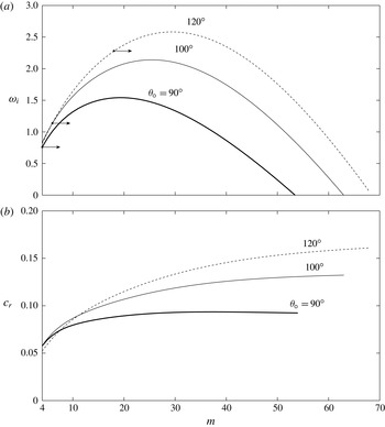
(a) The growth rate and (b) the phase speed of the unstable modes (
 $m\geqslant 4$
) at three azimuthal locations;
 ${\it\rho}_{j}/{\it\rho}_{c}=25$
,
 $\mathit{Re}=100$
,
 ${\it\delta}_{d}=0.005$
. The small arrows indicate the range of wavenumbers which satisfy the local instability assumption with
 ${\it\epsilon}=0.2$
.

Figure 3 shows three background velocity profiles calculated at
 ${\it\theta}_{\circ }=90^{\circ },100^{\circ }$
and
 $120^{\circ }$
for
 ${\it\rho}_{j}/{\it\rho}_{c}=25$
and
 $\mathit{Re}=100$
. At these locations, which are sufficiently far from the windward stagnation point, the variation of background velocity profile is negligible compared with the instability wavelength (to be verified shortly) and, therefore, the stability assumptions discussed in § 3 are less restrictive. Furthermore, experimental investigation of Sallam et al. (Reference Sallam, Aalburg and Faeth2004) has shown that the surface breakup initiates at the jet windward surface (i.e. over the segment of
 ${\it\theta}_{\circ }\in (90^{\circ },180^{\circ })$
prior to the flow separation in the leeward of the jet. Figure 4 compares the stability characteristics, the growth rate,
 ${\it\omega}_{i}$
, and the phase speed,
 $c_{r}$
, of the unstable modes for the three background velocity profiles shown in figure 3. Figure 4(a) shows bell-shaped growth rate curves (
 ${\it\omega}_{i}{-}m$
) similar to those obtained in stability analysis of inviscid shear flows. Although, we consider wavenumbers
 $m\geqslant 4$
in line with the geometry of the problem, the local instability assumption restricts the acceptable range of wavenumbers based on the azimuthal location. For
 ${\it\theta}_{\circ }=90^{\circ }$
, all wavenumbers satisfy this assumption while for all other
 ${\it\theta}_{\circ }$
, small arrows on the curves indicate the acceptable range of wavenumbers. At
 ${\it\theta}_{\circ }=90^{\circ }$
, the analysis predicts
 $m\approx 20$
for the fastest growing mode and
 $m\approx 54$
as the cut-off wavenumber (beyond that the flow is stable). By changing
 ${\it\theta}_{\circ }$
, the growth rate of the unstable modes changes, specifically in the high-wavenumber region. Figure 4(a) illustrates that as the background velocity profile develops in the azimuthal direction (from the windward stagnation point at
 ${\it\theta}_{\circ }=180^{\circ }$
to the side of the jet at
 ${\it\theta}_{\circ }=90^{\circ }$
), the instability progressively damps and the range of unstable modes shrinks. This variation is similar to a common feature of instabilities observed in shear layers. It was first stated by Rayleigh that a homogeneous inviscid parallel shear layer with a piecewise linear velocity profile is unstable to all disturbances whose wavelengths are larger than the order of vorticity thickness (as a length scale of the shear layer) (Rayleigh Reference Rayleigh1880). Similar scaling has been reported for the inviscid instability of two-phase parallel shear flows with piecewise linear velocity profiles (e.g. Lasheras & Hopfinger Reference Lasheras and Hopfinger2000). For such inviscid instabilities,
 $k_{c}{\it\delta}_{\bar{{\it\xi}}}$
(where
 $k_{c}$
is the planar cut-off wavenumber, and
 ${\it\delta}_{\bar{{\it\xi}}}$
is the vorticity thickness defined as
 ${\it\delta}_{\bar{{\it\xi}}}\equiv (\bar{u}_{max}-\bar{u}_{min})/\bar{{\it\xi}}_{max}$
) is a function of the background flow properties (i.e. density and viscosity ratios). In other words, the cut-off wavenumber is scaled by the vorticity thickness. Moreover, in this type of instability, the growth rate of the fastest growing mode is proportional to the difference between the free stream velocities in the two phases and inversely to the vorticity thickness, i.e.
 $\text{max}({\it\omega}_{i})\propto (\bar{u}_{max}-\bar{u}_{min})/{\it\delta}_{\bar{{\it\xi}}}$
. Therefore, a smaller vorticity thickness leads to a larger range of unstable mode and the amplification of instability in the flow. For the profiles shown in figure 3, the cross-flow vorticity thickness increases from
 ${\it\delta}_{\bar{{\it\xi}}}\approx 0.03$
to
 ${\it\delta}_{\bar{{\it\xi}}}\approx 0.055$
as
 ${\it\theta}$
decreases, leading to an analogous behaviour as observed in figure 4(a). The phase speed of the unstable modes is plotted in figure 4(b). As the figure shows, although the velocity in the cross-flow is higher than the velocity in the jet, the phase speed of the unstable modes is in the range of the velocity in the jet with an asymptotic limit in the high-wavenumber region. As discussed later, BA recently reported similar asymptotic behaviour for the phase speed of unstable modes corresponding to the inviscid instability of a parallel two-phase shear flow.
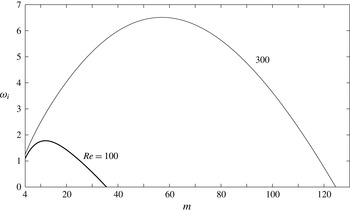
The growth rate of the unstable modes (
 $m\geqslant 4$
) for two Reynolds numbers of
 $\mathit{Re}=100$
(thick curve) and
 $\mathit{Re}=300$
(thin curve);
 ${\it\theta}_{\circ }=100^{\circ }$
,
 ${\it\rho}_{j}/{\it\rho}_{c}=25$
,
 ${\it\delta}_{d}=0.005$
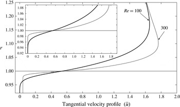
. The corresponding velocity profiles are plotted in figure 6.

The background velocity profiles calculated for two Reynolds numbers in figure 5.

The general effect of Reynolds number variation on the flow stability is shown in figure 5 for
 $\mathit{Re}=100$
and
 $\mathit{Re}=300$
corresponding to two different values of cross-flow viscosity
 ${\it\mu}_{c}^{\ast }$
(other variables in
 $\mathit{Re}$
remain fixed). The analyses are performed at
 ${\it\theta}_{\circ }=100^{\circ }$
and for
 ${\it\rho}_{j}/{\it\rho}_{c}=25$
, with the corresponding velocity profiles shown in figure 6. Figure 5 shows that the viscosity has a stabilization influence on the flow as documented previously (see e.g. Betchov & Szewczyk Reference Betchov and Szewczyk1963, and references therein). Both the range of the unstable modes and the growth rates are reduced as a result of decrease in Reynolds number. However, it should be pointed out that the influence of Reynolds number in the calculation of background velocity profiles can also intensify such effect. As figure 6 shows, the velocity profile calculated with higher
 $\mathit{Re}$
has a smaller vorticity thickness than that calculated with lower
 $\mathit{Re}$
. This results in a damping effect on the flow instability for decreasing Reynolds numbers due to scaling of stability characteristics with vorticity thickness (as discussed previously in terms of different azimuthal locations).
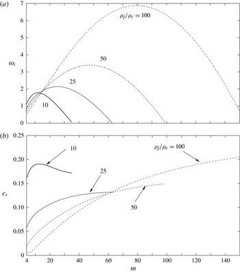
To investigate the effect of density ratio, the stability characteristics for several values of
 ${\it\rho}_{j}/{\it\rho}_{c}=10$
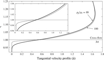
, 25, 50 and 100, are shown in figure 7. Figure 7(a) shows that a higher density ratio introduces a broader range of unstable modes. Figure 8 shows that the velocity profile with
 ${\it\rho}_{j}/{\it\rho}_{c}=100$
has smaller vorticity thicknesses (
 ${\it\delta}_{\bar{{\it\xi}}}\approx 0.029$
for the cross-flow and
 ${\it\delta}_{\bar{{\it\xi}}}\approx 0.008$
for the jet) compared with
 ${\it\rho}_{j}/{\it\rho}_{c}=10$
(
 ${\it\delta}_{\bar{{\it\xi}}}\approx 0.063$
for the cross-flow and
 ${\it\delta}_{\bar{{\it\xi}}}\approx 0.024$
for the jet). This results in a wider band of unstable wavenumbers and higher growth rates as the density ratio increases. Such behaviour is due to the scaling of these stability characteristics with the vorticity thickness as described previously. In the limit of
 ${\it\rho}_{j}/{\it\rho}_{c}\rightarrow \infty$
(zero vorticity thickness) and
 $\mathit{We}\rightarrow \infty$
, the flow is expected to be unconditionally unstable to ‘Kelvin–Helmholtz’ instability in the absence of surface tension (Drazin & Reid Reference Drazin and Reid2004). The influence of the jet with higher density ratio is also manifested in the reduction of the phase speed; however, this reduction is not significant for higher density ratios. Similar response was reported in BA as explained at the end of this section. Note that for any density ratio, the phase speeds are still within the range of maximum (
 ${\approx}1.6$
as in figure 8) and minimum (
 ${\approx}\,0.0$
) angular background velocity in the flow.
(a) The growth rate and (b) the corresponding phase speed of the unstable modes for various density ratios;
 ${\it\theta}_{\circ }=100^{\circ }$
,
 $\mathit{Re}=100$
,
 ${\it\delta}_{d}=0.005$
. Note that at this azimuthal location, the wavenumbers with
 $m>6$
satisfy the local instability assumption.

Despite the preceding destabilizing effect of increasing density ratios, there exists a narrow band in the low-wavenumber region in figure 7(a), in which an increase in density ratio stabilizes the flow. We suspect that this stabilizing influence is due to the dependence of the velocity profile to the density ratio. To examine this, the problem is simplified one step by decoupling the velocity profile from the density profile. In other words, we investigate different density profiles (corresponding to different density ratios) while keeping the background velocity profile fixed. With this simplification, one can explore the sole effect of density variation on the flow stability. For further simplicity (and without loss of generality), a hyperbolic tangent velocity profile of the form
 $\bar{u}=\tanh (y/{\it\delta}_{\bar{u}})/2$
is employed. Parameter
 $\mathit{Ri}_{\circ }\equiv \mathit{Ri}(r=1)=-\mathit{At}~{{\it\delta}_{\bar{u}}}^{2}/[{\it\delta}_{d}(1-{\it\delta}_{\bar{u}})^{2}]$
(where
 $\mathit{At}\equiv ({\it\rho}_{j}-{\it\rho}_{c})/({\it\rho}_{j}+{\it\rho}_{c})$
is the Atwood number) is also defined as an overall measure of density variation. This definition is similar to the bulk Richardson number commonly defined in stratified shear flows under buoyancy effect, except that in the current case the centrifugal acceleration substitutes the gravitational acceleration. For
 $\mathit{Ri}_{\circ }>0$
(corresponding to
 ${\it\rho}_{j}/{\it\rho}_{c}<1$
), the stratification is stable with regards to CRT instability. However, in the range of
 $\mathit{Ri}_{\circ }<0$
(corresponding to
 ${\it\rho}_{j}/{\it\rho}_{c}>1$
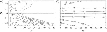
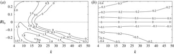
), the CRT instability coexists with shear instabilities. Figure 9 shows the contours of constant growth rate and the phase speed as a function of
 $\mathit{Ri}_{\circ }$
and
 $m$
, for the fixed parameters
 $\mathit{We}=\infty$
,
 $\mathit{Re}=1200$
,
 ${\it\delta}_{\bar{u}}=0.05$
and
 ${\it\delta}_{d}=0.005$
(note that
 ${\it\delta}_{d}$
smaller than 0.01 does not change the results). As figure 9(a) shows, for a liquid jet subjected to a gas cross-flow (
 $Ri_{\circ }<0$
), the density ratio has a non-monotonic effect. The increasing density ratios have a pure destabilizing effect in high-wavenumber band (
 $m>30$
). However, in the low-wavenumber band (
 $m<30$
), there is a dual effect of both destabilization and stabilization of density variation. For instance, for
 $m=10$
, increasing the density ratio from
 ${\it\rho}_{j}/{\it\rho}_{c}=1$
(
 $\mathit{Ri}_{\circ }=0$
) to
 ${\it\rho}_{j}/{\it\rho}_{c}=5$
(
 $\mathit{Ri}_{\circ }\approx -0.18$
) is destabilizing; however, further increasing of density ratio to
 ${\it\rho}_{j}/{\it\rho}_{c}=1000$
(
 $\mathit{Ri}_{\circ }\approx -0.27$
) progressively damps the instability. On the other hand, the region
 $\mathit{Ri}_{\circ }>0$
in figure 9(a) is analogous to the instability of statically stable stratified shear flows in low-Froude-number limit (Hazel Reference Hazel1972; Caulfield Reference Caulfield1994). In this region, a similar dual effect of density variation is noticed for wavenumbers approximately
 $m>10$
; nevertheless, a pure stabilizing effect of high density ratios can be observed for smaller wavenumbers.
The background velocity profiles calculated for two different densities corresponding to figure 7;
 ${\it\theta}_{\circ }=100^{\circ }$
,
 $\mathit{Re}=100$
,
 ${\it\delta}_{d}=0.005$
.

(a) The contours of constant growth rate and (b) the phase speed for a shear layer with a hyperbolic tangent velocity profile in cylindrical configuration;
 $\mathit{Re}=1200$
,
 $\mathit{We}=\infty$
,
 ${\it\delta}_{\bar{u}}=0.05$
,
 ${\it\delta}_{d}=0.005$
.

Thus, despite the density–velocity decoupling, we still observe a destabilization/stabilization influence due to the density itself. Now, we need to discuss reasons behind such isolated influence of the density ratio change. As discussed in § 3, application of a steeply varying continuous density profile, as opposed to a discontinuous profile, introduces two additional terms in the eigenvalue equations (3.5): (I) term
 $A_{2}$
representing the effect of density variation on the flow inertia; and (II) term
 $A_{3}$
which represents the radial acceleration associated with density perturbation. For
 $\mathit{Ri}_{\circ }<0$
,
 $A_{3}$
is responsible for the CRT instability, which is known to be amplified by increasing of the density ratio (see e.g. Dixit & Govindarajan Reference Dixit and Govindarajan2011, and references therein). Therefore, for increasing density ratios, one might speculate that the destabilizing density effect in CRT instability generates a non-monotonic behaviour of density variation as illustrated in figure 9(a). However, for a counterpart stability analysis in the planar configuration,
 $A_{3}$
vanishes and only
 $A_{2}$
remains. For this configuration, the growth rate and the phase speed contours with parameters identical to the cylindrical configuration are plotted in figure 10, in the
 $\mathit{Ri}_{\circ }{-}k$
space (note that in the planar configuration,
 $\mathit{Ri}_{\circ }$
is not a relevant parameter, however, it is applied here for the sake of comparison with the cylindrical configuration). Although the CRT term is absent in figure 10(a), it shows a very similar pattern of density variation effect as in the cylindrical case. Therefore, our earlier speculation about the influence of CRT instability on the behaviour of density variation does not hold true. In fact, comparison of figures 9 and 10 reveals no significant distinction between the two configurations, suggesting a minor influence of the CRT instability. Despite such finding, the question of influence of density variation on the flow stability remains unresolved. Hence, it is yet to be determined whether the employment of a continuous density formulation in the current stability problem is responsible for the stabilization/destabilization effect of density variation.
(a) The contours of constant growth rate and (b) the phase speed for a shear layer with a hyperbolic tangent velocity profile in planar configuration with the same flow parameters as in figure 9.

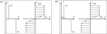
(a) The piecewise linear velocity profile with density discontinuity employed in BA. (b) The hyperbolic tangent velocity profile with continuous density profile used in the current study.

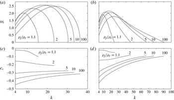
The effect of density ratio on the growth rate (a,b) and the corresponding phase speed (c,d) of the unstable modes for the piecewise linear velocity profile with the sharp interface (a,c) and for the hyperbolic tangent velocity profile with the smooth interface (b,d), under the identical flow parameters and in the planar configuration;
 $\mathit{Re}=\mathit{We}=\infty$
,
 ${\it\delta}_{\bar{u}}=0.05$
,
 ${\it\delta}_{d}=0.005$
. The corresponding configurations are schematically illustrated in figure 11.

BA examined the influence of density variation on the inviscid instability mechanism of a piecewise linear velocity profile (figure 11
a) with a density jump. They have demonstrated that the instability in such linear configuration is driven by a resonance between a neutrally stable wave due to the density interface (
 $y=0$
in figure 11
a) and vorticity waves (commonly referred to as Rayleigh waves) formed at the vorticity interfaces (
 $y=\pm {\it\delta}_{u}$
in figure 11
a). They also showed that an increase in the density ratio leads to extending of the range of unstable modes and introduces a destabilization/stabilization effect similar to the one observed in the present study. Figure 12 compares the effect of density ratios on the stability characteristics of a piecewise linear velocity profile in BA (figure 11
a) with those obtained for a hyperbolic tangent velocity profile in the present study (figure 11
b) under identical flow conditions and a planar configuration. Although in the current study both the background density and vorticity distribution continuously vary across the domain, figure 12 shows almost identical sensitivity to density variation in both set-ups. In this figure, a stabilizing effect of density in low-wavenumber region gradually changes to a destabilizing effect in high-wavenumber region. It is worth mentioning that in the sharp interface configuration of two-phase parallel flows (such as that of BA), the density discontinuity effect is considered in the dynamic matching condition at the density interface. In our continuous representation of the problem, however, the effect of density gradient on the inertial terms is considered explicitly in the momentum equation via term
 $A_{2}$
and
 $A_{3}$
of equation (3.5a
) throughout the flow. Nevertheless, figure 12 suggests that for sufficiently small length scale of density variation,
 ${\it\delta}_{d}$
(i.e. a relatively steep transition of density compared with that of velocity as in the present study), both approaches agree well in terms of the response of stability characteristics to the density variation. BA showed that the stabilizing/destabilizing response of density is mainly due to the resonating wave at the density interface whose phase speed is a function of density ratio. However, beyond density ratio
 ${\approx}100$
, no significant change was observed in the wave phase speed. In this work, we find a similar effect for the instability of a smoothly varying velocity and the corresponding density profiles. Thus, going back to the realistic flow configuration in figure 7(a), it can be concluded that the stabilization effect of density in low-wavenumber region of this figure is mainly due to the term
 $A_{2}$
, which considers the effect of density variation on the flow inertia. Furthermore, in the high wavenumbers, the destabilization due to the employment of density-dependence velocity profiles (employed in preparation of figure 7) predominates the sole destabilizing effect of term
 $A_{2}$
in this range.
As shown in figures 9(b) and 10(b) for a hyperbolic tangent velocity profile, the effect of density variation on the phase speed of the unstable modes is almost identical for both cylindrical and planar configurations. For the homogeneous planar shear flow with a symmetric background velocity profile (corresponding to
 $At=0$
in figure 10
b), counter-propagating neutral Rayleigh waves, on either sides of the interface, resonate and generate an unstable wave (Holmboe Reference Holmboe1962; Caulfield Reference Caulfield1994). This wave travels with a phase speed equal to the average background velocity, which is zero for the hyperbolic tangent profile (see figure 10
b). However, for a homogenous cylindrical shear flow (corresponding to
 $At=0$
in figure 9
b), the unstable wave travels with non-zero phase speeds (i.e.
 $c_{r}\neq 0$
). This is due to the asymmetry in the cylindrical configuration introduced by the curvature in problem geometry. In this configuration, the background vorticity profile is no longer symmetric, which produces Rayleigh waves with different phase speeds on either sides of the interface. Asymmetric Rayleigh waves, therefore, produce an unstable oscillatory wave, which travels with a non-zero phase speed. The effect of asymmetry in flow configuration was first documented by Hazel (Reference Hazel1972). He showed that slight changes in the fluid properties and/or the background velocity profile can noticeably alter the stability characteristics, specifically the phase speed.
For
 $\mathit{At}\neq 0$
, the phase speed of the unstable modes in both cylindrical and planar configurations (figures 9
b and 10
b, respectively) show that when the jet has a higher density than the cross-flow density (
 $\mathit{Ri}_{\circ }<0$
), the waves propagate in the negative direction (i.e. the direction of the higher density jet flow). Furthermore, increasing the density ratio leads to an increase in the phase speed of the unstable modes. BA also explained both of these effects for a symmetric piecewise linear velocity profile with a density jump (such as figure 11
a). They revealed that the neutral wave at the density interface propagates in the direction of the higher-density phase with a asymptotic phase speed which is monotonically increased by density ratio (see figure 12(c)). The continuous approach in the current study provides analogous results. For realistic conditions in figure 7(b), the unstable modes travel with phase speeds slower than the interface velocity (i.e. negative phase speeds with respect to the interface), showing the importance of density difference in the formation of unstable modes and setting the associated phase speeds.
6. Summary and conclusions
In this work we have presented a theoretical study of azimuthal instabilities which develop near the nozzle of a liquid jet injected normally into a gaseous cross-flow. We postulate that such instabilities may lead to the formation of interface corrugations and eventually to the jet surface breakup. Therefore, a temporal linear stability analysis was performed on the jet near the nozzle. One-fluid formulation of the governing equations was utilized analogous to the one commonly employed in the numerical methods of solving two-phase flows. Moreover, unlike the classic stability analysis in which the background velocity profile is known a posteriori, in this study a set of approximate governing equations were developed and solved for both the jet and the cross-flow to obtain a realistic background flow. Therefore, the stability results can be compared directly with the results of numerical studies for identical bulk flow parameters. The approximate solution of the background velocity profile holds for the near-nozzle region as it mainly relies on the assumption of high jet-to-cross-flow momentum flux ratio. Under this assumption, which is a typical condition in most of the engineering applications, the jet at the near-nozzle region remains in its original cylindrical shape with no significant bending and deformation. This allows for simplification of the problem and thereby facilitates theoretical progress in performing a quasi-2D normal-mode analysis of the background flows. To reduce the parameter space, the analyses were also conducted under constrained flow conditions including a uniform viscosity and a fixed cross-flow Weber number of
 $\mathit{We}=100$
, for which the surface breakup has been observed both experimentally and numerically (Wu et al.
Reference Wu, Kirkendall, Fuller and Nejad1997; Pai et al.
Reference Pai, Bermejo-Moreno, Desjardins and Pitsch2009).
According to the results, we have identified the shear instability (not necessarily of Rayleigh type) as the main type of azimuthal instability which can trigger the surface breakup of a liquid jet in cross-flow. This instability mechanism has an inviscid origin as opposed to the boundary-layer stripping mechanism commonly assumed to be responsible for the surface breakup. In other words, while the stripping mechanism cannot explain any surface breakup for inviscid jets and cross-flows (due to the absence of boundary layers), shear instabilities exist in such configurations. Furthermore, the rotational motion of the cross-flow allows the existence of the CRT instability; however, the shear instability dominates the CRT. The results of the analyses at different azimuthal locations on the jet periphery revealed that the instability wavelengths increase along the jet periphery in azimuthal direction from the windward to the leeward side of the jet. With regard to the size of droplets formed due to the surface breakup, such a variation in the wavelength of instability implies the appearance of smaller droplets close to the windward stagnation point compared with those formed near the jet lateral sides. It should be noted, however, that formation of droplets by means of shear instabilities is most probably facilitated through a series of second- and high-order instabilities as is often the case with shear-induced turbulence transition (see e.g. Lasheras & Hopfinger (Reference Lasheras and Hopfinger2000), Marmottant & Villermaux (Reference Marmottant and Villermaux2004) and Mashayek & Peltier (Reference Mashayek and Peltier2012a ,Reference Mashayek and Peltier b ) for a discussion in a different context).
The effect of density variation on the stability results was also investigated. The variation of density ratio not only changed the stability characteristics explicitly, but also changed the background velocity profile. An increase in density ratio decreased the vorticity thickness of the velocity both in the cross-flow and the jet. This broadened the range of unstable modes and increased the growth rate of the most amplified mode. Thus, one may expect the formation of smaller droplets due to the surface breakup when a higher density jet is used.
It was also found that an increase in the density ratio may exhibit either a stabilization effect or destabilization depending on the wavenumber under consideration. Similar behaviour was reported for the inviscid analysis performed on a piecewise linear velocity profile with an embedded density discontinuity by BA. They have explained the stabilizing/destabilizing density effect in terms of the resonance of neutrally stable waves in the flow. Our analyses of the jet in cross-flow problem showed that despite the continuous approach adapted in the current study, the density variation effects on the stability characteristics are almost analogous to the counterpart effects in sharp interface approach of BA. Therefore, it can be concluded that the same wave resonances still exist for the smoothly varying profiles, provided that the thickness of transition layer at the interface is sufficiently small. However, identifying the individual neutral waves for a continuous velocity profiles (as in current study) is not as simple as in the piecewise linear velocity profiles with sharp interface (see Iga Reference Iga2013, for more details). This finding is particularly relevant for the diffuse interface method commonly used in numerical simulations of two-phase flow problems, in which any sharp interface is represented by a very thin transition layer.
Finally, we point out that the current study only considers the near-nozzle region of a ‘laminar’ jet where azimuthal instabilities emerge. Such instabilities grow into interface corrugations which later separate along the jet trajectory during the surface breakup process. The axial instabilities, which appear on the jet windward surface far from the nozzle and lead to the disintegration of the whole jet, are entirely different. Those were not included in the present study and need to be addressed in a separate theoretical framework.
Appendix A
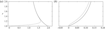
In this appendix the detailed theoretical calculation of background velocity profile discussed in § 4 is explained. The approach was previously made by Chao (Reference Chao1962) and Harper & Moore (Reference Harper and Moore1968) to calculate the flow field around and inside a nearly spherical liquid drop subject to a uniform gaseous flow with high Reynolds number. In their configuration, the potential flow solution has a continuous velocity at the interface. Therefore, they assumed that the flow field is only slightly disturbed from the irrotational flow solution past a liquid sphere, due to the existence of thin boundary layers. This assumption allowed them to linearize and thereby simplify the governing equations. For the jet in cross-flow, however, the potential flow solution is discontinuous and, therefore, the viscosity-induced velocity component tends to be the same order of the far-field gas velocity in order to satisfy the continuity of the velocity and the shear stress at the interface. This inhibits linearization of the momentum equation for the transverse jets as opposed to spherical drops. To remedy this, we adjust the potential solution of a flow past a cylinder such that it has zero tangential velocity at the interface similar to the jet flow. As discussed shortly, this ‘approximate flow field’ satisfies the continuity equation; however, it is not an exact solution of Navier–Stokes equations. Nevertheless, being superimposed by the viscosity-induced velocity component, which has now a relatively small value compared with the far-field velocity, it can provide a satisfactory approximation of the exact flow fields for the cross-flow and the jet (see figure 2).
We begin with adjustment of the potential solution for flow over a solid cylinder. Similar adjustment was previously employed by de B. Alves et al. (Reference de B. Alves, Kelly and Karagozian2008) in their stability analysis and adapted here for the current study. In this approach, the following hyperbolic tangent velocity profile (corresponding to profile No. 2 of Michalke (Reference Michalke1984) for free jets) is applied in order to remove the velocity discontinuity of potential flow across the interface:
 $$\begin{eqnarray}U_{o}(r)=\frac{1}{2}-\frac{1}{2}\tanh \left(\frac{1}{4Z_{o}}\left(r-\frac{1}{r}\right)\right),\end{eqnarray}$$
where the local non-dimensional parameter
 $Z_{o}$
depends on the distance above the jet injection in
 $z$
-direction and can be estimated as (Michalke Reference Michalke1984):
 $$\begin{eqnarray}Z_{o}=\frac{3z+4}{100}.\end{eqnarray}$$
The tangential velocity component of the approximate flow field for the cross-flow is, therefore, defined as follows:
 $$\begin{eqnarray}U(r,{\it\theta})=-\sin ({\it\theta})\left(1+\frac{1}{r^{2}}\right)(1-2U_{o}),\end{eqnarray}$$
which has zero value at the interface (
 $r=1$
) and approaches
 $-\sin ({\it\theta})$
as
 $r\rightarrow \infty$
similar to the potential flow over a solid cylinder (i.e.
 $-\sin ({\it\theta})(1+1/r^{2})$
). Using the corresponding continuity equation and a zero axial velocity component of the approximate flow field (i.e.
 $W=0$
) for the cross-flow, the radial velocity component can be obtained as
 $$\begin{eqnarray}V(r,{\it\theta})=\frac{4Z_{o}\cos ({\it\theta})}{r}\log \left(\cosh \left(\frac{1}{4Z_{o}}\left(r-\frac{1}{r}\right)\right)\right),\end{eqnarray}$$
which has zero value at the interface and approaches
 $\cos ({\it\theta})$
as
 $r\rightarrow \infty$
similar to the potential velocity component (i.e.
 $\cos ({\it\theta})(1-1/r^{2})$
).
de B. Alves et al. (Reference de B. Alves, Kelly and Karagozian2008) used almost similar approximate velocity profiles as the lowest-order solution of the background velocity in their stability analysis on a jet in cross-flow. They further added a next order to their solution of the background velocity profile. As discussed later, we add a viscosity-induced velocity component to these approximate velocity components
 $(U,V,W)$
to account for continuity of the velocities (cf. (A 10)) and the shear stress (cf. (A 11)) at the interface. Figure 13 shows the velocity components of the approximate representation and the potential flow solutions for flow past a solid cylinder (here a liquid jet with high momentum flux ratio).
The magnitude of tangential (a) and radial (b) velocity components corresponding to the potential (solid line) and the approximate flow field (dashed line) for flow over a liquid jet at
 $z_{\circ }=0.2$
and
 ${\it\theta}_{\circ }=80^{\circ }$
.

We now write the background velocity field
 $\bar{\boldsymbol{u}}=(\bar{u},\bar{v},\bar{w})$
and the pressure
 $\bar{p}$
within the boundary layers as follows:
 $$\begin{eqnarray}\bar{\boldsymbol{u}}=\boldsymbol{U}+\tilde{\boldsymbol{u}},\quad \bar{p}=P+\tilde{p},\end{eqnarray}$$
where
 $\boldsymbol{U}=(U,V,W)$
and
 $P$
are the approximate velocity field and the associated pressure and the viscosity-induced quantities are designated by
 $\tilde{(\cdot )}$
. After substituting (A 5) into the momentum and continuity equations and linearizing, we arrive at the following governing equations for the viscosity-induced variables:
 $$\begin{eqnarray}\displaystyle & \bar{{\it\rho}}(\tilde{\boldsymbol{u}}\boldsymbol{\cdot }\boldsymbol{{\rm\nabla}}\boldsymbol{U}+\boldsymbol{U}\boldsymbol{\cdot }\boldsymbol{{\rm\nabla}}\tilde{\boldsymbol{u}})=-\boldsymbol{{\rm\nabla}}\tilde{p}+\displaystyle \frac{1}{\mathit{Re}}\boldsymbol{{\rm\nabla}}\boldsymbol{\cdot }\tilde{{\bf\tau}}, & \displaystyle\end{eqnarray}$$
 $$\begin{eqnarray}\displaystyle & \boldsymbol{{\rm\nabla}}\boldsymbol{\cdot }\tilde{\boldsymbol{u}}=0, & \displaystyle\end{eqnarray}$$
 $U$
and
 $V$
in tangential and radial directions are defined by (A 3) and (A 4), respectively, and the axial velocity is
 $W=0$
. For the internal flow, however, the only approximate flow component is the jet mean velocity in the axial
 $z$
direction, i.e.
 $W=U_{j}$
and
 $U=V=0$
. Note that due to the difference in the approximate flow representation of the external and internal flows, we switch to a two-fluid formulation (with two sets of governing equations). However, it is still assumed that the density and viscosity continuously vary. We emphasize that such discontinuous formulation is only applied in calculation of background velocity profile; however, as described in § 2, a continuous form of governing equations is employed for stability analysis.
The velocity components induced by the viscosity in the boundary layers,
 $\tilde{\boldsymbol{u}}$
, are obtained by solving (A 6). Nevertheless, since we assume
 $\bar{u}\gg \bar{v}$
as one of the assumptions behind our stability analysis, we are only interested in the tangential (azimuthal) background velocity component. This component of (A 6a
) is
 $$\begin{eqnarray}\displaystyle & & \displaystyle \bar{{\it\rho}}\left(V\frac{\partial \tilde{u} }{\partial r}+\tilde{v}\frac{\partial U}{\partial r}+\frac{U}{r}\frac{\partial \tilde{u} }{\partial {\it\theta}}+\frac{\tilde{u} }{r}\frac{\partial U}{\partial {\it\theta}}+\frac{V\tilde{u} }{r}+\frac{U\tilde{v}}{r}+W\frac{\partial \tilde{u} }{\partial z}\right)\nonumber\\ \displaystyle & & \displaystyle \qquad =-\frac{1}{r}\frac{\partial \tilde{p}}{\partial {\it\theta}}+\frac{\bar{{\it\mu}}}{\mathit{Re}}\left({\rm\nabla}^{2}\tilde{u} -\frac{\tilde{u} }{r^{2}}+\frac{2}{r^{2}}\frac{\partial \tilde{v}}{\partial {\it\theta}}\right)+\frac{1}{\mathit{Re}}\frac{\text{d}\bar{{\it\mu}}}{\text{d}r}\left(-\frac{\tilde{u} }{r}+\frac{\partial \tilde{u} }{\partial r}+\frac{1}{r}\frac{\partial \tilde{v}}{\partial {\it\theta}}\right).\end{eqnarray}$$
Next, we apply an order of magnitude argument similar to that discussed by Chao (Reference Chao1962) to simplify (A 7). First, it is assumed that the boundary-layer thickness is thin, i.e.
 $\bar{{\it\delta}}\ll 1$
, where
 $\bar{{\it\delta}}$
is the average boundary-layer thickness. Second, the viscosity-induced quantities are small compared with the approximate velocities, i.e.
 $\tilde{u} \sim \tilde{w}\sim \mathit{O}({\it\zeta})$
, where
 $\bar{{\it\delta}}\ll {\it\zeta}<1$
). Next, consider
 ${\it\theta}\sim \mathit{O}(1)$
and
 $y\sim \mathit{O}(\bar{{\it\delta}})$
(where
 $y$
is the distance from the interface); we have
 $U\sim \mathit{O}(1)$
,
 $V\sim \mathit{O}(\bar{{\it\delta}})$
,
 $\partial U/\partial r\sim \mathit{O}(1)$
and
 $\partial U/\partial {\it\theta}\sim \mathit{O}(1)$
. Moreover, it is concluded from the continuity equation (A 6b
) that
 $\tilde{v}\sim \mathit{O}(\bar{{\it\delta}})\mathit{O}({\it\zeta})$
and from the
 $r$
-component of (A 6a
) that
 $\tilde{p}\sim \mathit{O}(\bar{{\it\delta}})\mathit{O}({\it\zeta})$
. Keeping
 $\mathit{O}({\it\zeta})$
terms, the simplified form of (A 7), therefore, yields
 $$\begin{eqnarray}\bar{{\it\rho}}\left(V\frac{\partial \tilde{u} }{\partial r}+\frac{U}{r}\frac{\partial \tilde{u} }{\partial {\it\theta}}+\frac{\tilde{u} }{r}\frac{\partial U}{\partial {\it\theta}}\right)=\frac{\bar{{\it\mu}}}{\mathit{Re}}\frac{\partial ^{2}\tilde{u} }{\partial r^{2}}+\frac{1}{\mathit{Re}}\frac{\text{d}\bar{{\it\mu}}}{\text{d}r}\frac{\partial \tilde{u} }{\partial r},\end{eqnarray}$$
for the external flow and
 $$\begin{eqnarray}\bar{{\it\rho}}\left(W\frac{\partial \tilde{u} }{\partial z}\right)=\frac{\bar{{\it\mu}}}{\mathit{Re}}\frac{\partial ^{2}\tilde{u} }{\partial r^{2}}+\frac{1}{\mathit{Re}}\frac{\text{d}\bar{{\it\mu}}}{\text{d}r}\frac{\partial \tilde{u} }{\partial r},\end{eqnarray}$$
for the internal flow. Equations (A 8) and (A 9) should be solved for
 $\tilde{u}$
to obtain the background velocity
 $\bar{u}=U+\tilde{u}$
.
To satisfy the kinematic conditions at the interface (
 $r=R$
), we impose the continuity of tangential velocity as
 $$\begin{eqnarray}[\tilde{u} ]_{c}=[\tilde{u} ]_{j},\end{eqnarray}$$
and also the continuity of
 $r{-}{\it\theta}$
component of shear stress, to the first order in
 ${\it\zeta}$
, as
 $$\begin{eqnarray}\left[-\frac{(\tilde{u} )}{r}+\frac{\partial (U+\tilde{u} )}{\partial r}\right]_{c}=\left[-\frac{\tilde{u} }{r}+\frac{\partial \tilde{u} }{\partial r}\right]_{j}.\end{eqnarray}$$
Note that the viscosity coefficients of liquid and gas phases are cancelled out in the matching condition (A 11) due to the application of the continuous form of viscosity.
Numerical integration is used to solve (A 8) and (A 9) for the only unknown variable
 $\tilde{u}$
. These equations are independent of equations corresponding to velocity components
 $\tilde{v}$
and
 $\tilde{w}$
, which permits noticeable progress in the numerical solution of
 $\tilde{u}$
. Here, we briefly explain the calculation of the background velocity profile at a given point of
 $z=z_{\circ }$
and
 ${\it\theta}={\it\theta}_{\circ }$
(the point of the stability analysis). First at
 $z=z_{\circ }$
, the external flow equation (A 8) is spatially discretized in the radial direction on
 $(R,+\infty )$
. The equation is subject to two boundary conditions in this direction: (I)
 $\tilde{u} \rightarrow 0$
at sufficiently far away from the boundary layer edges; and (II) the velocity at the interface (
 $\bar{u}_{int}$
). However, there is no information regarding
 $\bar{u}_{int}$
in advance; therefore, we start with an initial guess. Then, the equation is advanced in
 ${\it\theta}$
direction from windward stagnation point (
 ${\it\theta}=180^{\circ }$
) to
 ${\it\theta}_{\circ }$
with the initial value of
 $\tilde{u} =0$
. Second, we apply the same procedure to the internal flow equation (A 9). At
 ${\it\theta}={\it\theta}_{\circ }$
, the equation is discretized in
 $r$
direction on
 $(0,R)$
with two boundary conditions: (I)
 $\tilde{u} \rightarrow 0$
close to the jet centre; and (II) the velocity
 $\bar{u}_{int}$
at the interface. Equation (A 9) is then advanced in the
 $z$
direction from the jet exit (
 $z=0$
) to
 $z_{\circ }$
with the initial value of
 $\tilde{u} =0$
. Finally, the matching condition (A 11) is examined to be satisfied at the interface; otherwise, the initial guess for the interface velocity
 $\bar{u}_{int}$
is modified and the procedure is resumed.
This method of the background velocity calculation enables us to obtain a velocity profile for each location on the jet surface and any set of flow parameters (density and viscosity ratios and the Reynolds number). It is noted that in the calculation of background velocity profile, we also ignore the 3D effects due to the interaction of the cross-flow and the bottom wall by considering a uniform cross-flow acting on the jet. As discussed in Mazallon et al. (Reference Mazallon, Dai and Faeth1999) and Sallam et al. (Reference Sallam, Aalburg and Faeth2004) such viscous effects can be negligible in experimental investigations when using shock-tube apparatus to generate the cross-flow. Moreover, the calculated background velocity is only valid in regions where there is no separation of the boundary layers, i.e. it is limited to the windward surface of the jet. This no-separation limit of the background flow estimation, however, has no effect on the results of this study, since the azimuthal disturbances are expected to initiate on the windward surface of the liquid jet.