


1. Introduction
1.1 Synthetic computability theory
Synthetic computability (Bauer, Reference Bauer2006, Reference Bauer2017; Forster Reference Forster2021; Richman Reference Richman1983) is an approach to computability where instead of working directly with explicit descriptions of objects, one works with simpler, more natural constructions in constructive mathematics, which can then be interpreted in realisability models, to recover the original versions. Since the Turing degrees are a major topic within computability theory, it is natural to ask what is the best way to talk about Turing reducibility synthetically. Recently, multiple synthetic definitions of Turing reducibility have been developed (Bauer Reference Bauer2020; Forster et al. Reference Forster, Kirst, Mück and Hur2023). We will consider a new variation of one of the earliest synthetic approaches to Turing reducibility: Bauer’s suggestion (Bauer Reference Bauer2006, Section 5) of applying Hyland’s embedding of the Turing degrees in the lattice of local operators in the effective topos (Hyland Reference Hyland, Troelstra and van Dalen1982, Section 17).
1.2 Oracles and monads
Before introducing subtoposes and modalities, we first consider some related constructions using monads, for comparison.
One of the classic examples of applications of monads in programming is that of interactive input (Moggi Reference Moggi1991, Example 1.1). The idea is to model programs that can call a function to accept input of type
 $B$
. The input function could be called at any point, multiple times or not at all. The appropriate monad in this case is the free monad
 $T$
on the polynomial endofunctor
 $X \mapsto X^B$
.Footnote
1
Concretely, we can describe
 $T X$
as the type of
 $B$
-branching trees with leaves from
 $X$
, or as the inductive type generated by constructors
 $\eta _X : X \to T X$
and
 $i : (B \to T X) \to T X$
. We represent programs that do not request input as
 $\eta _X(x)$
. We think of an element of the form
 $i(f)$
where
 $f : B \to T X$
as a program that first accepts an element
 $b$
of
 $B$
as input and then continues using
 $f$
, returning
 $f(b)$
as output.
This idea of modelling input and output through free monads on polynomial endofunctors was further developed by Hancock and Setzer (Reference Hancock, Setzer, Clote and Schwichtenberg2000). In particular, instead of just one input function, we can have a collection of input functions indexed by a type
 $A$
, making
 $B$
a family of types
 $B : A \to \mathscr{U}$
. Note that
 $(A, B)$
is just a (non-dependent) polynomial and the inductive type described in Section 2 of Hancock and Setzer (Reference Hancock, Setzer, Clote and Schwichtenberg2000) is the free monad on the corresponding polynomial endofunctor. This idea can also be understood through Escardó’s notion of dialogue tree (Escardó Reference Escardó2013), which as he points out is equivalent to an earlier notion due to Kleene (Reference Kleene1959). The same idea is also related to the synthetic definition of Turing reducibility due to Forster et al. (Reference Forster, Kirst, Mück and Hur2023).
When doing synthetic computability theory inside a realisability model, we are interested in functions that are not computable and so do not appear as internal functions
 $\mathbb{N} \to \mathbb{N}$
in the model. However, such functions can be seen as partial functions
 $\mathbb{N} \rightharpoondown \mathbb{N}$
in realisability models. Given such a partial function,
 $\chi$
, we can think of computation with oracle
 $\chi$
as the following special case of the above construction. We take the type of possible queries to be
 $\mathbb{N}$
. A response to query
 $n$
consists of a proof that
 $\chi$
is defined at
 $n$
or equivalently, a pair consisting of a number
 $m$
and a proof that
 $\chi (n)$
is defined and equal to
 $m$
.
1.3 Oracles, Lawvere–Tierney topologies and subtoposes
One of the main motivations for this paper is the classic result due to Hyland (Reference Hyland, Troelstra and van Dalen1982), and further developed by Phoa (Reference Phoa1989) and van Oosten (Reference van Oosten2006), that the Turing degrees embed into the lattice of Lawvere–Tierney topologies of the effective topos. By the general theory of toposes (Johnstone Reference Johnstone2002, Sections A4.3–A4.4), each Lawvere–Tierney topology in a topos
 $\mathscr{E}$
gives rise uniquely to a subtopos of
 $\mathscr{F} \hookrightarrow \mathscr{E}$
together with a sheafification operator that reflects
 $\mathscr{E}$
down to
 $\mathscr{F}$
. In fact sheafification is an idempotent monad with
 $\mathscr{F}$
the category of algebras. The sheafification monads for the subtoposes considered by Hyland are somewhat related to the monads considered in Section 1.2. However, they behave differently in two important respects.
1.3.1 Subtoposes are toposes
Each subtopos of the effective topos is a topos in itself. As such, any proof in higher-order logic can be carried out not just in the effective topos itself but also in all of its subtoposes. In this paper, we will refer to this idea as relativisation, viewing it as closely related to relativisation in computability theory. In contrast, the categories of algebras for the monads in Section 1.2 do not need to be toposes, or even cartesian closed.
1.3.2 Subtoposes are subcategories
The definition of sheaf for a Lawvere–Tierney topology
 $j$
is that it has a unique lift against all
 $j$
-dense maps. As such, we can think of sheaves as objects satisfying a property, rather than objects with additional structure. Hence, the natural notion of morphism between sheaves is just any map between the objects. In contrast, the algebras from Section 1.2 have additional structure which is not preserved by all maps.
In this way, we can think of sheafification as having better logical and categorical properties than the monads of Section 1.2, while retaining the good computational properties.
1.4 Homotopy type theory and higher modalities
In order to generalise Hyland’s result from topos theory/extensional type theory to higher topos theory/homotopy type theory, the natural approach is that of higher modalities. Higher modalities have a simple definition in homotopy type theory (HoTT), leading to a rich and elegant theory as developed by Rijke et al. (Reference Rijke, Shulman and Spitters2020). This general theory applies without issue to arbitrary types without, for example, needing to restrict anywhere to
 $0$
-truncated types. This is in contrast to the theory of monads, which has proved difficult to formalise in HoTT due to coherence issues.Footnote
2
Rijke et al. showed that Lawvere–Tierney topologies naturally generalise to a kind of modality that they refer to as topological modality (Rijke et al. Reference Rijke, Shulman and Spitters2020, Section 3.3). Topological modalities are a special case of nullification, which they showed can be constructed as a higher inductive type (HIT). Nullification takes as input a type
 $A : \mathscr{U}$
together with a family of types
 $B : A \to \mathscr{U}$
, that is, a polynomial. If we examine how the nullification of a type
 $X$
at
 $B$
is defined (Rijke et al. Reference Rijke, Shulman and Spitters2020, Section 2.2), we see that the point constructors are the same as the constructors of the free monad on the polynomial endofunctor
 $P_{(A, B)}$
that we saw in Section 1.2. However, it also has path constructors, which play an important role in the general theory. For example, the free monad and the nullification of a type
 $X$
both contain elements of the form
 $\eta (x)$
for
 $x : X$
, and given
 $a : A$
and
 $f : B(a) \to X$
both contain elements of the form
 $\mathtt {sup}(a, \eta \circ f)$
. In the free monad,
 $\mathtt {sup}(a, \eta \circ f)$
is disjoint from all elements of the form
 $\eta (x)$
, even when
 $B(a)$
is inhabited, whereas the nullification has, in particular, path constructors witnessing
 $\prod _{b : B(a)}\mathtt {sup}(a, \eta \circ f) = \eta (f(b))$
.
Just as a Lawvere–Tierney topology gives rise to a subtopos of a topos, in HoTT, a topological modality gives us a reflective subuniverse, which is itself a model of HoTT.
1.5 Summary of results
In this paper, we introduce a synthetic definition of Turing reducibility based on Hyland’s embedding of the Turing degrees in the lattice of subtoposes of the effective topos. Our presentation differs from Hyland’s by working in cubical type theory rather than topos theory and taking a more synthetic approach of working as much as possible within cubical type theory only referring to the semantics when verifying that they satisfy certain key axioms.
To do this, we do the following.
-
(1) We replace the use of Lawvere–Tierney topologies in Hyland’s work with higher modalities.
-
(2) We avoid propositional resizing in favour of a weaker variant known to hold in cubical assemblies.
-
(3) We formulate the axioms of Markov induction and computable choice. In both cases, these are variants of axioms already studied in the effective topos. However, we give the following new results about them.
-
a. We carefully choose their formulations to ensure they are easy to use in synthetic computability and then demonstrate their use with some simple results.
-
b. We verify that they hold in suitable interpretations of type theory in cubical assemblies.
-
c. We give purely synthetic proofs that these axioms are downwards absolute for oracle modalities.
-
We demonstrate the use of these techniques with several results in synthetic computability theory.
-
(1) We illustrate the use of Markov induction with synthetic proofs of multiple basic results in computability theory that would typically require unbounded search.
-
(2) We show our definition of Turing reducibility is strictly weaker than weak truth table reducibility.
-
(3) We combine our results with a formulation of group theory in HoTT due to Buchholtz et al. (Reference Buchholtz, van Doorn and Rijke2018) to prove that two Turing degrees are equal as soon as they induce isomorphic permutation groups on the natural numbers.
-
(4) We give some simple examples of modalities in cubical assemblies based on oracle modalities, but which do not correspond directly to Lawvere–Tierney topologies in the effective topos. We make some observations about how these modalities interact with homotopy groups.
2. Methodology, Terminology and Notation
Before giving our results, we will review the existing work that we will build on and fix some terminology and notation.
2.1 HoTT and cubical type theory
We will make use of HoTT, a relatively new approach to type theory that draws on ideas from homotopy theory. The key new idea in HoTT is that identity types can have interesting, highly non-trivial structure. For example, given two proofs of equality
 $p, q : x = y$
, it was common traditionally in type theory to ignore the possibility that
 $p \neq q$
or even to assume that any two equality proofs must be equal (sometimes referred to as axiom
 $K$
). However, in HoTT, we visualise equality proofs as paths in a topological space up to homotopy. There are many examples of spaces containing paths that are not homotopic, the simplest example being the circle, which has for each point
 $x$
and each
 $n : \mathbb{Z}$
a path from
 $x$
to itself that loops round the circle
 $n$
times.
Formally, we obtain this structure through higher inductive types (HITs) and the axiom of univalence. Inductive types are used throughout type theory and can be informally described as the simplest or ‘least’ types that are closed under certain rules telling us how to construct new elements from old ones. HITs generalise this idea by allowing us to not only construct new elements but also new proofs of equality between elements. We refer to the former as point constructors and the latter as path constructors. Many spaces studied in homotopy theory can be constructed as HITs. For example, the circle is the HIT generated by a single point
 $x_0$
and a path
 $x_0 = x_0$
. The univalence axiom tells us that the identity type on the universe of small types, which we will write as
 $\mathscr{U}$
, is given by equivalence of types. That is, for
 $A, B : \mathscr{U}$
, the type
 $A = B$
is equivalent to the type of equivalences from
 $A$
to
 $B$
. In particular, univalence tells us that equality can have computational meaning: for example, a proof of
 $\mathbb{N} = \mathbb{N}$
is precisely a permutation of
 $\mathbb{N}$
.
We will assume the reader is familiar with standard concepts from HoTT, such as path induction, transport, hlevels, truncation, the homotopy fibres of a map, equivalences and univalence which can all be found in standard references (Rijke Reference Rijke2023; Univalent Foundations Program 2013).
Notation 1.
-
(1) We will write path composition in diagramatic order, so for paths
 $p : a = b$
and
$q : b = c$
, we write
$p \cdot q$
for the composite path
$a = c$
.
-
(2) We will refer to
$-1$
-truncated types as
$\text{propositions}$
and
$0$
-truncated types as
$\text{sets}$
. -
(3) For a family of types
$B : A \to \mathscr{U}$
and a path
$p : a = a'$
in
$A$
, we will write
$p^\ast$
for the map
$B(a') \to B(a)$
given by transport.
-
(4) For
$f : A \to B$
and
$b : B$
, we write the fibre of
$b$
as
$\mathtt {fibre}_f(x)$
. -
(5) We write
$\mathtt {Dec}(A)$
to mean
$A + \neg A$
. -
(6) For a type
$X$
with element
$x : X$
, we write the loop space
$x = x$
as
$\Omega (X, x)$
.


Cubical type theory (Angiuli et al. Reference Angiuli, Brunerie, Coquand, Harper, Hou (Favonia) and Licata2021; Cohen et al. Reference Cohen, Coquand, Huber, Mörtberg and Uustalu2018) is a later development which adds computational rules to type theory that can be used to construct HITs and prove univalence, while retaining good computational properties of type theory such as canonicity (Huber Reference Huber2018) and normalisation (Sterling and Angiuli Reference Sterling and Angiuli2021). We have formalised the main results of this paper that are carried out internally in HoTTFootnote 3 in cubical Agda (Vezzosi et al. Reference Vezzosi, Mörtberg and Abel2021), a proof assistant based on cubical type theory.Footnote 4
2.2 Modalities
We will make heavy use of theory of higher modalities, as developed in HoTT by Rijke, Shulman and Spitters. We recall some definitions, notation and statements of theorems below but refer the reader to Rijke et al. (Reference Rijke, Shulman and Spitters2020) for full details.
Definition 2.
A
 $\text{modal operator}$
consists of a map
 $\bigcirc : \mathscr{U} \to \mathscr{U}$
together with a family of maps
 $\eta _X : X \to \bigcirc X$
for
 $X : \mathscr{U}$
. We call
 $\eta$
the
 $\text{unit}$
of the modal operator.
We say a type
 $X$
is
 $\bigcirc$
-
 $\text{modal}$
if
 $\eta _X : X \to \bigcirc X$
is an equivalence. We say a map is
 $\bigcirc$
-
 $\text{modal}$
if its fibres are
 $\bigcirc$
-modal. We write the type of all small
 $\bigcirc$
-
 $\text{modal}$
types as
 $\mathscr{U}_\bigcirc$
. When
 $X$
is a proposition we will also refer to
 $\bigcirc$
-modal as
 $\bigcirc$
-
 $\text{stable}$
.
We say
 $X$
is
 $\bigcirc$
-
 $\text{connected}$
if
 $\bigcirc X$
is contractible. We say a map is
 $\bigcirc$
-
 $\text{connected}$
if its fibres are
 $\bigcirc$
-connected. When
 $X$
is a proposition, we will also refer to
 $\bigcirc$
-connected as
 $\bigcirc$
-
 $\text{dense}$
.
We say
 $X$
is
 $\bigcirc$
-
 $\text{separated}$
if for all
 $w, z : \bigcirc X$
, the identity type
 $w = z$
is
 $\bigcirc$
-modal.
Definition 3.
A
 $\text{higher modality}$
consists of a modal operator
 $\bigcirc , \eta$
together with terms
 \begin{equation*}\mathtt {elim}_X : \prod _{x : X} \bigcirc (P(\eta (x))) \to \prod _{z : \bigcirc X}\bigcirc (P(z))\end{equation*}
for each
 $X : \mathscr{U}$
and
 $P : \bigcirc X \to \mathscr{U}$
and
 \begin{equation*}\mathtt {elim\beta }_X(f, x) : \mathtt {elim}_X(f)(\eta (x)) = f(x)\end{equation*}
for each
 $f : \prod _{x : X} \bigcirc (P(\eta (x)))$
and
 $x : X$
, and such that
 $x = y$
is
 $\bigcirc$
-modal for
 $x, y : \bigcirc X$
.
We will usually refer to higher modalities just as
 $\text{modalities}$
.
Theorem 4.
If
 $\bigcirc$
is a modality, then
 $\mathscr{U}_\bigcirc$
is closed under
 $\Pi$
-types,
 $\Sigma$
-types and identity types. We say that the
 $\bigcirc$
-modal types form a
 $\Sigma$
-
 $\text{closed reflective subuniverse}$
of
 $\mathscr{U}$
.
Definition 5.
A modality
 $\bigcirc$
is
 $\text{lex}$
if whenever
 $X$
is
 $\bigcirc$
-connected, so is
 $x = y$
for all
 $x, y : X$
.
Definition 6.
Suppose we are given a polynomial, that is a type
 $A : \mathscr{U}$
together with a family of types
 $B : A \to \mathscr{U}$
. A type
 $X$
is
 $B$
-
 $\text{null}$
if for all
 $a : A$
, the constant function map
 $X \to X^{B(a)}$
is an equivalence.
Theorem 7.
Given a polynomial
 $(A, B)$
, there is a modality
 $\bigcirc$
such that a type
 $X$
is
 $\bigcirc$
-modal precisely if it is
 $B$
-null. We refer to
 $\bigcirc X$
as the
 $\text{nullification}$
of
 $X$
at
 $B$
.
Theorem 8.
For families of propositions
 $a : A \vdash B(a) : \mathsf{hProp}$
, nullification is a lex modality. In this case, we will also refer to nullification as
 $\text{sheafification}$
. Nullification restricts to a Lawvere–Tierney topology on propositions and agrees with the usual notion of Lawvere–Tierney sheafification on sets. We refer to such modalities as
 $\text{topological}$
modalities.
For topological modalities, reflective subuniverses can be viewed as models of HoTT, as worked out in detail in Section 4.5 of Quirin (Reference Quirin2016).
2.3 Partial functions in type theory
We use an approach to partial functions in type theory mostly similar to well-known formulations due to Escardó and Knapp (Reference Escardó, Knapp, Goranko and Dam2017) and Rosolini (Reference Rosolini1986), with some minor adjustments.
We first consider the most general possible definition of partial element of a type, which is nonetheless sufficient to fix some notation that we will use throughout the paper.
Definition 9.
A
 $\text{partial element}$
of a type
 $X$
is a type
 $D : \mathscr{U}$
together with a map
 $D \to X$
.
Notation 10.
Given a partial element
 $\xi := (D, f)$
of
 $X$
, we write
 $\xi {\downarrow }$
for
 $D$
and
 $\xi \downarrow = x$
to mean
 $\sum _{d : D} f(d) = x$
. We will refer to
 $D$
as the
 $\text{domain}$
of
 $\xi$
and say that
 $\xi$
is
 $\text{defined}$
when
 $D$
is inhabited. If we have a witness,
 $d$
of
 $\xi {\downarrow }$
that is clear from the context, we will sometimes refer to
 $f(d)$
just as
 $\xi$
.
Note that the type of all partial elements of
 $X$
does not belong to the universe
 $\mathscr{U}$
of small types, and in general
 $D$
does not need to be a proposition. Because of this, it is usually more convenient to restrict to the subtype of partial elements where the domain is a
 $\neg \neg$
-stable proposition, formally defined as
 $\partial X$
below. We will restrict to the case when class of all
 $\neg \neg$
-stable propositions is a small type
 $\Omega _{\neg \neg }$
(see Section 2.5), making
 $\partial X$
a small type.
Definition 11.
For a type,
 $X$
, we will write
 $\partial X$
for
 $\sum _{P : \Omega _{\neg \neg }} X^P$
.
We can think of
 $\partial X$
as the collection of partial elements with
 $\neg \neg$
-stable domain.
2.4 Assemblies
We now move from working internally in HoTT to considering models of HoTT living in some metatheory such as set theory or extensional type theory. We will sometimes use non-constructive principles in the metatheory for showing these models have required properties, although we will explicitly point out when this is the case.
We will use realisability to justify the non-standard axioms that we assume and to relate our ideas to computability, following earlier work in synthetic computability theory, particularly that of Bauer (Reference Bauer2006). The realisability models we will consider are all based on the category of assemblies. We give some basic definitions below, but the reader is referred to van Oosten (Reference van Oosten2008) for more details about on the categorical approach to realisability that we use here. For this paper, we will only consider realisability over the first Kleene algebra
 $\mathscr{K}_1$
, that is, Turing computable functions.
Notation 12.
We write
 $\varphi _e$
for the partial computable function coded by the natural number
 $e$
. For proofs about the realisability model, we will sometimes write
 $\varphi _e(n)$
as
 $e n$
following van Oosten (Reference van Oosten2008).
Definition 13.
An
 $\text{assembly}$
is a pair
 $A = (| A |, \Vdash )$
where
 $| A |$
is a set and
 $\Vdash$
is a binary relation
 $\Vdash \,\subseteq \, \mathbb{N} \times | A |$
such that for all
 $a : | A |$
there exists
 $e : \mathbb{N}$
such that
 $e \Vdash a$
. We say that
 $e$
 $\text{realizes}$
 $a$
.
Assemblies form a category, which we will denote
 $\mathbf{Asm}$
with morphisms
 $(| A |, \Vdash _A) \to (| B |, \Vdash _B)$
defined as a function
 $f : | A | \to | B |$
such that there exists
 $e : \mathbb{N}$
such that whenever
 $a : | A |$
and
 $d \Vdash a$
, we have
 $e d {\downarrow }$
with
 $e d \Vdash f(a)$
. We say that
 $e$
 $\text{tracks}$
or
 $\text{realizes}$
 $f$
.
The category of assemblies is locally cartesian closed and thereby a model of extensional type theory.
Definition 14.
We say an assembly
 $(A, \Vdash )$
is
 $\text{uniform}$
if there is
 $e : \mathbb{N}$
such that
 $e \Vdash a$
for all
 $a : A$
.
Remark 15. Every uniform assembly is isomorphic to one where the set of realisers of each
 $a : A$
is the singleton
 $\{0\}$
. For convenience, we will always assume this is the case when working with a uniform assembly.
Note that we can view any set as a uniform assembly, and that this defines a functor
 $U : \mathbf{Set} \to \mathbf{Asm}$
.Footnote
5
2.5 Cubical assemblies
Cubical sets (Angiuli et al. Reference Angiuli, Brunerie, Coquand, Harper, Hou (Favonia) and Licata2021; Awodey Reference Awodey2026; Bezem et al., Reference Bezem, Coquand, Huber, Matthes and Schubert2014, Reference Bezem, Coquand and Huber2018; Cohen et al. Reference Cohen, Coquand, Huber, Mörtberg and Uustalu2018) can be used to give models of HoTT within a constructive setting. In particular, we can define cubical sets inside the locally cartesian closed category of assemblies to obtain cubical assemblies,
 $\mathbf{Asm}^{\square ^{\mathrm{op}}}$
. The first complete model of HoTT in cubical assemblies was developed by Uemura (Reference Uemura, Dybjer, Santo and Pinto2019), using the techniques developed by Licata et al. (Reference Licata, Orton, Pitts, Spitters and Kirchner2018), Orton and Pitts (Reference Orton, Pitts, Talbot and Regnier2016) where one first checks cubical assemblies are locally cartesian closed and then carries out almost all of the interpretation of HoTT within the internal logic of cubical assemblies.
Swan and Uemura (Reference Swan and Uemura2021) further developed cubical assemblies. We showed that Church’s thesis, the axiom that all functions
 $\mathbb{N} \to \mathbb{N}$
are computable, is false in cubical assemblies, in contrast to many earlier, well-known realisability models such as assemblies and the effective topos, where it holds. However, we also showed that Church’s thesis is nonetheless consistent with HoTT, by constructing a reflective subuniverse of cubical assemblies where it does hold.
We will use some more recent work on cubical assemblies by the author (Swan Reference Swan2022), who gave a construction of a classifier for
 $\neg \neg$
-stable propositions in cubical assemblies. This justifies the following axiom, which we will assume throughout the paper.
Axiom 16.
There is a small type
 $\Omega _{\neg \neg } : \mathscr{U}$
together with a map
 $| \cdot | : \Omega _{\neg \neg } \to \mathscr{U}$
such that
-
(1)
$|z|$
is a
$\neg \neg$
-stable proposition for all
$z : \Omega _{\neg \neg }$
. -
(2) Every
$\neg \neg$
-stable proposition is of the form
$| z |$
for a unique
$z : \Omega _{\neg \neg }$
.


Remark 17. Readers familiar with approaches to synthetic computability theory based in CIC, such as Forster (Reference Forster2021), may find it helpful to think of
 $\Omega _{\neg \neg }$
as playing the same role that the impredicative universe of propositions,
 $\mathbb{P}$
, plays in CIC.
We will use the fact that
 $\Omega _{\neg \neg }$
not only exists in cubical assemblies but can be described explicitly as follows. First recall that assuming the law of excluded middle in our metatheory, we can describe the classifier for
 $\neg \neg$
-stable propositions in assemblies as the uniform assembly on
 $2$
,
 $U 2$
. Write
 $\Delta$
for the constant presheaves functor
 $\mathbf{Asm} \to \mathbf{Asm}^{\square ^{\mathrm{op}}}$
.
Theorem 18 (Swan Reference Swan2022, Example 4.5).
 $\Delta (U 2)$
is a classifier for
 $\neg \neg$
-stable propositions in
 $\mathbf{Asm}^{\square ^{\mathrm{op}}}$
.
Uemura (Reference Uemura, Dybjer, Santo and Pinto2019) showed that the impredicative universe he constructed in cubical assemblies does not satisfy propositional resizing. Moreover, the author will show in a future paper that in fact there is no subobject classifier in the basicFootnote
6
cubical assemblies model, which would imply that for any universe
 $\mathscr{U}$
, there is a larger universe
 $\mathscr{U}\;'$
where propositional resizing fails for the inclusion
 $\mathscr{U} \hookrightarrow \mathscr{U}\;'$
. This suggests it is best, at least for now, to avoid assuming it for best compatibility with realisability models of HoTT.
Our first use of
 $\Omega _{\neg \neg }$
is in allowing us to formulate Extended Church’s thesis. This is essentially the same formulation given earlier by the author (Swan Reference Swan2022, Definition 6.1), except that following the standard convention in synthetic computability theory, we avoid explicit reference to primitive recursive functions by postulating a function
 $\varphi : \mathbb{N} \times \mathbb{N} \times \mathbb{N} \to \mathbb{N} + \{\bot \}$
where we write the value of the function as
 $\varphi _e^k(n)$
for
 $e, k, n \in \mathbb{N}$
and then define
 $\varphi _e : \mathbb{N} \to \partial \mathbb{N}$
by setting
 $\varphi _e(n) \downarrow = m$
to be
 $\sum _{k : \mathbb{N}} (\varphi _e^k(n) = m)$
.
Axiom 19.
Extended Church’s thesis,
 $\mathbf{ECT}$
is the axiom asserting a function
 $\varphi _e^k(n) : \mathbb{N} + \bot$
for
 $e, k, n \in \mathbb{N}$
such that for
 $e, n : \mathbb{N}$
there is at most one
 $k$
such that
 $\varphi _e^k(n) \in \mathbb{N}$
, and
 \begin{equation*} \prod _{f : \mathbb{N} \to \partial \mathbb{N}} \left \| \sum _{e : \mathbb{N}} \prod _{n : \mathbb{N}} f(n) {\downarrow } \to \varphi _e(n) \downarrow = f(n) \right \|\!. \end{equation*}
Theorem 20 (Swan Reference Swan2022, Theorem 6.4). There is a non-trivial reflective subuniverse of cubical assemblies where
 $\mathbf{ECT}$
holds. Hence,
 $\mathbf{ECT}$
is consistent with HoTT.
3. Oracle Modalities in HoTT
3.1
$\neg \neg$
-sheafification

In order to do synthetic computability theory, we need to have some way to talk about non-computable functions that is compatible with Church’s thesis. We will do this using
 $\neg \neg$
-sheafification, motivated by the fact that
 $\mathbf{Set}$
can be seen as the subtopos of
 $\neg \neg$
-sheaves in the effective topos. We can understand
 $\neg \neg$
-sheafification,
 $\nabla$
, intuitively as follows. Given a type
 $X$
, propositional truncation
 $\| X \|$
freely makes
 $X$
into a proposition by adding paths between points, homotopies between paths, etc. However, truncation does not remove any computational information. Given a global section of
 $\|X\|$
, we can find computably a global section of
 $X$
. Double negation both truncates and erases computational information:
 $\neg \neg X$
is a proposition and is interpreted as a constant uniform object in cubical assemblies. Finally,
 $\neg \neg$
-sheafification erases computational information but does not truncate: we expect
 $\nabla X$
to behave similarly to
 $\neg \neg$
-sheafification in the effective topos, where
 $\nabla X$
would be a uniform assembly but not necessarily
 $-1$
-truncated.
As Rijke et al. (Reference Rijke, Shulman and Spitters2020) point out,
 $\neg \neg$
-sheafification is a special case of nullification, assuming propositional resizing. Without propositional resizing, the construction using nullification will not apply without some careful caveats, for example, by weakening the definition of modality to allow
 $\bigcirc X$
to have a higher universe level than
 $X$
. However, as explained in Section 2.5, we wish to avoid using propositional resizing in this paper in favour of the weaker
 $\neg \neg$
-resizing, while also avoiding such technicalities regarding universe level. Hence, we use an alternative construction, based on sheafification in topos theory (Mac Lane and Moerdijk Reference Mac Lane and Moerdijk1994, Section V.3), which preserves universe level while only requiring a classifier for
 $\neg \neg$
-stable propositions. This also has the advantage that we can easily describe explicitly how the definition unfolds in cubical assemblies. The approach here does have the disadvantage that it is not the true
 $\neg \neg$
-sheafification, but only its
 $0$
-truncation, which we indicate by writing the modality as
 $\nabla _{0}$
. However, this is sufficient for the uses of
 $\neg \neg$
-sheafification in this paper, where it will only be applied to sets, and often just to
 $\neg \neg$
-separated sets.
Definition 21.
We say a proposition
 $P$
is
 $\neg \neg$
-
 $\text{dense}$
if
 $\neg \neg P$
holds.
We say a type
 $X$
is a
 $\neg \neg$
-
 $\text{sheaf}$
if for every
 $\neg \neg$
-dense proposition,
 $P$
, the constant function map
 $X \to X^P$
is an equivalence.
Also recall that a proposition
 $P$
is
 $\neg \neg$
-
 $\text{stable}$
if
 $\neg \neg P$
implies
 $P$
and a type
 $X$
is
 $\neg \neg$
-
 $\text{separated}$
if
 $\neg \neg (x = y)$
implies
 $x = y$
for all
 $x, y : X$
.
Note that we did not assume that
 $X$
was a set when defining
 $\neg \neg$
-separated. However, as it turns out any type satisfying the above definition can be shown to be a set (Univalent Foundations Program 2013, Corollary 7.2.3). Hence, a type
 $X$
is
 $\neg \neg$
-separated precisely if it is a set and
 $x = y$
is a
 $\neg \neg$
-stable proposition for all
 $x, y : X$
. Note that this is the same as being separated for the (non-lex) modality that maps a type
 $X$
to the proposition
 $\neg \neg X$
.
Definition 22.
Given a type
 $X$
, we define
 $\nabla _0 X$
to consist of
 $\neg \neg$
-stable subsets
 $\xi : X \to \Omega _{\neg \neg }$
of
 $X$
, with the following properties:
-
(1)
$\xi$
is not empty:
$\neg \neg \sum _{x : X} \xi (x)$
-
(2)
$\xi$
has at most one element up to double negation,
$\prod _{x, y} \xi (x) \to \xi (y) \to \neg \neg (x = y)$



Remark 23. We can also think of the elements of
 $\nabla _0 X$
as partial elements of
 $X$
, as in Definition 9, by taking the domain of
 $\xi : X \to \Omega _{\neg \neg }$
to be
 $\sum _{x : X} \xi (x)$
, with the map
 $\sum _{x : X} \xi (x) \to X$
simply given by projection. In particular, we can use the same notation for partial elements as usual. In general,
 $\xi {\downarrow }$
does not need to be a proposition. However, we will typically restrict to the case where
 $X$
is a
 $\neg \neg$
-separated set, and this precisely ensures that
 $\xi {\downarrow }$
is in fact a proposition. We can roughly think of
 $\nabla _{0} X$
as the type of partial elements whose domain is a
 $\neg \neg$
-dense proposition. Compare this to
 $\partial X$
whose elements have
 $\neg \neg$
-stable domain.
Theorem 24.
 $\nabla _0 : \mathscr{U} \to \mathscr{U}$
is a modality. It reflects onto
 $\neg \neg$
-sheaves that are
 $0$
-truncated.
Proof.
We will first show that for every
 $X$
,
 $\nabla _0 X$
is a
 $0$
-truncated
 $\neg \neg$
-sheaf.
Note that every
 $0$
-truncated
 $\neg \neg$
-sheaf is
 $\neg \neg$
-separated in the sense of Definition 21. As we remarked after the definition, any
 $\neg \neg$
-separated type is
 $0$
-truncated. Hence, a
 $\neg \neg$
-sheaf is
 $0$
-truncated iff it is
 $\neg \neg$
-separated. It turns out that to show
 $\nabla _0 X$
is a
 $0$
-truncated
 $\neg \neg$
-sheaf, it is easier to show first that it is
 $\neg \neg$
-separated and use this in the proof that it is a sheaf.
To show that each
 $\nabla _0 X$
is
 $\neg \neg$
-separated, observe that
 $\nabla _0 X$
embeds into an exponential of
 $\Omega _{\neg \neg }$
, which is clearly
 $\neg \neg$
-separated.
We now verify that
 $\nabla _0 X$
is a
 $\neg \neg$
-sheaf for all
 $X$
. Suppose we are given
 $f : P \to \nabla _0 X$
where
 $P$
is a
 $\neg \neg$
-dense proposition. We can define an element of
 $\Omega _{\neg \neg }^X$
by simply sending
 $x : X$
to
 $\prod _{z : P} f(z) \downarrow = x$
which is a product of
 $\neg \neg$
-stable propositions, and so
 $\neg \neg$
-stable. To check
 $\neg \neg \sum _{x : X} \prod _{z : P} f(z) \downarrow = x$
, observe that we can derive
 $\sum _{x : X} \prod _{z : P} f(z) \downarrow = x$
from
 $z : P$
together with a proof of
 $\sum _{x : X} f(z) \downarrow = x$
and that both of these are
 $\neg \neg$
-dense. To show there is at most one element up to double negation, similarly observe that we can derive that two elements are equal from
 $\neg \neg$
-connected propositions. Finally, we need to verify that the element we have given is unique, that is given
 $\zeta : \nabla _0 X$
such that
 $f z = \zeta$
for
 $z : P$
, we need to show that for
 $x : X$
we have
 $\zeta (x) = \prod _{z : P} f(z) \downarrow = x$
. By applying
 $\neg \neg$
-separatedness that we showed above, it suffices to derive the double negation of equality, which we can do using
 $\neg \neg$
-dense propositions, as before.
Finally, we need to show that
 $\nabla _0$
gives a reflective subuniverse in the sense of Rijke et al. Reference Rijke, Shulman and Spitters2020 (Definition 1.3). That is, given a map
 $g : X \to Y$
where
 $Y$
is a
 $0$
-truncated
 $\neg \neg$
-sheaf, we need to show that
 $g$
extends uniquely along the unit
 $\eta : X \to \nabla _0 X$
. Now any element of
 $\nabla _{0} X$
is of the form
 $\xi : X \to \Omega _{\neg \neg }$
. Given
 $x, x' : X$
such that
 $\xi (x)$
and
 $\xi (x')$
, we have
 $\neg \neg x = x'$
, and so also
 $\neg \neg g(x) = g(x')$
. Since
 $Y$
is
 $\neg \neg$
-separated, we deduce that for such
 $x, x'$
we have
 $g(x) = g(x')$
. Hence, the function
 $\sum _{x : X} \xi (x) \to Y$
given by restricting
 $g$
is constant. Since
 $Y$
is a set, it follows that the map factors through the truncation
 $\| \sum _{x : X} \xi (x) \to Y \|$
. However,
 $\| \sum _{x : X} \xi (x) \to Y \|$
is a
 $\neg \neg$
-dense proposition, and so it extends to a unique element of
 $Y$
, from the assumption that
 $Y$
is a
 $\neg \neg$
-sheaf. By applying this to each fibre of the unit map
 $\eta : X \to \nabla _{0} X$
, we see that we can extend
 $g$
uniquely to
 $X$
, as required.
We can define elements of
 $\nabla _0 X$
by splitting into cases, the same way we would in classical logic, as we show in the following lemma.
Lemma 25.
Given a proposition
 $P$
, and elements
 $x, y$
of a type
 $X$
, we can define
 $\xi : \nabla _0 X$
such that
 $P$
implies
 $\xi \downarrow = x$
and
 $\neg P$
implies
 $\xi \downarrow = y$
.
Proof.
This follows formally from the fact that
 $\nabla _{0} X$
is a
 $\neg \neg$
-sheaf. Namely, we define a map
 $P + \neg P \to \nabla _{0} X$
sending
 $\mathtt {inl}(\!\ast\!)$
to
 $\eta (x)$
and
 $\mathtt {inr}(\!\ast\!)$
to
 $\eta (y)$
. Since
 $P + \neg P$
is a
 $\neg \neg$
-dense proposition, this map extends uniquely to an element of
 $\nabla _{0} X$
.
We will write elements of
 $\nabla _0 X$
constructed using Lemma 25 using the usual notation for definition by cases, that is as follows:
 \begin{align*} \xi := \begin{cases} x & P \\ y & \neg P \end{cases} \end{align*}
In particular, Lemma 25 gives us one direction of the equivalence in the theorem below.
Theorem 26.
The types
 $\nabla _0 2$
and
 $\Omega _{\neg \neg }$
are equivalent. Hence, there is an equivalence between maps
 $A \to \nabla _0 2$
and
 $\neg \neg$
-stable subtypes of
 $A$
.
Proof.
We explicitly describe the isomorphism as follows. Given
 $p : \Omega _{\neg \neg }$
, we map
 $p$
to
 $1$
if
 $p$
is true and to
 $0$
otherwise. We define the map
 $\nabla _{0} 2 \to \Omega _{\neg \neg }$
by sending
 $x : \nabla _{0} 2$
to the proposition
 $x = \eta (1)$
, which is
 $\neg \neg$
-stable since
 $\nabla _{0} 2$
is
 $\neg \neg$
-separated. It is straightforward to check these two maps give an isomorphism.
3.2 Turing reducibility for modalities
We recall (Rijke et al. Reference Rijke, Shulman and Spitters2020) that there is a canonical way to order modalities.
Proposition 27.
Suppose we are given modalities
 $\bigcirc$
and
 $\Diamond$
. The following are equivalent.
-
(1) If
$X$
is
$\bigcirc$
-connected, then it is
$\Diamond$
-connected.
-
(2) If
$X$
is
$\Diamond$
-modal, then it is
$\bigcirc$
-modal.


Proof. This follows formally from the theory of Galois connections (Rijke et al. Reference Rijke, Shulman and Spitters2020, Theorem 3.25).
Definition 28.
For modalities
 $\bigcirc$
and
 $\Diamond$
, we write
 $\bigcirc \leq _{T} \Diamond$
to mean that every
 $\bigcirc$
-connected type is
 $\Diamond$
-connected.
It is clear by definition that this defines a partial order on the class of modalities, with antisymmetry following from Theorem 1.53 and Lemma 1.46 of Rijke et al. (Reference Rijke, Shulman and Spitters2020).
Remark 29. We chose the ordering to agree with the usual ordering of Turing reducibility, which is the opposite to the one considered by Rijke et al. (Reference Rijke, Shulman and Spitters2020).
Proposition 30.
Suppose that
 $\bigcirc$
and
 $\Diamond$
are modalities, and that
 $\bigcirc$
is the nullification of a family of types
 $B : A \to \mathscr{U}$
. Then
 $\bigcirc \leq _{T} \Diamond$
iff for all
 $a : A$
,
 $B(a)$
is
 $\Diamond$
-connected.
Proof.
First suppose that
 $\bigcirc \leq _{T} \Diamond$
. Note that for all
 $a : A$
,
 $B(a)$
is
 $\bigcirc$
-connected, by the definition of null types and Corollary 1.37 of Rijke et al. (Reference Rijke, Shulman and Spitters2020). Hence, each
 $B(a)$
is also
 $\Diamond$
-connected, by assumption.
Now suppose that every
 $B(a)$
is
 $\Diamond$
-connected. It follows, again by Corollary 1.37 of Rijke et al. (Reference Rijke, Shulman and Spitters2020) that every
 $\Diamond$
-modal type is
 $B(a)$
-null for all
 $a : A$
, and thereby
 $\bigcirc$
-modal, and so
 $\bigcirc \leq _{T} \Diamond$
.
3.3 Oracles and oracle modalities
Using
 $\nabla _0$
, we can now give our definitions of oracle and oracle modality.
Definition 31.
An
 $\text{oracle}$
is a map
 $A \to \nabla _0 B$
for some
 $A, B : \mathscr{U}$
.
The intuitive idea is that we can think of a function
 $\chi : A \to \nabla _0 B$
as an external function
 $A \to B$
in
 $\mathbf{Set}$
that we are not able to compute. We are able to define non-constructive functions by Lemma 25 and can reason about the functions non-constructively, as long as we stay inside the world of
 $\neg \neg$
-sheaves. Note that by Theorem 26, we can view any
 $\neg \neg$
-stable subset of a type
 $A$
as an oracle
 $A \to \nabla _0 2$
.
Also note that by the general properties of modalities, we have the following proposition.
Proposition 32.
For
 $A, B : \mathscr{U}$
there is an equivalence between the type of oracles
 $A \to \nabla _0 B$
and functions
 $\nabla _0 A \to \nabla _0 B$
.
Definition 33.
Let
 $\chi : A \to \nabla _0 B$
be an oracle. The
 $\text{oracle modality}$
associated with
 $\chi$
is the nullification of the family of types
 $a : A \vdash \chi (a) {\downarrow }$
. We will write the modality as
 $\bigcirc _\chi$
.
We think of elements of the type
 $\bigcirc _\chi X$
as elements of
 $X$
that can be computed using queries to the oracle
 $\chi$
. We have an inclusion function
 $\eta : X \to \bigcirc _\chi X$
giving those elements of
 $X$
that can be computed without any oracle queries. However, since
 $\bigcirc _\chi X$
is null, we also know that any function
 $\chi (a) {\downarrow } \to \bigcirc _\chi X$
extends uniquely to an element of
 $\bigcirc _\chi X$
. For example, we can in particular find for each
 $a : A$
an element of
 $\bigcirc _\chi (\chi (a) {\downarrow })$
.
Based on this intuition we can expect that, given an element
 $z : \bigcirc _\chi X$
, it is possible to erase the information telling us how to compute it relative to
 $\chi$
and just return the underlying element with no computational information, that is, an element of
 $\nabla _0 X$
. We can do this as long as
 $B$
is
 $\neg \neg$
-separated, as follows.
Theorem 34.
Let
 $\chi : A \to \nabla _0 B$
be an oracle where
 $B$
is
 $\neg \neg$
-separated. Then for every
 $X : \mathscr{U}$
, there is a unique map
 $\mathtt {erase} : \bigcirc _\chi X \to \nabla _0 X$
making the following commutative triangle.

Proof.
By the general properties of modalities, it suffices to show that
 $\nabla _0 X$
is
 $\bigcirc _\chi$
-modal, that is, that is null for the family
 $a : A \vdash \chi (a){\downarrow }$
. However, since
 $B$
is
 $\neg \neg$
-separated,
 $\chi (a){\downarrow }$
is a proposition, and it is clearly
 $\neg \neg$
-dense, so this follows from that fact that
 $\nabla _0 X$
is a
 $\neg \neg$
-sheaf.
Lemma 35.
Given an oracle
 $\chi : A \to \nabla _0 B$
such that
 $B$
is
 $\neg \neg$
-separated, a type
 $X$
and an element
 $x$
of
 $\bigcirc _\chi X$
then we can prove
 $\bigcirc _\chi (\mathtt {erase}(x) {\downarrow })$
.
Proof.
For example, we can prove this directly by modal induction on
 $\bigcirc _\chi X$
, since
 $\bigcirc _\chi (\mathtt {erase}(x) {\downarrow })$
is modal, and it is clear for elements of the form
 $\eta (x)$
.
The assumption that
 $B$
is
 $\neg \neg$
-separated also allows us to show
 $\bigcirc _\chi$
is lex.
Theorem 36.
Let
 $\chi : A \to \nabla _0 B$
where
 $B$
is
 $\neg \neg$
-separated. Then
 $\bigcirc _\chi$
is a topological modality, and in particular is lex.
Proof.
 $\bigcirc _\chi$
is the nullification of the family
 $a : A \vdash \chi (a){\downarrow }$
. Since
 $B$
is
 $\neg \neg$
-separated, each
 $\chi (a){\downarrow }$
is a proposition, and so we can apply Corollary 3.12 of Rijke et al. (Reference Rijke, Shulman and Spitters2020).
Definition 37.
Suppose we are given oracles
 $\chi : A \to \nabla _0 B$
and
 $\chi ' : A' \to \nabla _0 B'$
. We say
 $\chi$
is
 $\text{Turing reducible}$
to
 $\chi '$
and write
 $\chi \leq _T \chi '$
if
 $\bigcirc _{\chi } \leq _{T} \bigcirc _{\chi '}$
.
It is clear that this defines a preorder on oracles. We say two oracles
 $\chi , \chi '$
are
 $\text{Turing equivalent}$
if
 $\bigcirc _{\chi } = \bigcirc _{\chi '}$
.
Also note that we have the following proposition.
Proposition 38.
Let
 $B$
be
 $\neg \neg$
-separated. An oracle
 $\chi : A \to \nabla _0 B$
extends to a total function
 $A \to B$
if and only if
 $\bigcirc _\chi$
is the identity modality.
Proof.
First note that to extend
 $\chi : A \to \nabla _0 B$
to a total function is precisely to give a term of type
 $\prod _{a : A} \sum _{b : B} \chi (a) = \iota (b)$
. It is straightforward to check that
 $\chi (a) = \iota (b)$
is equivalent to
 $\chi (a) \downarrow = b$
, and so since
 $B$
is
 $\neg \neg$
-separated
 $\chi (a) {\downarrow }$
is a proposition and so we have such a term precisely when
 $\chi (a) {\downarrow }$
is contractible for all
 $a$
. If every
 $\chi (a) {\downarrow }$
is contractible, then every type is
 $\bigcirc _\chi$
-modal, and so the reflective subuniverse corresponding to
 $\bigcirc _\chi$
is the trivial one. Conversely, we have that every
 $\chi (a) {\downarrow }$
is
 $\bigcirc _\chi$
-connected in any case, and when
 $\bigcirc _\chi$
is the identity this precisely says
 $\chi (a) {\downarrow }$
is contractible.
Definition 39.
We define the
 $\text{Turing degrees}$
to be the collection of modalities of the form
 $\bigcirc _\chi$
for
 $\chi : \mathbb{N} \to \nabla _0 2$
. Equivalently, it is the set quotient of oracles
 $\mathbb{N} \to \nabla _0 2$
by Turing equivalence.
As a sanity check, we verify that this notion is non-trivial.
Proposition 40.
Assume Church’s thesis. Then there is an oracle
 $\chi : \mathbb{N} \to \nabla _0 2$
such that
 $\bigcirc _\chi$
is not the identity modality.
Proof. Using Lemma 25, we can define the halting set, that is,
 \begin{align*} \chi (n) := \begin{cases} 0 & \neg \;\varphi _e(e) {\downarrow } \\ 1 - \varphi _e(e) & \varphi _e(e) {\downarrow } \end{cases} \end{align*}
By the usual diagonal argument,
 $\chi$
cannot extend to a computable function
 $\mathbb{N} \to 2$
. Hence by
 $\mathbf{ECT}$
, it cannot extend to any function
 $\mathbb{N} \to 2$
. We have
 $\prod _{n : \mathbb{N}} \bigcirc _\chi (\chi (n) {\downarrow })$
, and so if
 $\bigcirc _\chi$
was the identity we could deduce
 $\prod _{n : \mathbb{N}} \chi (n) {\downarrow }$
giving a contradiction.
4. Comparison with Weak Truth Table Reducibility
To illustrate how our formulation of Turing reducibility fits in with other notions of reducibility, in this section, we compare it with a definition of weak truth table reducibility (wtt reducibility) along similar lines to truth table reducibility, as defined by Forster and Jahn (Reference Forster and Jahn2023). We show that Turing reducibility is strictly weaker than weak truth table reducibility, that is, weak truth table reducibility implies Turing reducibility, and we give an example of a pair of oracles that are Turing reducible but not weak truth table reducible. We point out that Forster et al. (Reference Forster, Kirst, Mück and Hur2023) already showed that their synthetic definition of Turing reducibility is strictly weaker than truth table reducibility.
Definition 41.
For oracles
 $\chi : A \to \nabla _0 B$
and
 $\chi ': A' \to \nabla _0 B'$
, we say
 $\chi$
is weak truth table reducible to
 $\chi '$
and write
 $\chi \leq _{\mathrm{wtt}} \chi '$
if there is a function
 $f : A \to \mathtt {List}(A')$
such that for all
 $x : A$
, if
 $\chi '(y) {\downarrow }$
for every element
 $y$
of
 $f(x)$
then
 $\chi (x) {\downarrow }$
.
For oracles
 $\mathbb{N} \to \nabla _0 B$
, we can also use the following more convenient form.
Proposition 42.
For oracles
 $\chi : \mathbb{N} \to \nabla _0 B$
and
 $\chi ': \mathbb{N} \to \nabla _0 B'$
,
 $\chi \leq _{\mathrm{wtt}} \chi '$
if and only if there is a function
 $f : \mathbb{N} \to \mathbb{N}$
such that for all
 $n : \mathbb{N}$
, if
 $\chi '(m) {\downarrow }$
for all
 $m \lt f(n)$
then
 $\chi (n) {\downarrow }$
.
Proof.
Suppose we are given a function
 $f : \mathbb{N} \to \mathtt {List}(\mathbb{N})$
such that, for all
 $n$
, if
 $\chi '(m){\downarrow }$
for every
 $m$
in
 $f(n)$
, then
 $\chi (n){\downarrow }$
. We define
 $f' : \mathbb{N} \to \mathbb{N}$
by taking
 $f'(n)$
to be the maximum value of the list
 $f(n)$
plus
 $1$
. Now if
 $\chi '(m){\downarrow }$
for every
 $m \lt f'(n)$
, then
 $\chi '(m){\downarrow }$
for every element
 $m$
of
 $f(n)$
and so we have
 $\chi (n){\downarrow }$
.
In the other direction, given
 $g : \mathbb{N} \to \mathbb{N}$
we define
 $g' : \mathbb{N} \to \mathtt {List}(\mathbb{N})$
by
 $g'(n) := [0, 1, \ldots ,$
 $g(n) - 1]$
and argue similarly.
Theorem 43.
For oracles
 $\chi : A \to \nabla _0 B$
and
 $\chi ': A' \to \nabla _0 B'$
, if
 $\chi \leq _{\mathrm{wtt}} \chi '$
then
 $\chi \leq _T \chi '$
.
Proof.
Let
 $x : A$
. We have
 $\prod _{y \in f(x)} \chi '(y) {\downarrow } \to \chi (x) {\downarrow }$
. Since modalities preserve finite products (Rijke et al. Reference Rijke, Shulman and Spitters2020, Lemma 1.27) and are functorial (Rijke et al. Reference Rijke, Shulman and Spitters2020, Lemma 1.21), we can deduce
 $\prod _{y \in f(x)} \bigcirc _{\chi '} \chi '(y) {\downarrow } \,\to \, \bigcirc _{\chi '} \chi (x) {\downarrow }$
. However, we can find an element of
 $\prod _{y \in f(x)} \bigcirc _{\chi '} \chi '(y) {\downarrow }$
directly, and so deduce
 $\bigcirc _{\chi '} \chi (x) {\downarrow }$
, confirming
 $\chi \leq _T \chi '$
.
Below we will assume we have an encoding of finite lists of numbers
 $\mathtt {List}(\mathbb{N}) \cong \mathbb{N}$
. We write
 $\langle k_1,\ldots ,k_n \rangle$
for the natural number encoding the list
 $[k_1,\ldots ,k_n]$
.
Lemma 44.
Assume
 $\chi \leq _{\mathrm{wtt}} \chi '$
and assume
 $\mathbf{ECT}$
. Then there merely exists a total computable function
 $\varphi _{e_0} : \mathbb{N} \to \mathbb{N}$
and a partial computable function
 $\varphi _{e_1} : \mathbb{N} \rightharpoondown \mathbb{N}$
satisfying the following. For all
 $n : \mathbb{N}$
,
 $\chi (n)$
and
 $\varphi _{e_1}(\langle n, \chi '(0),\ldots ,\chi '(\varphi _{e_0}(n) - 1) \rangle )$
are both defined and are equal as elements of
 $2$
.
Proof.
Applying Church’s thesis gives us
 $e_0$
such that for all
 $n : \mathbb{N}$
,
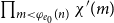 $\prod _{m \lt \varphi _{e_0}(n)} \chi '(m)$
implies
 $\chi (n) {\downarrow }$
. We can now apply
 $\mathbf{ECT}$
to find the required
 $e_1$
.
Our example follows Section 9.1 of Rogers (Reference Rogers1987).
Theorem 45.
There are oracles
 $\zeta , \kappa : \mathbb{N} \to \nabla _0 2$
such that
 $\zeta \leq _T \kappa$
and
 $\zeta \nleq _{\mathrm{wtt}} \kappa$
.
Proof.
We first define
 $\kappa$
to encode the halting problem for
 $\varphi _e(n)$
for all
 $e, n : \mathbb{N}$
, that is
 \begin{align*} \kappa (\langle e , n \rangle ) = \begin{cases} \top & \varphi _e(n) {\downarrow } \\ \bot & \text{otherwise} \end{cases} \end{align*}
We now construct
 $\zeta$
.
We first observe that for all
 $e_0, e_1, n : \mathbb{N}$
we can show the following, by repeatedly querying the oracle
 $\kappa$
.
 \begin{equation*}\bigcirc _\kappa (\mathtt {Dec}( \varphi _{e_0}(n) {\downarrow } \times \varphi _{e_1}(\langle n, \kappa (0), \ldots , \kappa (\varphi _{e_0}(n) - 1)\rangle ) \downarrow = \top )\end{equation*}
Next, by reasoning internally in the reflective subuniverse for
 $\bigcirc _\kappa$
, we can deduce the following for all
 $e_0, e_1 : \mathbb{N}$
.
 \begin{equation*} \bigcirc _\kappa \sum _{b \in 2} (b = \bot \;\leftrightarrow \ \varphi _{e_0}(\langle e_0, e_1 \rangle ) {\downarrow } \times \varphi _{e_1}(\langle \langle e_0, e_1 \rangle , \kappa (0), \ldots , \kappa (\varphi _{e_0}(\langle e_0, e_1 \rangle ) - 1)\rangle ) \downarrow = \top ) \end{equation*}
Composing with relativised projection to
 $2$
and
 $\mathtt {erase} : \bigcirc _\kappa 2 \to \nabla _0 2$
gives us
 $\zeta : \mathbb{N} \to \nabla _0 2$
, which is Turing reducible to
 $\kappa$
by construction.
Finally, suppose that we had
 $\zeta \leq _{\mathrm{wtt}} \kappa$
. By Lemma 44, there merely exists
 $e_0, e_1$
such that for all
 $n$
,
 $\zeta (n)$
and
 $\varphi _{e_1}(\langle n, \kappa (0),\ldots ,\kappa (\varphi _{e_0}(n) - 1) \rangle )$
are both defined and are equal as elements of
 $2$
. But this gives a contradiction for
 $n = \langle e_0, e_1 \rangle$
.
Remark 46. The results of this section appear in WeakTT.agdain the formalisation.
5. Markov Induction
5.1 Markov induction and Markov’s principle in HoTT
Recall that Markov’s principle is a commonly used axiom in recursive constructive mathematics that asserts the existence of numbers that can be found by unbounded search, possibly using the law of excluded middle. Formally, it is stated as follows.
Definition 47.
 $\text{Markov's principle}$
,
 $\mathbf{MP}$
, states that given a family of types
 $P : \mathbb{N} \to \mathscr{U}$
together with a proof of
 $\prod _{n : \mathbb{N}} \mathtt {Dec}(P(n))$
we have
 $\neg \neg \sum _{n : \mathbb{N}} P(n) \to \sum _{n : \mathbb{N}} P(n)$
.
For our purposes, however,
 $\mathbf{MP}$
is too weak. The reason is that it requires as antecedent a proof that every
 $P(n)$
is decidable, which in realisability semantics requires a computable function that tells us whether or not each
 $P(n)$
is true. We will give several examples of arguments where it is only possible to compute this using an oracle (i.e.,
 $f : \mathbb{N} \to \bigcirc _\chi (P(n) + \neg P(n))$
) and still wish to carry out an unbounded search. We will derive the necessary relativised version of
 $\mathbf{MP}$
from an axiom that we denote Markov induction. Although the precise formulation and applications in synthetic computability theory are new, Markov induction is equivalent to the axiom of generalised Markov’s principle for double negation, as formulated by Hofmann et al. (Reference Hofmann, van Oosten and Streicher2006). Essentially, we can extend the binary relation ‘is successor of’ from
 $\mathbb{N}$
to a binary relation on
 $\nabla _{0} \mathbb{N}$
, defined below. Markov induction says that this binary relation is well founded (Univalent Foundations Program 2013, Section 10.3). We state the axiom as an induction principle for convenience both in checking that it holds in cubical assemblies and in using it in practice.
Definition 48.
Let
 $\mu , \nu : \nabla _0 \mathbb{N}$
. We say
 $\nu$
is a
 $\text{successor}$
of
 $\mu$
if
 $\mu \downarrow = m$
implies
 $\nu \downarrow = m + 1$
for all
 $m : \mathbb{N}$
. We write
 $\mathtt {IsSuc}(\mu , \nu )$
.
Axiom 49.
 $\text{Markov induction}$
,
 $\mathbf{MI}$
states that given
 $P : \nabla _0 \mathbb{N} \to \mathscr{U}$
together with a term
 $h : \prod _{\nu : \nabla _0 \mathbb{N}} (\prod _{\mu : \nabla _0 \mathbb{N}} \mathtt {IsSuc}(\mu , \nu ) \to P(\mu )) \to P(\nu )$
, we have a section
 $s : \prod _{\nu : \nabla _0 \mathbb{N}} P(\nu )$
, together with paths witnessing the following computation rule: for all
 $\mu , \nu : \nabla _{0} \mathbb{N}$
if
 $\mathtt {IsSuc}(\mu , \nu )$
we have
 $s(\nu ) = h (\nu , \lambda \mu , x \mathpunct {.} s(\mu ))$
.
Remark 50. The computation rule was added to make the axiom more natural as an induction principle, but isn’t required for any of the results of the paper and isn’t postulated in the Agda formalisation.
Theorem 51 (Relativised Markov’s principle). Let
 $\chi : A \to \nabla _0 B$
be an oracle, a family of types
 $P : \mathbb{N} \to \mathscr{U}$
and
 $f : \prod _{n : \mathbb{N}} \bigcirc _\chi \mathtt {Dec}(P(n))$
. Then
 $\neg \neg \bigcirc _\chi (\sum _{n \in \mathbb{N}} P(n)) \;\to \; \bigcirc _\chi (\sum _{n \in \mathbb{N}} P(n))$
.
Proof.
We first show by
 $\mathbf{MI}$
that for all
 $\nu : \nabla _0 \mathbb{N}$
, we have
 $\prod _{n : \mathbb{N}} \bigcirc _\chi \mathtt {Dec}(\nu \downarrow = n) \,\to \, \bigcirc _\chi (\nu {\downarrow })$
. Suppose that the statement holds for
 $\mu$
where
 $\nu$
is a successor of
 $\mu$
and that
 $\prod _{n : \mathbb{N}} \bigcirc _\chi \mathtt {Dec}(\nu \downarrow = n)$
. Internal to the modality
 $\bigcirc _\chi$
, we split into two cases depending on whether
 $\nu \downarrow = 0$
. If
 $\nu \downarrow = 0$
, then we are done. If not, then we can show
 $\nu$
is the successor of a unique
 $\mu : \nabla _0 \mathbb{N}$
. Since
 $\mu \downarrow = n$
if and only if
 $\nu \downarrow = n + 1$
we have
 $\prod _{n : \mathbb{N}} \bigcirc _\chi \mathtt {Dec}(\mu \downarrow = n)$
, so
 $\bigcirc _\chi (\mu {\downarrow })$
by the inductive hypothesis, and so
 $\bigcirc _\chi (\nu {\downarrow })$
.
Finally, given
 $P : \mathbb{N} \to \mathscr{U}$
and
 $f : \prod _{n : \mathbb{N}} \bigcirc _\chi \mathtt {Dec}(P(n))$
, we apply the above with
 $\nu$
such that
 $\nu \downarrow = n$
when
 $n$
is least such that
 $P(n)$
. To do this, we need to show that we can decide, internally in
 $\bigcirc _{\chi }$
-modal types, whether a given
 $n$
is least such that
 $P(n)$
is true. However, this is simply an internal version of the standard fact that if
 $P(n)$
is decidable for all
 $n$
, then it is also decidable whether a given
 $n$
is least such that
 $P(n)$
.
The theorem below is the first absoluteness result we will see in this paper. Formally, we can view the interpretation of type theory in a reflective subuniverse as a syntactic translation from type theory to itself. Given a proposition, presented syntactically as a type, we can compare the translation of the proposition to the proposition itself. We say a proposition is downwards absolute if the proposition implies its translation, upwards absolute if the translation implies the original proposition and simply absolute if both directions of the implication hold.
Theorem 52.
Let
 $\bigcirc$
be a lex modality such that every
 $\bigcirc$
-connected map is
 $\neg \neg$
-dense. If
 $\mathbf{MI}$
holds in HoTT, then it also holds in the reflective subuniverse of
 $\bigcirc$
-modal types, for any oracle
 $\chi : A \to \nabla _{0} B$
. That is, Markov induction is downwards absolute for such modalities.
Proof.
Since every
 $\bigcirc$
-connected map is
 $\neg \neg$
-dense, the unit map
 $\mathbb{N} \to \bigcirc \mathbb{N}$
must be
 $\neg \neg$
-dense, and so the composition
 $\mathbb{N} \to \bigcirc \mathbb{N} \to \nabla _{0} \bigcirc \mathbb{N}$
must be
 $\nabla _{0}$
-connected. By uniqueness of factorisations for orthogonal factorisation systems, we can deduce that
 $\nabla _{0}\bigcirc \mathbb{N} \simeq \nabla _{0} \mathbb{N}$
. Note furthermore that the definition of
 $\neg \neg$
-sheaf is the same according to the internal logic of
 $\bigcirc$
-modal types as externally and that
 $\bigcirc \mathbb{N}$
is the natural number type in the reflective subuniverse for
 $\bigcirc$
. It follows that applying
 $\nabla _{0}$
to the natural number type inside
 $\bigcirc$
-modal types is the same as
 $\nabla _{0} \mathbb{N}$
externally.
Finally, note that the statement
 $\prod _{\nu : \nabla _0 \mathbb{N}} (\prod _{\mu : \nabla _0 \mathbb{N}} \mathtt {IsSuc}(\mu , \nu ) \to P(\mu )) \to P(\nu )$
is also absolute, by the same reasoning as above, and so we can apply external Markov induction to show every instance of the version internal to
 $\bigcirc$
.
Remark 53. The results of this section appear in the file OracleModality.agdaof the formalisation.
5.2 Markov induction in cubical assemblies
In this section, we will justify Markov induction by showing it holds in realisability models. As part of this, we show how to give the axiom computational meaning using the fixed point theorem.
Lemma 54.
In
 $\mathbf{Asm}$
,
 $U(\mathbb{N})$
is the
 $\neg \neg$
-sheafification of the natural number type, assuming classical logic in the metatheory.
Proof. See for example, Section 2.6.3 of van Oosten (Reference van Oosten2008).
Theorem 55. Markov induction holds in the locally cartesian closed category of assemblies, assuming classical logic in our metatheory.
Proof.
By Lemma 54, we can replace
 $\nabla _0 \mathbb{N}$
with
 $U(\mathbb{N})$
in the statement of Markov induction. Suppose that we are working in a context
 $B$
, and we have a family of types
 $P \to B \times U \mathbb{N}$
and for some
 $b \in | B |$
a map
 $f : (\prod _{\mu : U \mathbb{N}} \mathtt {IsSuc}(\mu , \nu ) \to P(b, \mu )) \to P(b, \nu )$
. Note that the function underlying the map
 $f$
gives us a choice of element
 $p_0 : P(b, 0)$
, since we vacuously have a unique element of
 $\prod _{\mu : U \mathbb{N}} \mathtt {IsSuc}(\mu , \nu ) \to P(\mu )$
. We also have functions
 $h(n) : P(b, n) \to P(b, n + 1)$
for each
 $n$
. This uniquely determines, by recursion on
 $\mathbb{N}$
in our metatheory,Footnote
7
a section
 $s$
of
 $| P | \to | B | \times \mathbb{N}$
such that
 $s(0) = p_0$
and
 $s(n + 1) = h(s(n))$
. Note that this construction is automatically stable under pullback. We only need to show how to define a realiser for
 $s$
given a realiser for
 $b$
.
Suppose that
 $d$
is a realiser for
 $f$
, as above. By the fixed point theorem (van Oosten Reference van Oosten2008, Proposition 1.3.4(ii)) we can find, uniformly in
 $d$
, a number
 $e$
such that
 $e 0 \simeq d (\lambda x, y \mathpunct {.} e 0)$
. We verify by external induction on
 $\mathbb{N}$
that
 $e$
is a realiser for
 $s$
, that is
 $e 0 \Vdash s(n)$
for all
 $n$
.
First suppose
 $n = 0$
. Note that
 $\lambda x, y \mathpunct {.} e 0$
is vacuously a realiser for
 $\prod _{\mu : U \mathbb{N}} \mathtt {IsSuc}(\mu , 0) \to P(b, \mu )$
. Hence,
 $d (\lambda x, y \mathpunct {.} e 0)$
is a realiser for
 $p_0$
and in particular
 $d (\lambda x, y \mathpunct {.} e 0){\downarrow }$
.
Next suppose
 $n = m + 1$
. By the inductive hypothesis,
 $e 0 \Vdash s(m)$
. Hence,
 $\lambda x, y \mathpunct {.} e 0 \Vdash \prod _{\mu : U \mathbb{N}} \mathtt {IsSuc}(\mu , n) \to P(b, \mu )$
. We deduce that
 $d (\lambda x, y \mathpunct {.} e 0)$
is defined and realises
 $s(n)$
. It follows that the same is true for
 $e 0$
.
Since we can find such an
 $e$
uniformly in
 $d$
, this verifies Markov induction.
Lemma 56.
In
 $\mathbf{Asm}^{\square ^{\mathrm{op}}}$
,
 $\nabla _0 \mathbb{N}$
is isomorphic to
 $\Delta U(\mathbb{N})$
.
Proof.
Observe that Definition 22 uses only the classifier for
 $\neg \neg$
-propositions, the standard type formers of dependent sums, products and identity types, and the natural number type. However, all of this is preserved by
 $\Delta$
.Footnote
8
Theorem 57. Markov induction holds in the interpretation of cubical type theory in cubical assemblies.
Proof.
By Lemma 56, we may replace
 $\nabla _0 \mathbb{N}$
with
 $\Delta U(\mathbb{N})$
in the statement of Markov induction. Given a fibration
 $P \rightarrow B \times \Delta (\nabla _0 \mathbb{N})$
together with a natural transformation
 $f : (\prod _{\mu : \nabla _0 \mathbb{N}} \mathtt {IsSuc}(\mu , \nu ) \to P(b, \mu )) \to P(b, \nu )$
, for each cube
 $[k] \in \square$
, we can restrict
 $P$
and
 $f$
to get
 $P_k \to \nabla _0 \mathbb{N}$
and
 $f_k : (\prod _{\mu : \nabla _0 \mathbb{N}} \mathtt {IsSuc}(\mu , \nu ) \to P_k(\mu )) \to P_k(\nu )$
. Applying
 $\mathbf{MI}$
in
 $\mathbf{Asm}$
gives us a family of sections
 $s_k$
for each
 $P_k$
. Furthermore, as remarked in the proof of Theorem 55, we can ensure the
 $s_k$
are uniquely determined, and so they do give us a natural transformation
 $s$
, which is a section of
 $P \to B \times \Delta (U \mathbb{N})$
.
5.3 Markov induction in synthetic computability theory
Below we give a few simple examples to illustrate the use of Markov induction via relativised Markov’s principle in synthetic computability theory. In each case, we need to construct a function computable from an oracle that at some point carries out an unbounded search. Markov induction allows us to use non-constructive reasoning to show that this gives a well-defined function that is computable from the oracle. In particular, under the appropriate conditions we can assume that particular elements of
 $\nabla _0 \mathbb{N}$
are defined. Since we are working synthetically, we simultaneously construct the function and show that it has a desired property.
Definition 58.
If
 $\chi : A \to \nabla _0 B$
, the
 $\text{graph}$
of
 $\chi$
is the function
 $\overline {\chi } : A \times B \to \nabla _0 2$
defined as below:
 \begin{align*} \overline {\chi }(a, b) := \begin{cases} 1 & \chi (a) \downarrow = b \\ 0 & \text{otherwise} \end{cases} \end{align*}
Theorem 59.
For
 $\chi : \mathbb{N} \to \nabla _0 \mathbb{N}$
, we have
 $\chi \equiv _T \overline {\chi }$
.
Proof.
It is straightforward to show
 $\overline {\chi } \leq _T \chi$
: Given
 $n, m : \mathbb{N}$
, we have
 $\bigcirc _\chi \chi (n) {\downarrow }$
. Working internally to
 $\bigcirc _\chi$
-modal types, we can decide whether
 $\chi (n) \downarrow = m$
. If it does, then
 $\overline {\chi }(n, m) \downarrow = 1$
. Otherwise,
 $\overline {\chi }(n, m) \downarrow = 0$
.
We now show that
 $\chi \leq _T \overline {\chi }$
. Suppose that we are given
 $n : \mathbb{N}$
. We will use relativised Markov’s principle, Theorem 51, to find an element of
 $\bigcirc _{\overline {\chi }} (\sum _{m : \mathbb{N}} (\chi (n) \downarrow = m))$
. It suffices to show
 $\bigcirc _{\overline {\chi }} \mathtt {Dec}(\chi (n) \downarrow = m)$
and
 $\neg \neg (\!\bigcirc _{\overline {\chi }} (\sum _{m : \mathbb{N}} \chi (n) \downarrow = m))$
. For the former, given
 $m : \mathbb{N}$
we have
 $\bigcirc _{\overline {\chi }}\overline {\chi }(n, m) {\downarrow }$
. Working internally in
 $\bigcirc _{\overline {\chi }}$
-modal types, we split into two cases depending on whether
 $\overline {\chi }(n, m) \downarrow = 1$
or
 $\overline {\chi }(n, m) \downarrow = 0$
. In the former case, we have
 $\chi (n) \downarrow = m$
and in the latter case we have
 $\neg (\chi (n) \downarrow = m)$
, as required. Finally, we have by the definition of
 $\nabla _0$
the double negation of
 $\chi (n) {\downarrow }$
, which directly gives us
 $\neg \neg (\!\bigcirc _{\overline {\chi }} (\sum _{m : \mathbb{N}} \chi (n) \downarrow = m))$
.
Although we defined oracles to be functions
 $\mathbb{N} \to \nabla _0 2$
, following a common convention in computability theory, we can see from the above theorem that in fact we can consider all oracles
 $\mathbb{N} \to \nabla _0 \mathbb{N}$
and obtain the same class of modalities, and so same definition of Turing degree.
Theorem 60.
Every surjective function
 $f : \nabla _0 \mathbb{N} \to \nabla _0 \mathbb{N}$
has a section
 $s : \nabla _0 \mathbb{N} \to \nabla _0 \mathbb{N}$
with
 $s \leq _T f$
. If
 $f$
is a bijection with inverse
 $f^{-1}$
, then
 $f^{-1} \equiv _T f$
.
Proof.
First, since
 $\nabla _0$
is a modality, every map
 $\mathbb{N} \to \nabla _0 \mathbb{N}$
extends uniquely to a map
 $\nabla _0 \mathbb{N} \to \nabla _0 \mathbb{N}$
. It follows that it suffices to construct a map
 $s : \mathbb{N} \to \nabla _0 \mathbb{N}$
such that for all
 $\mathbb{N}$
we have
 $f(s(n)) = \iota (n)$
, and that
 $s$
is Turing reducible to
 $f$
. By Lemma 35, it suffices to construct for each
 $n : \mathbb{N}$
an element of
 $\bigcirc _f (\sum _{m : \mathbb{N}} f(\iota (m)) \downarrow = n)$
. We will do this using
 $\mathbf{MP}_f$
taking
 $P(m) := f(\iota (m))$
. To do this, we need to check both
 $\prod _{m : \mathbb{N}} \bigcirc _f \mathtt {Dec}(f(\iota (m)) \downarrow = n)$
and
 $\neg \neg \sum _{m : \mathbb{N}} f(\iota (m)) = n$
. For the former, first note that we can show
 $\bigcirc _f f(\iota (m)) {\downarrow }$
. That is, internally in
 $\bigcirc _f$
-modal types, we can assume
 $f(\iota (m))$
denotes a natural number, say
 $f(\iota (m)) \downarrow = l$
. Still working internally, we can use decidable equality for
 $\mathbb{N}$
to split into two cases depending on whether
 $l = n$
. If it does, then we are done. If not, we must have
 $\neg (f(\iota (m)) \downarrow = n)$
since
 $f(\iota (m))$
cannot denote two distinct elements. Finally, to check
 $\neg \neg \sum _{m : \mathbb{N}} f(\iota (m)) = n$
, since
 $f$
is surjective, there merely exists
 $\mu : \nabla _0 \mathbb{N}$
such that
 $f(\mu ) = \iota (n)$
. It follows that
 $f(\mu ) \downarrow = n$
. By the construction of
 $\nabla _0 \mathbb{N}$
, we can show the double negation of the statement that there is
 $m$
such that
 $\mu = \iota (m)$
. From these, we derive the double negation of
 $\sum _{m : \mathbb{N}} f(\iota (m)) = n$
, as required.
We next give some useful lemmas extending relativised Markov’s principle.
Lemma 61 (‘Parallel search’). Suppose we are given two families of types
 $P, Q : \mathbb{N} \to \mathscr{U}$
, both decidable relative to an oracle
 $\chi$
such that
 $\neg \neg (\sum _{n : \mathbb{N}} P n \,+\, \sum _{n : \mathbb{N}} Q n)$
holds. Then we can deduce
 $\bigcirc _\chi (\sum _{n : \mathbb{N}} P n \,+\, \sum _{n : \mathbb{N}} Q n)$
.
Proof.
We define
 $R : \mathbb{N} \to \mathscr{U}$
by
 $R(n) := P(n) + Q(n)$
. From the decidability of
 $P$
and
 $Q$
relative to
 $\chi$
, we deduce that
 $R$
is decidable relative to
 $\chi$
. We clearly have
 $\sum _{n : \mathbb{N}} P n \,+\, \sum _{n : \mathbb{N}} Q n \to \sum _{n : \mathbb{N}} R(n)$
, and so we can deduce
 $\neg \neg \sum _{n : \mathbb{N}} R(n)$
from our assumptions. We then apply
 $\mathbf{MP}_\chi$
to deduce from this
 $\sum _{n : \mathbb{N}} R(n)$
, which implies
 $\sum _{n : \mathbb{N}} P n \,+\, \sum _{n : \mathbb{N}} Q n$
.
Lemma 62.
Let
 $\chi : A \to \nabla _0 B$
be an oracle where
 $B$
is
 $\neg \neg$
-separated. Suppose we are given
 $f, g : \mathbb{N} \to \bigcirc _\chi X$
such that
 $X$
is discrete, and
 $f \neq g$
. Then we can show
 $\bigcirc _\chi (\sum _{n : \mathbb{N}} f(n) \neq g(n))$
.
Proof.
We apply
 $\mathbf{MP}_\chi$
with
 $P(n) := f(n) \neq g(n)$
. To do this, we need to show that for all
 $w, z : \bigcirc _\chi X$
we have
 $\bigcirc _\chi \mathtt {Dec}(w = z)$
, which follows from the fact that
 $X$
is discrete and
 $\bigcirc _\chi$
is lex.
Finally, we give a technical lemma generalising Lemma 62 that will be used later in Section 8.
Lemma 63.
Suppose we are given
 $f, g, h, k : \mathbb{N} \to \bigcirc _\chi \mathbb{N}$
such that
 $\neg (f = g \times h = k)$
. Then we can show
 $\bigcirc _\chi (f \neq g + h \neq k)$
.
Proof.
We apply Lemma 61 with
 $P(n) := f(n) \neq g(n)$
and
 $Q(n) := h(n) \neq k(n)$
, and using the same argument as in Lemma 62
Remark 64. Variants of the above lemmas are proved formally in the files OracleModalities.agdaand ParallelSearch.agdaof the Agda formalisation.
6. The Axiom of Computable Choice
We give a strengthened version of Church’s thesis, which will be a synthetic version of Hyland’s axiom of generalised Church’s thesis (Hyland Reference Hyland, Troelstra and van Dalen1982, Proposition 10.4).Footnote
9
We will call the axiom computable choice to emphasise that it implies some special cases of countable choice and to draw an analogy with the axiom of continuous choice (Beeson Reference Beeson1985, Section XVI.1.3) in intuitionism. As for extended Church’s thesis we consider a synthetic version, avoiding explicit descriptions of computable partial functions by postulating functions instead. That is, we first postulate functions
 $\mathbb{N} \times \mathbb{N} \times \mathbb{N} \to \mathbb{N} + \bot$
, written
 $\varphi _{e}^k(n)$
for
 $e, k, n : \mathbb{N}$
, and further assume that
 $\varphi _e^k(n) \neq \bot$
and
 $\varphi _e^{k'}(n) \neq \bot$
implies
 $k = k'$
. Then for
 $e : \mathbb{N}$
, we write
 $\varphi _e$
for the partial function
 $\mathbb{N} \rightharpoondown \mathbb{N}$
defined by taking
 $\varphi _e(n)$
to be
 $\varphi _e^k(n)$
when there is a (necessarily unique)
 $k$
such that
 $\varphi _e^k(n) \neq \bot$
(and otherwise undefined). Finally, we use the partial functions
 $\varphi _e$
to state computable choice.
Axiom 65.
The axiom of
 $\text{computable choice}$
is as follows.
Suppose we have
 $R : \mathbb{N} \times \mathbb{N} \to \Omega _{\neg \neg }$
with
 $\neg \neg$
-stable domain. That is,
 $\sum _{n : \mathbb{N}} \exists _{m : \mathbb{N}} Rnm$
is a
 $\neg \neg$
-stable subset of
 $\mathbb{N}$
, or equivalently that we have
 \begin{equation} \prod _{n : \mathbb{N}} \left [\neg \neg \sum _{m : \mathbb{N}} R n m \;\to \; \left \| \sum _{m : \mathbb{N}} R n m \right \|\right ]. \end{equation}
Then there merely exists
 $e : \mathbb{N}$
such that for all
 $n : \mathbb{N}$
, if
 $\neg \neg \sum _{n : \mathbb{N}} R n m$
then we have
 $\varphi _{e}(n) {\downarrow }$
and
 $R n \varphi _{e}(n)$
.
Note that by allowing arbitrary relations
 $R : \mathbb{N} \times \mathbb{N} \to \Omega _{\neg \neg }$
, this is stronger than synthetic Church’s thesis in two ways:
-
(1) It allows partial functions, as long as they have
$\neg \neg$
-stable domain, generalising extended Church’s thesis, which can be recovered as the special case where
$R$
is at most single-valued. -
(2) It allows multivalued functions and so also implies a useful special case of the axiom of choice.


Having a weak form of choice available is especially useful when working with modalities generated by nullification, since the path constructors in the HIT definition can be thought of as a form of quotienting, and so choice can help us deal with maps into the nullification of a type. This will be important in Section 7.
Proposition 66. The axiom of computable choice holds in assemblies.
Proof. Similar to Proposition 10.4 of Hyland (Reference Hyland, Troelstra and van Dalen1982).
Theorem 67. There is a reflective subuniverse of the Orton–Pitts model of HoTT in cubical assemblies that satisfies computable choice and Markov induction.
Proof.
In the category of assemblies, we define two objects
 $X$
and
 $Y$
using the internal language for regular locally cartesian closed categories:
 \begin{align*} X &:= \big\{ (R, e) \in \Omega _{\neg \neg }^{\mathbb{N} \times \mathbb{N}} \times \mathbb{N} \;|\; \forall _{n : \mathbb{N}} \neg \neg \exists _{m : \mathbb{N}} R n m \,\to \, \varphi _{e}(n) {\downarrow } \,\wedge \, R n \varphi _{e(n)} \big\} \\ Y &:= \big\{ R \in \Omega _{\neg \neg }^{\mathbb{N} \times \mathbb{N}} \;|\; \forall _{n : \mathbb{N}} \neg \neg \exists _{m : \mathbb{N}} R n m \,\to \, \exists _{m : \mathbb{N}} R n m \big\} \end{align*}
Note that we have a canonical map
 $s : X \to Y$
and that computable choice precisely states that
 $s$
is surjective. In cubical assemblies, we now consider the map
 $\Delta (s) : \Delta (X) \to \Delta (Y)$
. Using the techniques of Swan and Uemura (Reference Swan and Uemura2021), we can construct a reflective subuniverse of cubical assemblies such that
 $\Delta (s)$
is homotopy surjective: note that the arguments in Section 6 of Swan and Uemura (Reference Swan and Uemura2021) go through whenever
 $A \vdash B(a)$
is a family of discrete types in the locally cartesian closed category of cubical assemblies, not necessarily definable in type theory.
Next note that
 $X$
is constructed using only type operators that are preserved by
 $\Delta$
. This ensures that
 $\Delta (X)$
agrees with the corresponding object constructed in cubical assemblies, that is,
 \begin{equation*} \Delta (X) \cong \sum _{R : \mathbb{N} \times \mathbb{N} \to \Omega _{\neg \neg }} \sum _{e : \mathbb{N}} \prod _{n : \mathbb{N}} \neg \neg \sum _{m : \mathbb{N}} R n m \,\to \, \varphi _{e}(n) {\downarrow } \,\wedge \, R n \varphi _{e(n)} \end{equation*}
On the other hand, the definition of
 $Y$
includes an existential quantifier, which makes it definitely not the same as the corresponding object
 $Y'$
defined using propositional truncation in the model of HoTT in cubical assemblies.
 \begin{equation*} Y' := \sum _{R : \mathbb{N} \times \mathbb{N} \to \Omega _{\neg \neg }} \prod _{n : \mathbb{N}} \neg \neg \sum _{m : \mathbb{N}} R n m \,\to \, \left \| \sum _{m : \mathbb{N}} R n m \right \| \end{equation*}
However, we can factor
 $\Delta (s)$
through
 $Y'$
, and the factorisation commutes with the projection to
 $\Omega _{\neg \neg }^{\mathbb{N} \times \mathbb{N}}$
.

We can show, internally in HoTT, that the projection map
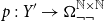 $p : Y' \to \Omega _{\neg \neg }^{\mathbb{N} \times \mathbb{N}}$
is injective. It follows that the map
 $t$
must be homotopy injective. However, in the reflective subuniverse, we now have that
 $\Delta (s) = t \circ s'$
where
 $\Delta (s)$
is a (homotopy) surjection and
 $t$
is an injection. From this, we can deduce that
 $s'$
must also be a homotopy surjection. However, this now verifies that computable choice does indeed hold in the reflective subuniverse.
Finally, since every well-supported map is also
 $\neg \neg$
-dense, we can apply Theorem 52 to see that Markov induction holds in the reflective subuniverse.
7. Relativised Computable Choice
In this section, we will show that computable choice and Markov induction together are downwards absolute. Since we have already shown that Markov induction is downwards absolute, this amounts to proving that computable choice holds in the interpretation of type theory in the reflective subuniverses for oracle modalities, assuming that Markov induction and computable choice both hold. We will refer to the statement of computable choice in the reflective subuniverse as relativised computable choice.
In order to do this, the first step is to show that we can always encode elements of
 $\bigcirc _\chi \mathbb{N}$
as natural numbers. We will use a similar construction to the one used when adding an oracle to a pca (van Oosten Reference van Oosten2008, Theorem 1.7.5) and also to the synthetic definition of Turing reducibility due to Forster et al. (Reference Forster, Kirst, Mück and Hur2023). The basic idea is that any element of
 $\bigcirc _\chi \mathbb{N}$
is either already an element of
 $\mathbb{N}$
or there is some Turing machine (coded by a natural number) that takes the value of
 $\chi (n)$
as input and then returns the code for an earlier constructed element of
 $\bigcirc _\chi \mathbb{N}$
. Since this is a coproduct of two countable sets, it is countable. We will eventually write
 $\psi$
for the resulting function
 $\mathbb{N} \to \partial \bigcirc _{\chi } \mathbb{N}$
. To get the main results of this section, we will need to have a clear picture of what it means for
 $\psi (e)$
to be defined, that is, to be a total element of
 $\bigcirc _{\chi } \mathbb{N}$
. To do this, we will use finite lists of numbers to witness that
 $\psi (e)$
is defined. We think of the length of the list as the number of oracle queries needed to complete the computation and each element of the list as the number of steps that the Turing machine takes between each query. In the below, we write finite lists of numbers as
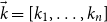 $\vec {k} = [k_1,\ldots ,k_n]$
and
 $\mathtt {List}(\mathbb{N})$
for the type of all such lists. We fix a bijection
 $\theta : \mathbb{N} \stackrel {\cong }{\to } \mathbb{N} + (\mathbb{N} \times \mathbb{N})$
.
Suppose we are given an oracle
 $\chi : \mathbb{N} \to \nabla _0 \mathbb{N}$
. We define the function
 $\psi ^\chi : \mathbb{N} \to \partial \bigcirc _\chi \mathbb{N}$
as follows. We first define elements
 $\psi ^\chi _{\vec {k}}(x)$
of
 $\bigcirc _\chi (\mathbb{N} + \{\bot \})$
for each
 $x : \mathbb{N} + (\mathbb{N} \times \mathbb{N})$
and
 $\vec {k} : \mathtt {List}(\mathbb{N})$
. We define
 $\psi ^\chi _{\vec {k}}(x)$
by induction on the length
 $m$
of the list
 $\vec {k}$
as follows. We take
 $\psi ^\chi _{[]}(x)$
to be
 $\mathtt {inl}(n)$
when
 $x = \mathtt {inl}(n)$
, and otherwise
 $\mathtt {inr}(\bot )$
. For
 $m \gt 0$
,
 $\psi ^\chi _{[k_1,\ldots ,k_m]}(\mathtt {inl}(n))$
is always
 $\mathtt {inr}(\bot )$
and we take
 $\psi ^\chi _{[k_1,\ldots ,k_m]}(\mathtt {inr}(n, e))$
to be
 $\psi ^\chi _{[k_1,\ldots ,k_{m-1}]}(\theta (\varphi _e^{k_m}(\chi (n))))$
.
We now want to define the element
 $\psi ^{\chi }(e)$
of
 $\partial \bigcirc _{\chi } \mathbb{N}$
. In order to meet the formal definition of
 $\partial \bigcirc _{\chi } \mathbb{N}$
, we need a
 $\neg \neg$
-stable proposition for the domain, together with an evaluation function
 $\psi (e) {\downarrow } \to \bigcirc _{\chi } \mathbb{N}$
. We say
 $\psi ^{\chi }(e) {\downarrow }$
when we have
 $\bigcirc _{\chi } \sum _{\vec {k} : \mathtt {List}(\mathbb{N})} \sum _{n : \mathbb{N}} \psi ^{\chi }_{\vec {k}}(\theta (e)) = \mathtt {inl}(n)$
. The evaluation function is given by applying functoriality of
 $\bigcirc _{\chi }$
to the relevant projection map. In order to check this is a valid element of
 $\partial \bigcirc _{\chi } \mathbb{N}$
, we still need to check that the domain is
 $\neg \neg$
-stable, which we do below, using relativised Markov’s principle.
Proposition 68.
 \begin{align*} \neg \neg \psi ^\chi (\theta (e)) {\downarrow } \;\to \; \bigcirc _\chi \psi ^\chi (\theta (e)) {\downarrow } \end{align*}
Proof.
Note that we have ensured that for all
 $\vec {k} : \mathtt {List}(\mathbb{N})$
, we can decide, relative to
 $\chi$
, which component of
 $\mathbb{N} + \{\bot \}$
an element of
 $\psi ^\chi _{\vec {k}}(\theta (e))$
belongs to and compute the value if it belongs to the
 $\mathbb{N}$
component, by induction on the length of the list
 $\vec {k}$
. Hence, we can apply
 $\mathbf{MP}_{\chi }$
, via a bijection
 $\mathbb{N} \cong \mathtt {List}(\mathbb{N})$
to find
 $\vec {k}$
such that
 $\psi ^\chi _{\vec {k}}(\theta (e))$
belongs to
 $\mathbb{N}$
, and thereby derive
 $\bigcirc _\chi \psi ^\chi (\theta (e)) {\downarrow }$
.
Theorem 69.
Suppose computable choice holds. Then for all
 $z : \bigcirc _\chi \mathbb{N}$
, there merely exists
 $e$
such that
 $\psi ^\chi (e) \downarrow = z$
.
Proof.
We prove this by induction on
 $z$
using Rijke et al.’s description of
 $\bigcirc _\chi \mathbb{N}$
as a HIT. Since we are proving a proposition, we only need to deal with the point constructors and can ignore the path constructors.
If
 $z$
is of the form
 $\eta (n)$
, then we can just take
 $e := \theta ^{-1}(\mathtt {inl}(n))$
.
Next suppose
 $z$
is of the form
 $\sup (n, f)$
where
 $n : \mathbb{N}$
and
 $f : \chi (n) {\downarrow } \to \bigcirc _\chi \mathbb{N}$
. By induction, we may assume that whenever
 $\chi (n) {\downarrow }$
there merely exists
 $d$
such that
 $\psi ^\chi (d) \downarrow = f(\chi (n))$
. Since
 $\psi ^\chi (d) \downarrow = f(\chi (n))$
is double negation stable by Proposition 68, we can apply computable choice here to show there exists
 $e : \mathbb{N}$
such that whenever
 $\chi (n) \downarrow = m$
, we have
 $\varphi _{e}(m) {\downarrow }$
and
 $\psi ^\chi (\varphi _{e}(m)) \downarrow = f(\chi (n))$
. It follows that
 $\psi ^\chi (\mathtt {inr}(n, e)) \downarrow = z$
, as required.
Definition 70.
Let
 $R : \mathbb{N} \times \bigcirc _{\chi } \mathbb{N} \to \Omega _{\neg \neg }$
. We say
 $e : \mathbb{N}$
 $\text{computes}$
 $R$
if for all
 $n : \mathbb{N}$
, if
 $\neg \neg \sum _{m : \mathbb{N}} R n m$
holds then
 $\psi ^\chi (\varphi _{e}(n)) \downarrow$
and
 $R n \psi ^\chi (\varphi _{e}(n))$
.
Theorem 71.
Suppose computable choice holds. Let
 $R : \mathbb{N} \times \bigcirc _{\chi }\mathbb{N} \to \Omega _{\neg \neg }$
be a
 $\neg \neg$
-stable relation such that for all
 $n : \mathbb{N}$
we have
 $\neg \neg \sum _{\mu : \bigcirc _{\chi } \mathbb{N}} R n \mu \to \| \sum _{\mu : \bigcirc _{\chi } \mathbb{N}} R n \mu \|$
. Then
 $R$
is computed by some
 $e : \mathbb{N}$
.
Proof.
We define a relation
 $R' : \mathbb{N} \times \mathbb{N} \to \Omega _{\neg \neg }$
as follows. For
 $n, m : \mathbb{N}$
, we define
 $R' n m := \psi ^\chi (m) {\downarrow } \times R n \psi ^\chi (m)$
. Note that
 $R'$
maps into
 $\neg \neg$
-stable propositions by Proposition 68.
Now
 $\sum _{m : \mathbb{N}} R' n m$
implies
 $\sum _{\mu : \bigcirc _{\chi } \mathbb{N}} R n \mu$
, since we can just take
 $\mu := \psi ^\chi (m)$
. Hence from
 $\neg \neg \sum _{m : \mathbb{N}} R' n m$
, we can deduce
 $\neg \neg \sum _{\mu : \bigcirc _{\chi } \mathbb{N}} R n \mu$
and thereby
 $\| \sum _{\mu : \bigcirc _{\chi } \mathbb{N}} R n \mu \|$
by assumption. However, we can then apply Theorem 69 to deduce that there merely exists
 $m : \mathbb{N}$
such that
 $R' n m$
.
We can therefore now apply computable choice to
 $R'$
to get the result.
Corollary 72.
Suppose that
 $\chi ' \leq _{T} \chi$
for
 $\chi , \chi ' : \mathbb{N} \to \nabla \mathbb{N}$
, then there is
 $e : \mathbb{N}$
such that for all
 $n : \mathbb{N}$
, we have
 $\chi '(n) = \mathtt {erase}(\psi ^\chi (\varphi _{e}(n)))$
.
Proof.
We apply Theorem 71 with
 $R n \mu := \chi '(n) = \mathtt {erase}(\mu )$
. We show the required hypothesis of
 $\prod _{n : \mathbb{N}} \| \sum _{\mu : \bigcirc _{\chi } \mathbb{N}} R n \mu \|$
as follows. By the assumption
 $\chi ' \leq _{T} \chi$
, we can show
 $\bigcirc _{\chi } \chi '(n) {\downarrow }$
for all
 $n : \mathbb{N}$
. Recall that
 $\chi '(n)$
is implemented as a
 $\Sigma$
-type
 $\sum _{m : \mathbb{N}} \chi '(n) \downarrow = m$
. Since
 $\bigcirc _{\chi }$
preserves
 $\Sigma$
-types and
 $R n \mu$
is already
 $\neg \neg$
-stable, and thereby
 $\bigcirc _{\chi }$
-modal, we in fact have a witness of the untruncated
 $\sum _{\mu : \bigcirc _{\chi } \mathbb{N}} R n \mu$
.
Remark 73. We can see the above corollary as a partial justification for the assertion that if
 $\chi ' \leq _{T} \chi$
in our sense, then there is an oracle Turing machine that computes
 $\chi '$
from
 $\chi$
. Strictly speaking, a complete proof would also require checking that the partial function
 $\psi ^\chi \circ \varphi _{e}$
can be implemented as an oracle Turing machine when
 $\varphi _{e}$
is the
 $e$
th computable function, and that every oracle Turing machine appears as such a function.
Corollary 74.
Assuming computable choice, for every
 $P : \bigcirc _{\chi } \mathbb{N} \to \Omega _{\neg \neg }$
the type
 $\| \sum _{\nu : \bigcirc _{\chi }\mathbb{N}} P n \|$
is
 $\bigcirc _{\chi }$
-modal.
Proof.
Suppose we are given
 $n_{0} : \mathbb{N}$
and a map
 $f : \chi (n_{0}) {\downarrow } \to \| \sum _{\bigcirc _{\chi } \mathbb{N}} P n \|$
. We define
 $R : \mathbb{N} \times \bigcirc _{\chi } \mathbb{N} \to \Omega _{\neg \neg }$
by
 $R m \nu$
when
 $\chi (n_{0}) \downarrow = m$
and
 $P \nu$
. Applying Theorem 71 tells us that there exists
 $e : \mathbb{N}$
such that if
 $\chi _{n_{0}} \downarrow = m$
, then
 $\psi ^\chi (\varphi _{e}(m)) \downarrow$
and
 $P \psi ^\chi (\varphi _{e}(m))$
. Given such an
 $e$
, we define
 $f' : \chi (n_{0}) {\downarrow } \to \bigcirc _{\chi } \mathbb{N}$
by taking
 $f'(m)$
to be
 $\psi ^\chi (\varphi _{e}(m))$
. We can now apply the fact that
 $\bigcirc _{\chi } \mathbb{N}$
is modal to find the diagonal filler, which is an element
 $\nu$
of
 $\bigcirc _{\chi } \mathbb{N}$
such that if
 $\chi (n_{0}) {\downarrow }$
, then
 $\nu = \psi ^\chi (\varphi _{e}(m))$
. Since
 $P$
is
 $\neg \neg$
-stable and
 $\chi (n_{0}) {\downarrow }$
is
 $\neg \neg$
-dense, this implies that we in fact have
 $P \nu$
. Hence, we have an element of
 $\| \sum _{\nu : \bigcirc _{\chi } \mathbb{N}} P \nu \|$
, as required.
Remark 75. In general we expect that if we are given an accessible modality generated by projective types, then
 $-1$
-truncation preserves modal types. In this case, we are not able to show in cubical assemblies that the proposition
 $\chi (n) {\downarrow }$
is projective, but using computable choice we have used a related argument to show the special case that
 $\| \bigcirc _{\chi } \mathbb{N} \|$
is
 $\bigcirc _{\chi }$
-modal.
Corollary 76. Suppose that both Markov induction and computable choice both hold. Then they also both hold in the reflective subuniverse corresponding to any oracle modality. That is, together they are downwards absolute for oracle modalities.
Proof.
We have already seen that Markov induction holds in Theorem 52. The remainder of the theorem is a proof that computable choice holds internally. By unfolding the interpretation of the statement in the subuniverse, we can see that this almost follows directly from Theorem 71. The only issue is that the interpretation of the hypothesis (1) is
 $\prod _{n : \mathbb{N}} \neg \neg \sum _{m : \mathbb{N}} R n m \to \bigcirc _{\chi } \| \sum _{m : \mathbb{N}} R n m \|$
, whereas we need a statement of the form
 $\prod _{n : \mathbb{N}} \neg \neg \sum _{m : \mathbb{N}} R' n m \to \| \sum _{\mu : \bigcirc _{\chi } \mathbb{N}} R' n \mu \|$
to apply Theorem 71. However, Corollary 74 tells us that
 $\| \sum _{\mu : \bigcirc _{\chi } \mathbb{N}} \prod _{m : \mathbb{N}}\mu \downarrow = m \to R n m \|$
is
 $\bigcirc _{\chi }$
-modal, and so we can eliminate out to get a map
 $\bigcirc _{\chi } \| \sum _{m : \mathbb{N}} R n m \| \to \| \sum _{\mu : \bigcirc _{\chi } \mathbb{N}} \prod _{m : \mathbb{N}}\mu \downarrow = m \to R n m \|$
. We can then apply Theorem 71 with
 $R'n \mu := \mu \downarrow = m \to R n m$
to get the result.
The above corollary demonstrates that synthetic proofs using Markov induction and computable choice can be ‘relativised to an oracle’. That is, they can be carried out internally in the reflective subuniverse corresponding to an oracle. This corresponds to the concept of relativisation in computability theory, which is the idea that many proofs about computable functions apply equally well to functions computable relative to an oracle.
Although we needed the full strength of computable choice to show that any form of Church’s thesis holds in the reflective subuniverse, once we have it we can derive the other, weaker versions, such as relativised versions of extended Church’s thesis and Church’s thesis itself:
Corollary 77 (Relativised extended Church’s thesis). For any function
 $f : \mathbb{N} \to \partial \bigcirc _{\chi } \mathbb{N}$
, there exists
 $e : \mathbb{N}$
such that for all
 $n$
, if
 $f(n) {\downarrow }$
, then
 $\psi ^\chi (\varphi _{e}(n)) \downarrow = f(n)$
.
Proof.
We apply relativised computable choice with
 $R n \mu := f(n) \downarrow = \mu$
.
7.1 Turing jump
An important corollary of relativised computable choice is that we can now relativise the construction of the halting set and proof that it is non-computable (Proposition 40). This gives us the following definition of Turing jump.
Definition 78.
Given
 $\chi : \mathbb{N} \to \nabla _0 2$
, we define the
 $\text{Turing jump}$
 $\hat {\chi } : \mathbb{N} \to \nabla _0 2$
as follows.
 \begin{align*} \hat {\chi }(n) := \begin{cases} 1 & \psi ^\chi (\varphi _n(n)) \downarrow = \eta (0) \\ 0 & \textit{otherwise} \end{cases} \end{align*}
Theorem 79.
Suppose computable choice and Markov induction. Then
 $\hat {\chi } \nleq _T \chi$
.
Proof.
Suppose that we did have
 $\hat {\chi } \leq _T \chi$
. This is precisely a witness of
 $\prod _{n : \mathbb{N}} \bigcirc _\chi (\hat {\chi }(n){\downarrow })$
, and recall that
 $\hat {\chi }(n){\downarrow } := \sum _{m : 2} (\hat {\chi }(n) \downarrow = m)$
. By Lemma 1.24 of Rijke et al. (Reference Rijke, Shulman and Spitters2020), we have
 $\bigcirc _\chi (\hat {\chi }(n){\downarrow }) \simeq \sum _{z : \bigcirc _\chi 2} \bigcirc _\chi \hat {\chi }(n) \downarrow = m$
. We can extract from this a map
 $f : \mathbb{N} \to \bigcirc _\chi 2$
together with a proof that
 $\mathtt {erase}(f(n)) = \hat {\chi }(n)$
for all
 $n$
, that is
 $\hat {\chi }$
factors through
 $\mathtt {erase} : \bigcirc _\chi 2 \to \nabla _0 2$
. We then have that
 $f$
must be computable by some
 $e : \mathbb{N}$
. However, this gives a contradiction, since we have
 $\psi (\varphi _e(e)) \downarrow = f(e) \neq \psi (\varphi _e(e))$
.
7.2 Local continuity
We can also use relativised computable choice to give us a ‘local continuity’ theorem for our definition of Turing reducibility, verifying that each oracle computation only requires a finite number of queries:
Theorem 80.
Let
 $\chi$
be an oracle
 $\mathbb{N} \to \nabla _0 \mathbb{N}$
. Suppose
 $\psi ^\chi _{[k_1,\ldots ,k_n]}(e) {\downarrow }$
. Then we can deduce the following.
 \begin{align*} \bigcirc _\chi \bigg(\sum _{l \in \mathtt {List} \mathbb{N}} \prod _{\chi ' : \mathbb{N} \to \nabla _0 \mathbb{N}} &\bigg(\prod _{m \in l} \chi '(m) = \chi (n)\bigg) \quad \to \quad \\ & \psi ^{\chi '}_{[k_1,\ldots ,k_n]}(e) {\downarrow } \times \mathtt {erase}(\psi ^{\chi '}(e)) = \mathtt {erase}(\psi ^\chi (e))\bigg) \end{align*}
Proof.
We prove this by induction on the length
 $m$
of the list
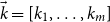 $\vec {k} = [k_1,\ldots ,k_m]$
.
For
 $\vec {k} = []$
, we do not require the oracle and can just take
 $l = []$
. We then have
 $e = \mathtt {inl}(n)$
and
 $\mathtt {erase}(\psi _{\chi '}(e)) = \iota (n) = \mathtt {erase}(\psi _{\chi }(e))$
.
For
 $\vec {k} = [k_1,\ldots ,k_{m-1},k_{m}]$
, we have
 $e = \mathtt {inr}(n, e')$
and
 $\chi (n) {\downarrow }$
implies
 $\varphi _e(\chi (n)) {\downarrow }$
with
 $\psi ^\chi _{\vec {k}}(e) = \psi ^\chi _{[k_1,\ldots ,k_{m-1}]}(\theta (\varphi _{e'}^{k_m}(\chi (n))))$
. Since we are now working relative to
 $\chi$
, we can in fact assume
 $\chi (n) {\downarrow }$
. By the inductive hypothesis, applied with
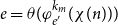 $e = \theta (\varphi _{e'}^{k_m}(\chi (n)))$
, we have, relative to
 $\chi$
,
 $l : \mathtt {List}(\mathbb{N})$
such that
 $\prod _{x \in l} \chi '(x) = \chi (x)$
implies
 $\mathtt {erase}(\psi ^{\chi '}(\theta (\varphi _{e'}^{k_m}(\chi (n))))) = \mathtt {erase}(\psi ^\chi (\theta (\varphi _{e'}^{k_m}(\chi (n)))))$
. We append
 $n$
to
 $l$
to obtain a new list
 $l'$
. If
 $\prod _{k \in l'}\chi '(k) = \chi (k)$
, then we can calculate as follows:
 \begin{align*} \mathtt {erase}\Big(\psi ^{\chi '}_{\vec {k}}(e)\Big) &= \mathtt {erase}\Big(\psi ^{\chi '}_{[k_1,\ldots ,k_{m-1}]}\Big(\theta \Big(\varphi ^{k_m}_{e'}(\chi '(n))\Big)\Big)\Big) \\ &= \mathtt {erase}\Big(\psi ^{\chi '}_{[k_1,\ldots ,k_{m-1}]}\Big(\theta \Big(\varphi ^{k_m}_{e'}(\chi (n))\Big)\Big)\Big) \\ &= \mathtt {erase}\Big(\psi ^{\chi }_{[k_1,\ldots ,k_{m-1}]}\Big(\theta \Big(\varphi ^{k_m}_{e'}(\chi (n))\Big)\Big)\Big) \\ &= \mathtt {erase}\big(\psi ^{\chi }_{\vec {k}}(e)\big) \end{align*}
Corollary 81.
For any
 $\chi : \mathbb{N} \to \nabla _0 \mathbb{N}$
and any
 $z : \bigcirc _\chi \mathbb{N}$
, there merely exists
 $e : \mathbb{N}$
such that we can compute, relative to
 $\chi$
, a finite list
 $l : \mathtt {List} (\mathbb{N})$
such that whenever
 $\chi '(m) = \chi (m)$
for all
 $m \in l$
we have
 $\psi ^{\chi '}(e) {\downarrow }$
with
 $\mathtt {erase}(\psi ^{\chi '}(e)) = \mathtt {erase}(z)$
.
Proof.
By Theorem 69, there merely exists
 $e$
such that
 $\psi ^\chi (e) \downarrow = z$
. By Proposition 68, we can compute, relative to
 $\chi$
, the finite list
 $\vec {k}$
such that
 $\psi ^\chi _{\vec {k}}(\theta (e)) = z$
. However, we can now apply Theorem 80.
Remark 82. The results of this section appear in RelativisedCC.agdain the formalisation.
8. Computability and (Higher) Group Theory
In this section, we give an example of the new kind of proof technique that becomes possible by combining the definition of oracle modality in this paper with existing results in HoTT. Our example is a synthetic proof that two Turing degrees are equal as soon as they induce isomorphic permutation groups on
 $\mathbb{N}$
. From computability theory, our proof will make use of Lemma 63. From HoTT, we will use an approach to group theory due to Buchholtz et al. (Reference Buchholtz, van Doorn and Rijke2018) (see also Bezem et al. Reference Bezem, Buchholtz, Cagne, Dundas and Grayson2026).
As Buchholtz et al. showed, there is an equivalence and so equality between the category of groups and the category of pointed, connected,
 $1$
-truncated types. Based on this idea, they suggested an approach to group theory where standard constructions in group theory are replaced with arguments that work directly with pointed, connected,
 $1$
-truncated types. As they point out, this approach has the advantage of being easier to generalise to higher dimensions. In particular to define
 $\infty$
-groups, we simply drop the requirement of
 $1$
-truncation. This approach to group theory can help with formalisation, since the group multiplication operation is not extra data that we need to keep track of, but concatenation of paths, which is already implicit in any type. Furthermore, certain constructions in group theory are more natural from this point of view. Of particular relevance to this proof, the permutation group of a type is just the connected component of that type in the universe, and wreath product can be simply described as a
 $\Sigma$
-type (Buchholtz et al. Reference Buchholtz, van Doorn and Rijke2018, Sections 4.1 and 4.6). We will give a direct proof based on these ideas that Turing degrees are equivalent when they induce isomorphic permutation groups, spelling out the details and with a few further simplifications. We point out that this technique makes essential use of types that are not
 $0$
-truncated and so illustrates the benefits of using cubical assemblies as our semantics rather than the effective topos.
We recall below construction of homotopy group of a pointed space, which is used for one direction of the equivalence between the two definitions of group.
Definition 83.
Let
 $X$
be a type and
 $x : X$
. The
 $\text{loop space}$
at
 $x$
, written
 $\Omega (X, x)$
, is the identity type
 $x =_X x$
. The
 $\text{homotopy group}$
at
 $x$
,
 $\pi _1(X, x)$
, is the
 $0$
-truncation
 $\| \Omega (X, x) \|_0$
with group multiplication defined as the composition of paths.
Proposition 84.
Every pointed map
 $f : (X, x) \to (Y, y)$
induces a group homomorphism
 $\pi _0(f) : \pi _1(X, x) \to \pi _1(Y, y)$
. Every map
 $f : X \to Y$
induces a group homomorphism
 $\pi _1(X, x) \to \pi _1(Y, f(x))$
.
Theorem 85.
Suppose we are given oracles
 $\chi , \chi ' : \mathbb{N} \to \nabla _0 2$
together with a group isomorphism
 $\alpha : \nabla _0(\Omega (\mathscr{U}, \bigcirc _\chi \mathbb{N})) \cong \nabla _0(\Omega (\mathscr{U}, \bigcirc _{\chi '} \mathbb{N}))$
. Then we have
 $\neg \neg (\chi ' \equiv _T \chi )$
.
To prove this, we will make use of the functions
 $F_A$
, for
 $A : \mathscr{U}$
, and
 $D$
defined below.

The first key point is that
 $D \circ F_A$
induces an embedding of groups, which we show in two steps.
Lemma 86.
For any types
 $A, X : \mathscr{U}$
, we have an equivalence
 $\mathtt {fibre}_{D \circ F_A}(X) \simeq A^X$
Proof.
Write
 $\mathscr{U}/A$
for the ‘slice category over
 $A$
’, that is, the type
 $\sum _{W : \mathscr{U}} A^W$
. Note that we have an equivalence
 $e : \mathscr{U}^A \stackrel {\simeq }{\to } \mathscr{U}/A$
where
 $D \circ F_A = \operatorname {dom} \circ e$
. Hence, it suffices to show that
 $\mathtt {fibre}_{\operatorname {dom}}(X) \simeq A^X$
, which we do as follows:
 \begin{align*} \mathtt {fibre}_{\operatorname {dom}}(X) &\simeq \sum _{\sum _{W : \mathscr{U}} A^W} W = X \\ &\simeq \sum _{\sum _{W : \mathscr{U}} W = X} A^W \\ &\simeq A^X \end{align*}
Lemma 87.
Suppose that
 $A$
and
 $X$
are sets. The map
 $D \circ F_A : \Omega (\mathscr{U}^{A}, \lambda a \mathpunct {.} X) \to \Omega (\mathscr{U}, A \times X)$
defined by action on paths is an embedding.
Proof.
It suffices to show that
 $K := \mathtt {fibre}_{D \circ F_A} (A \times X)$
is
 $0$
-truncated. However, by Lemma 86,
 $K$
is equivalent to the exponential
 $A^{A \times X}$
, which is
 $0$
-truncated by the assumption that
 $A$
and
 $X$
are
 $0$
-truncated.
The second key point is that we can view the wreath products of symmetry groups as loop spaces in
 $\sum _{X : \mathscr{U}} \mathscr{U}^{X}$
. In particular, we can show by general arguments that concatenation of paths behaves as we would expect for the usual group theoretic definition of wreath product.
More formally, we note that by based path induction for each path
 $p : A = B$
and each
 $X : A \to \mathscr{U}$
we can define a path
 $\tilde {p} : F_A(X) = F_B(X \circ p^\ast )$
. We then have the following lemma.
Lemma 88.
Suppose we are given
 $A, X : \mathscr{U}$
together with paths
 $p : A = A$
and
 $q : A \to (X = X)$
. Note that
 $q \circ p^\ast$
also has type
 $A \to X = X$
. We then have
 $F_A(q \circ p^\ast ) = \tilde {p}^{-1} \cdot F_A(q) \cdot \tilde {p}$
.
Proof.
This is a special case of the following more general statement that we can prove by based path induction on
 $p$
. Suppose
 $A, B : \mathscr{U}$
,
 $X : \mathscr{U}$
,
 $p : A = B$
and
 $q : A \to X = X$
. Then we have the following commutative square in
 $\sum _{Z : \mathscr{U}} \mathscr{U}^Z$
:

Write
 $\mathbb{Z}_\bot$
for
 $\mathbb{Z} + 1$
. We are going to apply the above construction with
 $A := \mathbb{Z}_{\bot }$
. We consider the point
 $\lambda x \mathpunct {.} \bigcirc _{\chi } 2$
of
 $\mathscr{U}^{\mathbb{Z}_{\bot }}$
. In particular, note that the action on paths of
 $F_{A}$
and
 $D$
gives us group homomorphisms as follows:
 \begin{align*} \Omega \big(\mathscr{U}^{\mathbb{Z}_{\bot }}, \lambda x \mathpunct {.} \bigcirc _{\chi } 2\big) \stackrel {F_{\mathbb{Z}_\bot }}{\longrightarrow } \Omega \left (\sum _{{A : \mathscr{U}}}\mathscr{U}^{A}, (\mathbb{Z}_{\bot }, \lambda x \mathpunct {.} \bigcirc _{\chi } 2)\right ) \stackrel {D}{\longrightarrow } \Omega \left (\mathscr{U}, \mathbb{Z}_{\bot } \times \bigcirc _{\chi } 2\right ) \end{align*}
We will use the following permutations of
 $\mathbb{Z}_\bot$
in our proofs. For convenience, we will write the corresponding loops of
 $\mathbb{Z}_\bot$
in
 $\mathscr{U}$
as
 $s_\bot$
and
 $\tau _n$
for
 $n : \mathbb{Z}$
, so the equivalences will be the transport operations
 $s_\bot ^\ast$
and
 $\tau _n^\ast$
. We take
 $s_\bot ^\ast : \mathbb{Z}_\bot \simeq \mathbb{Z}_\bot$
to be the permutation of
 $\mathbb{Z}_\bot$
that shifts by
 $1$
on the
 $\mathbb{Z}$
component and is the identity on the
 $1$
component. For
 $n : \mathbb{Z}$
, we take
 $\tau _n^\ast$
to be the permutation
 $\mathbb{Z}_\bot \simeq \mathbb{Z}_\bot$
that swaps
 $n : \mathbb{Z}$
with the unique element of
 $1$
, and otherwise is the identity.
Lemma 89.
For all
 $n$
, we have
 $\tau _n = s_\bot ^{-n} \cdot \tau _0 \cdot s_\bot ^{n}$
.
Proof. It is straightforward to show the corresponding statement for equivalences directly.
Next, note that we can encode
 $\chi$
as two elements
 $k, k'$
of
 $\Omega (\mathscr{U}^{\mathbb{Z}_\bot }, \lambda x \mathpunct {.} \bigcirc _\chi 2)$
. First, given
 $n : \mathbb{N}$
we define
 $q : \mathbb{N} \to \Omega (\mathscr{U}, \bigcirc _\chi 2)$
internally in
 $\bigcirc _\chi$
-modal types as follows, writing
 $\mathtt {not}$
for the non-trivial path
 $2 = 2$
swapping the two elements:
 \begin{align*} q(n) = \begin{cases} 1_2 & \chi (n) = 0 \\ \mathtt {not} & \chi (n) = 1 \end{cases} \end{align*}
We then define
 $k, k' : \mathbb{Z}_\bot \to \Omega (\mathscr{U}, \bigcirc _\chi 2)$
as follows:
 \begin{align*} k(x) = \begin{cases} q(| x |) & x \in \mathbb{Z} \\ \mathtt {not} & x \in 1 \end{cases} \qquad k'(x) = \begin{cases} q(|x|) & x \in \mathbb{Z} \\ 1_{2} & x \in 1 \end{cases} \end{align*}
Note that we have defined
 $k, k', \tau _n$
to ensure that the following lemma holds.
Lemma 90.
For all
 $n$
, we have
 $\chi (n) \downarrow = 0$
iff
 $k \neq k \circ \tau _n$
, and
 $\chi (n) \downarrow = 1$
iff
 $k' \neq k' \circ \tau _n$
.
We now combine the above lemmas together to get our key lemma. The idea is that we can construct the Turing reduction once we have
 $\alpha (z_i){\downarrow }$
for all elements of a finite list
 $z_1,\ldots ,z_n$
, where we recall that
 $\alpha$
is our assumed isomorphism
 $\nabla _0(\Omega (\mathscr{U}, \bigcirc _\chi \mathbb{N})) \cong \nabla _0(\Omega (\mathscr{U}, \bigcirc _{\chi '}\mathbb{N}))$
. Instead of using
 $\alpha$
directly, we state the key lemma for an embedding from
 $\Omega (\mathscr{U}, \mathbb{Z}_\bot \times \bigcirc _{\chi } 2)$
to
 $\nabla _0 (\Omega (\mathscr{U}, \bigcirc _{\chi '} \mathbb{N}))$
.
Lemma 91.
Suppose we have an embedding of groups
 $\beta$
from
 $\Omega (\mathscr{U}, \mathbb{Z}_\bot \times \bigcirc _{\chi } 2)$
to
 $\nabla _0(\Omega (\mathscr{U}, \bigcirc _{\chi '} \mathbb{N}))$
. Suppose that
 $\beta (D(F_{\mathbb{Z}_\bot }(k))) {\downarrow }$
,
 $\beta (D(F_{\mathbb{Z}_\bot }(k'))) {\downarrow }$
,
 $\beta (D(\tilde {\tau }_0)) {\downarrow }$
and
 $\beta (D(\widetilde {s_\bot })) {\downarrow }$
. Then,
 $\chi \leq _T \chi '$
.
Proof.
By Lemma 89, we can show that
 $\beta (D(\tilde {\tau }_n)) {\downarrow }$
for all
 $n$
. But by Lemma 88, we know
 $F_{\mathbb{Z}_\bot }(k \circ \tau _n^\ast ) = \tilde {\tau }_n^{-1} \cdot F_{\mathbb{Z}_\bot }(k) \cdot \tilde {\tau }_n$
, and so also
 $\beta (D(F_{\mathbb{Z}_\bot }(k \circ \tau _n^\ast ))) {\downarrow }$
and similarly
 $\beta (D(F_{\mathbb{Z}_\bot }(k' \circ \tau _n^\ast ))) {\downarrow }$
. Since
 $\bigcirc _\chi$
is lex, it preserves hlevel (Rijke et al. Reference Rijke, Shulman and Spitters2020, Corollary 3.9), and so we can apply Lemma 87 to see that
 $D \circ F_{\mathbb{Z}_\bot }$
is an embedding of groups.
Therefore by Lemma 90, we can see that
 $\chi (n) \downarrow = 0$
iff
 $\beta (D(F_{\mathbb{Z}_\bot }(k))) \neq \beta (D(F_{\mathbb{Z}_\bot }(k \circ \tau _n^\ast )))$
and
 $\chi (n) \downarrow = 1$
iff
 $\beta (D(F_{\mathbb{Z}_\bot }(k'))) \neq \beta (D(F_{\mathbb{Z}_\bot }(k' \circ \tau _n^\ast )))$
. However, we can view the elements of
 $\Omega (\mathscr{U}, \bigcirc _{\chi '} \mathbb{N})$
as functions computable in
 $\chi '$
, and so apply Lemma 63 to deduce
 $\bigcirc _{\chi '} (\beta (D(F_{\mathbb{Z}_\bot }(k))) \neq \beta (D(F_{\mathbb{Z}_\bot }(k \circ \tau _n^\ast ))) + \beta (D(F_{\mathbb{Z}_\bot }(k'))) \neq \beta (D(F_{\mathbb{Z}_\bot }(k' \circ \tau _n^\ast ))))$
and thereby
 $\bigcirc _{\chi '} \chi (n) {\downarrow }$
.
Lemma 92.
There is an embedding of groups
 $\Omega (\mathscr{U}, \mathbb{Z}_\bot \times \bigcirc _{\chi } 2) \hookrightarrow \nabla _0(\Omega (\mathscr{U}, \bigcirc _{\chi '} \mathbb{N}))$
.
Proof.
First note that in general, for types
 $A$
and
 $B$
and a modality
 $\bigcirc$
the functoriality of
 $\bigcirc$
gives us a canonical map from
 $A \simeq B$
to
 $\bigcirc A \simeq \bigcirc B$
. When
 $B$
is
 $\bigcirc$
-separated and
 $\bigcirc$
is lex, this map is injective. Hence, we have a subgroup inclusion from
 $\Omega (\mathscr{U}, \mathbb{Z}_\bot \times \bigcirc _\chi 2)$
to
 $\Omega (\mathscr{U}, \bigcirc _\chi (\mathbb{Z}_\bot \times \bigcirc _\chi 2))$
. However, we have an evident sequence of equivalences as follows:
 \begin{equation*} \bigcirc _\chi (\mathbb{Z}_\bot \times \bigcirc _\chi 2) \quad \simeq \quad \bigcirc _\chi \mathbb{Z}_\bot \times \bigcirc _\chi 2 \quad \simeq \quad \bigcirc _\chi (\mathbb{Z}_\bot \times 2) \quad \simeq \quad \bigcirc _\chi \mathbb{N} \end{equation*}
Hence, we have
 $\Omega (\mathscr{U}, \bigcirc _\chi (\mathbb{Z}_\bot \times \bigcirc _\chi 2)) \simeq \Omega (\mathscr{U}, \bigcirc _\chi \mathbb{N})$
.
Since
 $\Omega (\mathscr{U}, \bigcirc _\chi \mathbb{N})$
is
 $\neg \neg$
-separated, the unit map from
 $\Omega (\mathscr{U}, \bigcirc _\chi \mathbb{N})$
to
 $\nabla _0 \Omega (\mathscr{U}, \bigcirc _\chi \mathbb{N})$
is injective.
Composing all these together gives the embedding of groups from
 $\Omega (\mathscr{U}, \mathbb{Z}_\bot \times \bigcirc _{\chi } 2)$
to
 $\nabla _0(\Omega (\mathscr{U}, \bigcirc _{\chi } \mathbb{N}))$
.
Proof of Theorem
85. Clearly, it suffices to show
 $\neg \neg \chi \leq _T \chi '$
, since we can then also show
 $\neg \neg \chi ' \leq _T \chi$
by symmetry and thereby deduce
 $\neg \neg \chi ' \equiv _T \chi$
.
By composing the embedding from Lemma 92 with the assumed isomorphism
 $\alpha$
between
 $\nabla _0(\Omega (\mathscr{U}, \bigcirc _\chi \mathbb{N}))$
and
 $\nabla _0(\Omega (\mathscr{U}, \bigcirc _{\chi '} \mathbb{N}))$
, we get an embedding
 $\beta$
from
 $\Omega (\mathscr{U}, \mathbb{Z}_\bot \times \bigcirc _{\chi } 2)$
to
 $\nabla _0(\Omega (\mathscr{U}, \bigcirc _{\chi '} \mathbb{N}))$
.
From Lemma 91, we can deduce
 $\neg \neg \chi ' \equiv _T \chi$
from the double negation of the product of the finite list of assumptions
 $\beta (D(F_{\mathbb{Z}_\bot }(k))) {\downarrow }$
,
 $\beta (D(F_{\mathbb{Z}_\bot }(k'))) {\downarrow }$
,
 $\beta (D(\tilde {\tau }_0)) {\downarrow }$
and
 $\beta (D(\tilde {s_\bot })) {\downarrow }$
. However, since the list is finite, the double negation of its product is the same as the product of the double negations of each of its elements. However, we can prove the double negation of each element of the list, and so we are done.
Remark 93. A proof of a variant of the key Lemma 91 appears in PermutationGroups.agdain the formalisation.
9. Some Non-Topological Modalities
In this section, we will give some examples of modalities based on oracle modalities, but combined with higher types. For this, we will use a general construction due to Christensen et al. (Reference Christensen, Opie, Rijke and Scoccola2020).
Definition 94 (Christensen–Opie–Rijke–Scoccola). Let
 $\bigcirc$
be a modality. The
 $\text{suspension}$
of
 $\bigcirc$
is the (necessarily unique) modality
 $\Sigma \bigcirc$
such that a type
 $A$
is
 $\Sigma \bigcirc$
-modal if and only if it is
 $\bigcirc$
-separated.
We write
 $\bigcirc ^{(n)}$
for the result of iterating the suspension
 $n$
times. That is,
 $\bigcirc ^{(0)} = \bigcirc$
and
 $\bigcirc ^{(n + 1)} = \Sigma (\!\bigcirc ^{(n)})$
.
Although Christensen et al. showed that suspension modalities exist in general, we will only need the following easier special case.
Proposition 95.
Suppose that
 $\bigcirc$
is the nullification of a family of types
 $B : A \to \mathscr{U}$
. Then
 $\Sigma \bigcirc$
is the nullification of the family
 $\Sigma B : A \to \mathscr{U}$
, defined by mapping
 $a : A$
to
 $\Sigma (B(a))$
, the suspension of
 $B(a)$
.
Although this is an entirely general definition, we can view it as a natural construction in computability theory as follows. We can think of
 $\bigcirc _{\chi } X$
as the result of adding new points to
 $X$
. Namely, we think of
 $X$
as only containing computable elements, and
 $\bigcirc _{\chi } X$
as also containing new points that can be computed using the oracle
 $\chi$
. On the other hand, in
 $\bigcirc ^{(1)}_{\chi } X$
, we can use the oracle only to compute new paths, while the points are left unaffected. More generally, in
 $\bigcirc ^{(n)}_{\chi }$
we can use the oracle
 $\chi$
to compute new
 $m$
-cells for
 $m \geq n$
, leaving lower dimensions the same.
We can make this precise through the following arguments. We first consider the easier case of showing that lower dimensions are unaffected. We first observe that the case where
 $n \gt m + 1$
holds in general for purely formal reasons, using the following lemma.
Lemma 96.
For any modality
 $\bigcirc$
and any type
 $X$
, the unit map
 $\eta ^{(n)} : X \to \bigcirc ^{(n)} X$
is
 $(n - 2)$
-connected.
Proof.
We have
 $\bigcirc \leq _{T} \| - \|_{-2}$
. Hence,
 $\bigcirc ^{(n)} \leq _{T} \| - \|_{-2}^{(n)} = \| - \|_{(n - 2)}$
. Hence,
 $\eta ^{(n)}$
is
 $\| - \|_{(n - 2)}$
-connected.
Proposition 97.
If
 $n - k \geq 2$
, then
 $\pi _{k}(\!\bigcirc ^{(n)} X) = \pi _{k}(X)$
for all
 $X$
.
Proof.
By Lemma 96, the unit map
 $Y \to \bigcirc ^{(n - k)} Y$
is
 $0$
-connected for any
 $Y$
. The truncation map
 $\bigcirc ^{(n - k)} Y \to \| \bigcirc ^{(n)} Y \|_{0}$
is also
 $0$
-connected. Hence, the composition
 $Y \to \| \bigcirc ^{(n - k)} Y \|_{0}$
is
 $0$
-connected. Hence,
 $\| \bigcirc ^{(n - k)} Y \|_{0} = \| Y \|_{0}$
by uniqueness of factorisations. Applying this with
 $Y = \Omega ^{k} X$
, we can reason as follows:
 \begin{align*} \pi _{k}\big(\!\bigcirc ^{(n)} X\big) &= \| \Omega ^{k} \big(\!\bigcirc ^{(n)} X\big) \|_{0} \\ &= \| \bigcirc ^{(n - k)} \Omega ^{k} X \|_{0} \\ &= \| \Omega ^{k} X \|_{0} \\ &= \pi _{k}(X) \end{align*}
The case
 $n = k + 1$
is harder and requires the additional assumption that we already know
 $\pi _{k}(A)$
is
 $\neg \neg$
-separated:
Lemma 98.
Suppose that
 $\| X \|_{0}$
is
 $\nabla$
-separated. Then for any modality
 $\bigcirc$
with
 $\bigcirc \leq _{T} \nabla$
, we have
 $\| \bigcirc ^{(1)} X \|_{0} = \| X \|_{0}$
.
Proof.
We have in any case a canonical map
 $\| X \|_{0} \to \| \bigcirc ^{(1)} X \|_{0}$
. The map is surjective, that is,
 $-1$
-connected, by the same argument as in Proposition 97. Hence, we just need to check that the map is injective. Since truncation is surjective, it suffices to show that for
 $x, y : X$
, if
 $| \eta ^{\bigcirc ^{(1)}}(x) |_{0} = | \eta ^{\bigcirc ^{(1)}}(y) |_{0}$
, then
 $| x |_{0} = | y |_{0}$
. However, we can calculate
 \begin{align*} | \eta ^{\bigcirc ^{(1)}}(x) |_{0} = | \eta ^{\bigcirc ^{(1)}}(y) |_{0} &= \| \eta ^{\bigcirc ^{(1)}}(x) = \eta ^{\bigcirc ^{(1)}}(y) \|_{-1} \\ &= \| \bigcirc (x = y) \|_{-1} \\ &\leq \| \nabla (x = y) \|_{-1} \\ &\leq \| \nabla (|x|_{0} = |y|_{0}) \|_{-1} \\ &= \| |x|_{0} = |y|_{0} \|_{-1} \\ &= |x|_{0} = |y|_{0} \end{align*}
Proposition 99.
Suppose that
 $X$
is a type such that
 $\pi _{n}(X)$
is
 $\neg \neg$
-separated for some
 $n \geq 1$
. Then
 $\pi _{n}(\!\bigcirc ^{(n + 1)} X) = \pi _{n}(X)$
.
Proof. We first observe the following equality.
 \begin{align*} \pi _{n}\big(\!\bigcirc ^{(n + 1)} X\big) &= \| \Omega ^{n}\big(\!\bigcirc ^{(n + 1)} X\big) \|_{0} \\ &= \| \bigcirc ^{(1)} \Omega ^{n} X \|_{0} \end{align*}
However, we can now apply Lemma 98 to
 $\Omega ^{n} X$
to verify the result.
Example 100. Recall (Univalent Foundations Program 2013, Theorem 8.6.17) that
 $\pi _{n}(\mathbb{S}^{n}) = \mathbb{Z}$
, which is
 $\neg \neg$
-separated. Hence for
 $k \gt n$
, we have
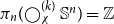 $\pi _{n}(\!\bigcirc ^{(k)}_{\chi } \mathbb{S}^{n}) = \mathbb{Z}$
.
Finally, we give some examples to illustrate that
 $\bigcirc ^{(n)} X$
can affect the homotopy groups of sufficiently high dimension.
Example 101. To illustrate that the condition of
 $\neg \neg$
-separation is necessary in Proposition 99, we give the following class of examples. Let
 $\chi : \mathbb{N} \to \nabla _{0} \mathbb{N}$
be non-computable and fix
 $k : \mathbb{N}$
. Take
 $Y_{n}$
to be the result of taking the suspension of
 $\chi (n) {\downarrow }$
 $k + 1$
times,
 $Y_{n} := \Sigma ^{k + 1} \chi (n) {\downarrow }$
. Note that each
 $Y_{n}$
is a generator of
 $\bigcirc _{\chi }^{(k + 1)}$
and so
 $\bigcirc _{\chi }^{(k + 1)}Y_{n} = 1$
, and so also
 $\pi _{k} (\!\bigcirc _{\chi }^{(k + 1)}Y_{n}) = 1$
. We can compute
 $\pi _{k}(Y_{n})$
as follows. We in fact get an explicit description of
 $\Omega ^{k}(Y_{n})$
. Recall that taking the suspension of a type is the same as taking the join with
 $2$
(Univalent Foundations Program 2013, Lemma 8.5.10). Hence, we can calculate as follows:
 \begin{align*} Y_{n} &= \Sigma ^{k + 1} \chi (n) {\downarrow } \\ &= \underbrace {2 \ast \ldots \ast 2}_{k + 1 \text{ times}} \ast \chi (n) {\downarrow } \\ &= \mathbb{S}^{k} \ast \chi (n) {\downarrow } \end{align*}
However,
 $\chi (n){\downarrow }$
is a proposition, and so
 $- \ast \chi (n){\downarrow }$
is a closed modality, which is lex (Rijke et al. Reference Rijke, Shulman and Spitters2020, Example 3.14). We deduce that
 $\Omega ^{k}(\mathbb{S}^{k} \ast \chi (n) {\downarrow }) = \Omega ^{k}(\mathbb{S}^{k}) \ast \chi (n) {\downarrow }$
, and so
 $\pi _{k} (Y_{n}) = \| \Omega ^{k}(\mathbb{S}^{k}) \ast \chi (n) {\downarrow } \|_{0}$
. Note that
 $\| \Omega ^{k}(\mathbb{S}^{k}) \ast \chi (n) {\downarrow } \|_{0}$
is modal for the closed modality
 $- \ast \chi (n){\downarrow }$
since if
 $\chi (n) {\downarrow }$
then it is contractible, and furthermore that
 $\| \Omega ^{k}(\mathbb{S}^{k}) \|_{0} \ast \chi (n) {\downarrow }$
is
 $0$
-truncated, again using that
 $- \ast \chi (n){\downarrow }$
is lex. It follows that in fact
 $\| \Omega ^{k}(\mathbb{S}^{k}) \ast \chi (n) {\downarrow } \|_{0} = \| \Omega ^{k}(\mathbb{S}^{k}) \|_{0} \ast \chi (n) {\downarrow }$
. We recall that
 $\pi _{k} \mathbb{S}^{k} = \mathbb{Z}$
, and so
 $\pi _{k}(Y_{n}) = \mathbb{Z} \ast \chi (n){\downarrow }$
. Hence from
 $\pi _{k}(\!\bigcirc _{\chi }^{(k + 1)} Y_{n}) = \pi _{k} Y_{n}$
, we could deduce
 $\chi (n) {\downarrow }$
. Therefore, when
 $\chi$
is non-computable we can show, assuming Church’s thesis, that it is false that for all
 $n$
,
 $\pi _{k}(\!\bigcirc _{\chi }^{(k + 1)}Y_{n}) = \pi _{k}(Y_{n})$
.
Example 102. The easiest example where the first homotopy group
 $\pi _{1}(X)$
is
 $\neg \neg$
-separated and altered by
 $\bigcirc ^{(1)}$
is as follows. Recall that
 $\Omega (\mathbb{S}^1) = \mathbb{Z}$
. Hence as a special case of Corollary 3.5 of Christensen et al. (Reference Christensen, Opie, Rijke and Scoccola2020), we have
 $\Omega (\!\bigcirc ^{(1)}_{\chi }(\mathbb{S}^1)) = \bigcirc _{\chi } \mathbb{Z}$
, and so
 $\pi _{1}(\!\bigcirc ^{(1)}_{\chi }(\mathbb{S}^1)) = \bigcirc _{\chi } \mathbb{Z} \neq \mathbb{Z} = \pi _{1}(\mathbb{S}^1)$
, with the inequality holding when
 $\bigcirc _{\chi }$
is non-trivial, for example, when
 $\chi$
is non-computable and Church’s thesis holds.
10. Conclusion and Future Work
We have given a new synthetic definition of Turing reducibility using modalities. We formulated the axiom of Markov induction and demonstrated its use in some synthetic proofs of Turing reducibility. Although simple, each case required an unbounded search that would not otherwise be possible. Moreover, we observe that these examples also made use of an unbounded, albeit finite, number of oracle queries. As such, we can see that the arguments in these examples would not apply to many-one reducibility or truth-table reducibility, therefore requiring the full power of Turing reducibility. We also gave an explicit proof that this definition of Turing reducibility is strictly weaker than weak truth-table reducibility in Section 4. We have also seen some first signs of interaction between computability theory and homotopy theory in Sections 8 and 9.
However, this is intended as laying the foundation for future work. We suggest a few possible directions for further research below.
10.1 Synthetic computability theory
We have developed an approach to synthetic Turing reducibility based on modalities in cubical assemblies. This was based on Hyland’s embedding of Turing degrees in the lattice of subtoposes of the effective topos but differs in a few key ways. The main difference is that working in HoTT rather than the internal logic of a topos gives us the potential to combine computability theory with higher types, with some promising signs of such interaction in Sections 8 and 9. However, even putting aside higher types, we also developed an approach that is more synthetic than Hyland’s. Instead of working externally to cubical assemblies, we identified the axioms of Markov induction and computable choice as sufficient for carrying out some simple examples of synthetic arguments, which we have formalised using the cubical Agda proof assistant. In particular, the axiom of Markov’s principle, commonly assumed in recursive constructive mathematics, is apparently insufficient for analogous arguments using computations with an oracle. In contrast, the stronger axiom of Markov induction has allowed us to show, for example, that we obtain the same class of modalities whether we only use functions
 $\mathbb{N} \to \nabla 2$
as oracles, or whether we allow all functions
 $\mathbb{N} \to \nabla \mathbb{N}$
.
10.2 Separating Turing degrees with homotopy theory
From Theorem 85, we can see that, at least in principle, it is possible to study when two Turing degrees are equal by studying homotopy groups, since oracles
 $\chi , \chi ' : \mathbb{N} \to \nabla _{0} 2$
have the same Turing degree precisely when the homotopy groups
 $\pi _{1}(\nabla \mathscr{U}, \eta (\!\bigcirc _{\chi }\!\mathbb{N}))$
and
 $\pi _{1}(\nabla \mathscr{U}, \eta (\!\bigcirc _{\chi '}\! \mathbb{N}))$
are isomorphic. We leave it for future work to determine if this is useful in practice for computability theory. However, the idea seems promising: showing that two Turing degrees are separate is a common task in computability theory, whereas in homotopy theory it is common to show two spaces are different by analysing their homotopy or (co)homology groups.
10.3 Higher-dimensional computability theory
One of the main motivations for using this formulation based on higher modalities is to make it easy to generalise computability theory to higher dimensions in order to find new interactions between computability theory and homotopy theory. We propose one such generalisation here, in a similar spirit to Kihara’s generalisations of Turing reducibility based on Lawvere–Tierney topologies in the effective topos (Kihara, Reference Kihara2022, Reference Kihara2023), which will include the examples we saw in Section 9.
Recall that we recovered the original definition of Turing degree by considering oracles of the form
 $\mathbb{N} \to \nabla _0 2$
, which leads to us nullifying only
 $\neg \neg$
-dense propositions, or in other words propositions that turn out to be simply true when we add classical logic. This is natural in computability theory: we don’t want to study the structure of the function itself, but only what we can compute with it. We therefore propose generalising the definition of Turing degree to include the nullification of countable families of
 $\nabla$
-connected types, that is, spaces that become contractible when we erase all the computational information leaving only an ordinary
 $\infty$
-groupoid. This eliminates any structure that can already be studied purely using existing techniques in homotopy theory, leaving only new structure that can only be seen through the interaction of computation and homotopy theory.
We observe that suspension preserves
 $\nabla$
-connected types, and so this does indeed include the suspension modalities of Section 9.
10.4 Automatic relativisation of proofs
As remarked in the introduction, an advantage to working with lex modalities rather than more general monads is that they correspond to reflective subuniverses, which are complete models of HoTT in themselves. This allows us to carry out any proof in HoTT internally in the reflective subuniverse to obtain a relativised version. Although this was important in formulating the theorems and definitions, and giving the intuitive ideas for the proofs, it is not used directly in the computer formalisation, which instead uses syntactic sugar, following the standard approach for working with monads in functional programming. However, this was almost entirely due to the practical difficulties involved in translating proofs by hand. Future work in this area would greatly benefit from the development of an automated approach, using Agda reflection for example.
Acknowledgements
I’m grateful for useful comments, discussions and suggestions by Mathieu Anel, Carlo Angiuli and Egbert Rijke. I also thank the anonymous referee for their helpful corrections and improvements.
Financial support
This material is based on work supported by the Air Force Office of Scientific Research under award number FA9550-21-1-0024.



