1. Introduction
The construction of the Magnetized Dusty Plasma eXperiment (MDPX) device (Thomas, Merlino & Rosenberg Reference Thomas, Merlino and Rosenberg2012, Reference Thomas, Merlino and Rosenberg2013) provides new opportunities for the examination of the orbits of charged particles in electromagnetic fields. One planned configuration has an externally imposed parabolic electrostatic potential
 $V\sim r^{2}$
combined with a uniform axial magnetic field
 $B;$
the frequency spectra of numerical calculations of the trajectories in this configuration have been examined using Fourier transforms (Bender & Thomas Reference Bender and Thomas2015). The combination of a parabolic electrostatic potential and a uniform magnetic field configuration occurs in many other contexts such as non-neutral plasmas (Davidson & Krall Reference Davidson and Krall1970; Davidson Reference Davidson1974; Dubin & O’Neil Reference Dubin and O’Neil1999) and Penning traps (Brown & Gabrielse Reference Brown and Gabrielse1986). The dusty plasma situation provides the new features that the charged particles are macroscopic, their motion can be visualized optically, the charge to mass ratio can be controlled and the electrostatic potential can be independently adjusted. The equation of motion of a charged particle in a uniform magnetic field has two normal modes, namely cyclotron motion and a zero-frequency root. When a small azimuthally symmetric electrostatic potential is added to the system these two modes change into a high-frequency mode which is a modification of the cyclotron motion and a low-frequency mode which is a modification of the zero-frequency root. The low-frequency mode is a consequence of the azimuthal
 $\boldsymbol{E}\times \boldsymbol{B}$
drift resulting from the radial electric field. However, if the electrostatic potential is large, the motion can be quite different.
In a non-neutral plasma the force resulting from the radial electric field is always radially outward but in a Penning trap this force could be inward or outward. In MDPX the force could also be either way but initial consideration has been given to an attractive (i.e. inward) force.
The orbit of a charged particle in the combination of a magnetic field and a radial force also appears in a quite different context, namely that of charged particles in accretion disks surrounding stars. Here the potential is gravitational in addition to possibly being electrostatic. The force associated with the gravitational potential is of course attractive. The author examined particle orbits in this astrophysical situation and found (Bellan Reference Bellan2007, Reference Bellan2008) that the orbits could be classified using canonical angular momentum and that the ratio of cyclotron to Kepler orbital frequency was an important parameter. An important result in Bellan (Reference Bellan2007, Reference Bellan2008) was that particles with zero canonical angular momentum would spiral in towards
 $r=0$
because these particles experienced no centrifugal force repulsion even though they had finite angular velocity. A motivation for the present work was to see if such a spiral orbit is feasible in MDPX. It turns out that this is partially possible but there is a difference because the gravitational potential scales as
 $1/r$
so a particle falls all the way down to
 $r=0$
and never comes back whereas for the parabolic potential a particle also falls down to
 $r=0$
but then bounces back out.
The first part of this paper examines and categorizes the different types of 2-D orbits possible in a parabolic potential and magnetic field. It is hoped that this will provide some useful suggestions for possible experiments on MDPX and a means for interpreting these experiments. The examination of the orbits is done from several related points of view including exact analytic solution of the equation of motion in Cartesian coordinates, consideration of canonical angular momentum, categorization of the orbits into a few different types and a correspondence to orbit stochasticity. The second part of this paper examines the related problem of the different types of orbits in the combination of a uniform magnetic field and a 3-D potential that depends on the inverse of the distance from the origin; this situation is relevant to astrophysical situations and to classical atoms in a magnetic field.
2. Exact analytic solutions
We assume an electrostatic potential
 $$\begin{eqnarray}\displaystyle V(r)=-\frac{1}{2a}E_{0}r^{2} & & \displaystyle\end{eqnarray}$$
so the electric field is
 $$\begin{eqnarray}\displaystyle \boldsymbol{E}=E_{0}\frac{\boldsymbol{r}}{a}. & & \displaystyle\end{eqnarray}$$
The equation of motion in the combination of this electric field and a uniform magnetic field
 $\boldsymbol{B}=B\hat{z}$
is (Davidson Reference Davidson1974)
 $$\begin{eqnarray}\displaystyle m\frac{\text{d}\boldsymbol{v}}{\text{d}t}=q\left(\frac{E_{0}}{a}(x\hat{x}+y{\hat{y}})+\boldsymbol{v}\times \boldsymbol{B}\right). & & \displaystyle\end{eqnarray}$$
The
 $x$
and
 $y$
components of the equation of motion are
 $$\begin{eqnarray}\displaystyle \ddot{x} & = & \displaystyle -{\it\omega}_{E}^{2}x+{\dot{y}}{\it\omega}_{c}\end{eqnarray}$$
 $$\begin{eqnarray}\displaystyle \ddot{y} & = & \displaystyle -{\it\omega}_{E}^{2}y-{\dot{x}}{\it\omega}_{c},\end{eqnarray}$$
 ${\it\omega}_{c}=qB/m$
and
 $$\begin{eqnarray}\displaystyle {\it\omega}_{E}^{2}=-\frac{qE_{0}}{ma} & & \displaystyle\end{eqnarray}$$
is positive for an attractive force and negative for a repulsive force. In the former case, the potential energy
 $qV(r)$
has the shape of a valley while in the latter case,
 $qV(r)$
has the shape of a hill. A particle is always trapped when the potential energy profile is a valley. If the potential energy is a hill, magnetic forces might keep the particle precessing around the hill at some average radius, but if the hill is sufficiently steep, the magnetic forces will be overcome and the particle will fall off the hill and go to
 $r=\infty .$
To solve (2.4) we define
 ${\it\xi}=x+\text{i}y$
and add
 $\text{i}$
times (2.4b
) to (2.4a
) to obtain
 $$\begin{eqnarray}\displaystyle \ddot{{\it\xi}}=-{\it\omega}_{E}^{2}{\it\xi}-\text{i}\dot{{\it\xi}}{\it\omega}_{c}. & & \displaystyle\end{eqnarray}$$
We assume an
 $\exp (\text{i}{\it\omega}t)$
dependence so (2.6) becomes (Davidson Reference Davidson1974)
 $$\begin{eqnarray}\displaystyle {\it\omega}^{2}+{\it\omega}{\it\omega}_{c}-{\it\omega}_{E}^{2}=0, & & \displaystyle\end{eqnarray}$$
which has the roots (Davidson Reference Davidson1974)
 $$\begin{eqnarray}\displaystyle {\it\omega}_{1} & = & \displaystyle \frac{-{\it\omega}_{c}+\sqrt{{\it\omega}_{c}^{2}+4{\it\omega}_{E}^{2}}}{2}\end{eqnarray}$$
 $$\begin{eqnarray}\displaystyle {\it\omega}_{2} & = & \displaystyle \frac{-{\it\omega}_{c}-\sqrt{{\it\omega}_{c}^{2}+4{\it\omega}_{E}^{2}}}{2}.\end{eqnarray}$$
 $q$
is negative (positive) then
 ${\it\omega}_{c}$
is negative (positive). In the case of negative
 ${\it\omega}_{c},$
 ${\it\omega}_{1}$
will be the fast frequency and
 ${\it\omega}_{2}$
will be the slow frequency while in the case of positive
 ${\it\omega}_{c},$
 ${\it\omega}_{2}$
will be the fast frequency and
 ${\it\omega}_{1}$
will be the slow frequency. Because dust grains in MDPX are negatively charged we will assume
 ${\it\omega}_{c}$
is negative so
 ${\it\omega}_{1}$
will be the fast frequency and
 ${\it\omega}_{2}$
will be the slow frequency. Also, if the potential is valley-like (attractive) then
 $qE_{0}<0$
so
 ${\it\omega}_{E}^{2}$
is positive and (2.8) shows that
 ${\it\omega}_{1,2}$
are always real. However, if the potential is hill-like (repulsive) then
 ${\it\omega}_{E}^{2}$
is negative and
 ${\it\omega}_{1,2}$
are real only if
 ${\it\omega}_{c}^{2}>4|{\it\omega}_{E}^{2}|$
which corresponds to the Brillouin limit.
The general solution to (2.6) is
 $$\begin{eqnarray}\displaystyle {\it\xi}={\it\alpha}\text{e}^{\text{i}{\it\omega}_{1}t}+{\it\beta}\text{e}^{\text{i}{\it\omega}_{2}t}, & & \displaystyle\end{eqnarray}$$
where
 ${\it\alpha}$
and
 ${\it\beta}$
are determined by the initial conditions. The derivative of (2.9) is
 $$\begin{eqnarray}\displaystyle \dot{{\it\xi}}=\text{i}{\it\omega}_{1}{\it\alpha}\text{e}^{\text{i}{\it\omega}_{1}t}+\text{i}{\it\omega}_{2}{\it\beta}\text{e}^{\text{i}{\it\omega}_{2}t}. & & \displaystyle\end{eqnarray}$$
The initial conditions on position and velocity give
 $$\begin{eqnarray}\displaystyle x_{0}+\text{i}y_{0} & = & \displaystyle {\it\alpha}+{\it\beta}\end{eqnarray}$$
 $$\begin{eqnarray}\displaystyle v_{x0}+\text{i}v_{y0} & = & \displaystyle \text{i}{\it\omega}_{1}{\it\alpha}+\text{i}{\it\omega}_{2}{\it\beta},\end{eqnarray}$$
 $x_{0},y_{0}$
are the position at
 $t=0$
and
 $v_{x0},v_{y0}$
are the velocity at
 $t=0$
. Equations (2.11) constitute two coupled algebraic equations in the unknowns
 ${\it\alpha},{\it\beta}$
which can be solved to give
 $$\begin{eqnarray}\displaystyle {\it\alpha} & = & \displaystyle -\frac{{\it\omega}_{2}x_{0}-v_{y0}+\text{i}({\it\omega}_{2}y_{0}+v_{x0})}{\sqrt{{\it\omega}_{c}^{2}+4{\it\omega}_{E}^{2}}}\end{eqnarray}$$
 $$\begin{eqnarray}\displaystyle {\it\beta} & = & \displaystyle \frac{{\it\omega}_{1}x_{0}-v_{y0}+\text{i}({\it\omega}_{1}y_{0}+v_{x0})}{\sqrt{{\it\omega}_{c}^{2}+4{\it\omega}_{E}^{2}}}.\end{eqnarray}$$
We can decompose
 ${\it\alpha}$
and
 ${\it\beta}$
into real and imaginary parts so
 ${\it\alpha}={\it\alpha}_{r}+\text{i}{\it\alpha}_{i},{\it\beta}={\it\beta}_{r}+\text{i}{\it\beta}_{i}$
where
 $$\begin{eqnarray}\displaystyle {\it\alpha}_{r} & = & \displaystyle -\frac{{\it\omega}_{2}x_{0}-v_{y0}}{\sqrt{{\it\omega}_{c}^{2}+4{\it\omega}_{E}^{2}}}\end{eqnarray}$$
 $$\begin{eqnarray}\displaystyle {\it\alpha}_{i} & = & \displaystyle -\frac{{\it\omega}_{2}y_{0}+v_{x0}}{\sqrt{{\it\omega}_{c}^{2}+4{\it\omega}_{E}^{2}}}\end{eqnarray}$$
 $$\begin{eqnarray}\displaystyle {\it\beta}_{r} & = & \displaystyle \frac{{\it\omega}_{1}x_{0}-v_{y0}}{\sqrt{{\it\omega}_{c}^{2}+4{\it\omega}_{E}^{2}}}\end{eqnarray}$$
 $$\begin{eqnarray}\displaystyle {\it\beta}_{i} & = & \displaystyle \frac{{\it\omega}_{1}y_{0}+v_{x0}}{\sqrt{{\it\omega}_{c}^{2}+4{\it\omega}_{E}^{2}}}.\end{eqnarray}$$
 $$\begin{eqnarray}\displaystyle x+\text{i}y=({\it\alpha}_{r}+\text{i}{\it\alpha}_{i})\text{e}^{\text{i}{\it\omega}_{1}t}+({\it\beta}_{r}+\text{i}{\it\beta}_{i})\text{e}^{\text{i}{\it\omega}_{2}t} & & \displaystyle\end{eqnarray}$$
and its complex conjugate can be written as
 $$\begin{eqnarray}\displaystyle x-\text{i}y=({\it\alpha}_{r}-\text{i}{\it\alpha}_{i})\text{e}^{-\text{i}{\it\omega}_{1}t}+({\it\beta}_{r}-\text{i}{\it\beta}_{i})\text{e}^{-\text{i}{\it\omega}_{2}t}. & & \displaystyle\end{eqnarray}$$
Adding (2.15) and (2.16) gives
 $$\begin{eqnarray}\displaystyle x(t)={\it\alpha}_{r}\cos ({\it\omega}_{1}t)-{\it\alpha}_{i}\sin ({\it\omega}_{1}t)+{\it\beta}_{r}\cos ({\it\omega}_{2}t)-{\it\beta}_{i}\sin ({\it\omega}_{2}t) & & \displaystyle\end{eqnarray}$$
while subtracting (2.16) from (2.15) gives
 $$\begin{eqnarray}\displaystyle y(t)={\it\alpha}_{r}\sin ({\it\omega}_{1}t)+{\it\alpha}_{i}\cos ({\it\omega}_{1}t)+{\it\beta}_{r}\sin ({\it\omega}_{2}t)+{\it\beta}_{i}\cos ({\it\omega}_{2}t). & & \displaystyle\end{eqnarray}$$
Equations (2.17) and (2.18) give the exact analytic solutions to (2.3) with specified initial conditions
 $x_{0},y_{0},v_{x0},v_{y0}$
determining the coefficients
 ${\it\alpha}_{r},{\it\alpha}_{i},$
 ${\it\beta}_{r},{\it\beta}_{i}$
using equations (2.13) and (2.14) and equation (2.8) determining
 ${\it\omega}_{1}$
and
 ${\it\omega}_{2}$
. Equations (2.17) and (2.18) are exact and so are useful for plotting, comparison to numerical solutions and comparison to experiment.
Equations (2.17) and (2.18) also provide the following important insight. We had assumed that
 ${\it\omega}_{1}$
is the fast frequency and so suppose that (2.17) and (2.18) are averaged over this fast frequency. Such an averaging will annihilate the terms involving
 $\sin ({\it\omega}_{1}t)$
and
 $\cos ({\it\omega}_{1}t)$
but retain the terms involving
 $\sin ({\it\omega}_{2}t)$
and
 $\cos ({\it\omega}_{2}t)$
. In this case, (2.15) can be written as
 $$\begin{eqnarray}\displaystyle \langle x\rangle +\text{i}\langle y\rangle =({\it\beta}_{r}+\text{i}{\it\beta}_{i})\text{e}^{\text{i}{\it\omega}_{2}t}, & & \displaystyle\end{eqnarray}$$
where the angle brackets denote averaging over the fast frequency. We may then write
 $$\begin{eqnarray}\displaystyle \langle x\rangle +\text{i}\langle y\rangle =\langle r\rangle \text{e}^{\text{i}\langle {\it\phi}\rangle }, & & \displaystyle\end{eqnarray}$$
where
 $\langle r\rangle$
and
 $\langle {\it\phi}\rangle$
are quantities also averaged over the fast frequency. Combining (2.19) and (2.20) shows that
 $$\begin{eqnarray}\displaystyle \langle r\rangle \text{e}^{\text{i}\langle {\it\phi}\rangle }=({\it\beta}_{r}+\text{i}{\it\beta}_{i})\text{e}^{\text{i}{\it\omega}_{2}t} & & \displaystyle\end{eqnarray}$$
so that the average radius is
 $$\begin{eqnarray}\displaystyle \langle r\rangle =\sqrt{{\it\beta}_{r}^{2}+{\it\beta}_{i}^{2}} & & \displaystyle\end{eqnarray}$$
and the average angular velocity is given by
 $\dot{{\it\phi}}={\it\omega}_{2}.$
3. Guiding centre approximation
The guiding centre approximation (GCA) assumes an ordering such that the cyclotron frequency is much larger than other frequencies of the system. This corresponds to assuming that
 ${\it\omega}_{c}^{2}\gg 4{\it\omega}_{2}^{2}$
so that Taylor expansion gives
 $\sqrt{{\it\omega}_{c}^{2}+4{\it\omega}_{E}^{2}}\simeq |{\it\omega}_{c}|+2{\it\omega}_{E}^{2}/|{\it\omega}_{c}|.$
If
 $q$
is positive, then (2.8) reduce in this limit to
 ${\it\omega}_{1}\simeq {\it\omega}_{E}^{2}/{\it\omega}_{c}=-E_{0}/(aB)$
and
 ${\it\omega}_{2}=-{\it\omega}_{c}.$
If
 $q$
is negative, then (2.8) reduce to
 ${\it\omega}_{2}\simeq {\it\omega}_{E}^{2}/{\it\omega}_{c}=-E_{0}/(aB)$
and
 ${\it\omega}_{1}=-{\it\omega}_{c}.$
The solutions where
 ${\it\omega}_{1,2}=-E_{0}/(aB)$
are just the angular velocities associated with a generalization of the
 $\boldsymbol{E}\times \boldsymbol{B}$
drift since
 $\boldsymbol{v}_{E}=\boldsymbol{E}\times \boldsymbol{B}/B^{2}=E_{0}\hat{r}\times B\hat{z}/B^{2}=-E_{0}\hat{{\it\phi}}/B$
gives
 $\dot{{\it\phi}}=-E_{0}/(aB)$
at
 $r=a$
. It must be emphasized that the GCA depends on making a Taylor expansion presuming
 ${\it\omega}_{c}^{2}\gg 4{\it\omega}_{E}^{2}$
so the GCA fails when this assumption is untrue. Thus the entire GCA hierarchy (cyclotron orbit,
 $\boldsymbol{E}\times \boldsymbol{B}$
drift, polarization drift, grad
 $B$
drift, curvature drift) becomes incorrect if
 ${\it\omega}_{c}^{2}\gg 4{\it\omega}_{E}^{2}$
is not valid.
4. Vector point of view
Equations (2.17) and (2.18) can be recast as
 $$\begin{eqnarray}\displaystyle \boldsymbol{r}(t)=\boldsymbol{r}_{1}(t)+\boldsymbol{r}_{2}(t), & & \displaystyle\end{eqnarray}$$
where
 $$\begin{eqnarray}\displaystyle \boldsymbol{r}_{1}(t) & = & \displaystyle C_{1}[\hat{x}\cos ({\it\omega}_{1}t+{\it\delta}_{1})+{\hat{y}}\sin ({\it\omega}_{1}t+{\it\delta}_{1})]\end{eqnarray}$$
 $$\begin{eqnarray}\displaystyle \boldsymbol{r}_{2}(t) & = & \displaystyle C_{2}[\hat{x}\cos ({\it\omega}_{2}t+{\it\delta}_{2})+{\hat{y}}\sin ({\it\omega}_{2}t+{\it\delta}_{2})]\end{eqnarray}$$
 $$\begin{eqnarray}\displaystyle C_{1} & = & \displaystyle \sqrt{{\it\alpha}_{r}^{2}+{\it\alpha}_{i}^{2}}\end{eqnarray}$$
 $$\begin{eqnarray}\displaystyle C_{2} & = & \displaystyle \sqrt{{\it\beta}_{r}^{2}+{\it\beta}_{i}^{2}}\end{eqnarray}$$
 $$\begin{eqnarray}\displaystyle {\it\delta}_{1} & = & \displaystyle \tan ^{-1}\left(\frac{{\it\alpha}_{i}}{{\it\alpha}_{r}}\right)\end{eqnarray}$$
 $$\begin{eqnarray}\displaystyle {\it\delta}_{2} & = & \displaystyle \tan ^{-1}\left(\frac{{\it\beta}_{i}}{{\it\beta}_{r}}\right).\end{eqnarray}$$
 $\boldsymbol{r}_{1}(t)$
is a vector of length
 $C_{1}$
rotating with angular velocity
 ${\it\omega}_{1}$
while
 $\boldsymbol{r}_{2}(t)$
is a vector of length
 $C_{2}$
rotating with angular velocity
 ${\it\omega}_{2}$
and
 $\boldsymbol{r}(t)$
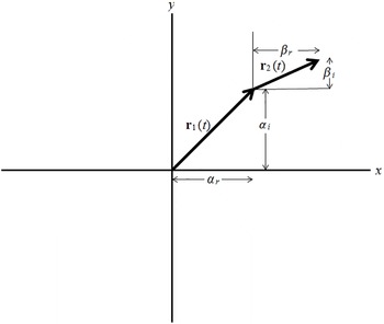
is the sum of these two vectors. This is shown in figure 1. At
 $t=0$
the horizontal component of
 $\boldsymbol{r}_{1}(t)$
is
 ${\it\alpha}_{r}$
and the vertical component is
 ${\it\alpha}_{i}$
while the horizontal component of
 $\boldsymbol{r}_{2}(t)$
is
 ${\it\beta}_{r}$
and the vertical component is
 ${\it\beta}_{i}$
. The orbits will be closed if
 $N_{1}{\it\omega}_{1}=N_{2}{\it\omega}_{2}$
where
 $N_{1}$
and
 $N_{2}$
are integers.
The particle position
 $\boldsymbol{r}$
is the sum of
 $\boldsymbol{r}_{1}(t)$
and
 $\boldsymbol{r}_{2}(t)$
rotating at respective angular velocities
 ${\it\omega}_{1}$
and
 ${\it\omega}_{2}$
. These vectors are shown at time
 $t=0$
.

The GCA corresponds to the
 $\boldsymbol{r}_{1}(t)$
vector being much longer than the
 $\boldsymbol{r}_{2}(t)$
vector and rotating much more slowly than the
 $\boldsymbol{r}_{2}(t)$
vector; these orbits are non-axis-encircling and this could happen if
 ${\it\omega}_{1}$
is the slow frequency. The situation where
 $\boldsymbol{r}_{1}(t)$
vector is much shorter than the
 $\boldsymbol{r}_{2}(t)$
vector gives axis-encircling orbits and in the limit that
 $C_{1}=0,$
the orbits are circular at frequency
 ${\it\omega}_{2}.$
Similarly, in the situation where
 $C_{2}=0$
, the orbits are circular at frequency
 ${\it\omega}_{1}.$
Situations of either
 $C_{1}=0$
or
 $C_{2}=0$
can be established by appropriate choice of the initial conditions
 $x_{0},y_{0},v_{x0},$
and
 $v_{y0}$
in (2.13) and (2.14). For example, choosing
 $v_{y0}/x_{0}={\it\omega}_{2}$
and
 $v_{x0}/y_{0}=-{\it\omega}_{2}$
will set
 ${\it\alpha}_{r}={\it\alpha}_{i}=0$
and so give
 $C_{1}=0.$
Equations (4.2) are related to the rotating-frame solutions given by equation (1.2.12) in Davidson (Reference Davidson1974) but differ because each of (4.2) gives the rotation of a vector in laboratory-frame coordinates, whereas equation (1.2.12) in Davidson (Reference Davidson1974) is given in a frame rotating with angular velocity
 ${\it\omega}_{1}$
or
 ${\it\omega}_{2}$
and in this rotating frame, the particle rotates with an angular velocity given by
 $|{\it\omega}_{1}-{\it\omega}_{2}|$
.
5. Relation to stochastic orbits in electrostatic waves and the Brillouin limit of non-neutral plasmas
McChesney, Stern & Bellan (Reference McChesney, Stern and Bellan1987) observed rapid collisionless heating of ions by coherent drift waves in a small tokamak and showed that this resulted from a stochastic mechanism. This collisionless mechanism has since been proposed as an explanation for transport in tokamaks (Bellan Reference Bellan1993), for collisionless heating in the solar corona (Vranjes & Poedts Reference Vranjes and Poedts2010), for collisionless ion heating by Alfvén waves (Chandran et al. Reference Chandran, Verscharen, Quataert, Kasper, Isenberg and Bourouaine2013) and for collisionless turbulent heating of ions when the solar wind forms a bow shock as it collides with the Earth’s magnetosphere (Stasiewicz et al. Reference Stasiewicz, Markidis, Eliasson, Strumik and Yamauchi2013).
The essence of this stochastic mechanism is that the GCA fails when the wave amplitude becomes sufficiently large that the excursion a particle makes due to polarization drift can no longer be considered small compared to a wavelength. When this failure occurs, the particle motion can no longer be characterized as the sum of an
 $\boldsymbol{E}\times \boldsymbol{B}$
drift, a polarization drift and the various other guiding centre drifts.
The polarization drift is given by
 $\boldsymbol{v}_{p}=m\dot{\boldsymbol{E}}_{\bot }/(qB^{2})$
so if the wave is electrostatic then the polarization drift is
 $\boldsymbol{v}_{p}=\text{i}{\it\omega}m(-\text{i}\boldsymbol{k}_{\bot }\tilde{{\it\phi}})/(qB^{2})$
where
 $\tilde{{\it\phi}}$
is the wave electrostatic potential. The displacement made by a particle undergoing this polarization drift is
 ${\it\delta}\boldsymbol{x}=\int \boldsymbol{v}_{p}\,\text{d}t=-\text{i}\boldsymbol{k}_{\bot }\tilde{{\it\phi}}m/(qB^{2})$
and the displacement will be of the order of a quarter wavelength if
 $\boldsymbol{k}\boldsymbol{\cdot }{\it\delta}\boldsymbol{x}\simeq {\rm\pi}/2.$
Since the wave phase will be completely different from that assumed in the GCA when this happens, a necessary condition for the GCA to work is
 $$\begin{eqnarray}\displaystyle \frac{k_{\bot }^{2}\tilde{{\it\phi}}m}{qB^{2}}\ll {\rm\pi}/2. & & \displaystyle\end{eqnarray}$$
Now consider (2.8a
) and (2.8b
). If
 ${\it\omega}_{E}^{2}$
is negative then the potential is hill-type and if this is the case and
 $$\begin{eqnarray}\displaystyle \frac{|{\it\omega}_{E}^{2}|}{{\it\omega}_{c}^{2}}>\frac{1}{4} & & \displaystyle\end{eqnarray}$$
then one of (2.8a
) and (2.8b
) provides an unstable, exponentially growing solution. Using (2.5), assuming
 $k\sim 1/a,$
and using
 $E\simeq \tilde{{\it\phi}}/a=k\tilde{{\it\phi}}$
it is seen that (5.2) corresponds to
 $$\begin{eqnarray}\displaystyle \frac{k^{2}q\tilde{{\it\phi}}}{m\left({\displaystyle \frac{q^{2}B^{2}}{m^{2}}}\right)}>\frac{1}{4}, & & \displaystyle\end{eqnarray}$$
which corresponds to violating (5.1).
The orbit will always be closed at the transition to instability because (i) at the transition to instability
 ${\it\omega}_{c}^{2}+4{\it\omega}_{E}^{2}=0$
so (2.8a,b
) give
 ${\it\omega}_{1}={\it\omega}_{2}$
and (ii) the discussion after (4.3d
) shows that orbits are closed if
 $N_{1}{\it\omega}_{1}=N_{2}{\it\omega}_{2}$
where
 $N_{1}$
and
 $N_{2}$
are integers. Thus, the transition to instability involves a closed orbit with
 $N_{1}=N_{2}=1.$
As discussed in Bellan (Reference Bellan1993), drift wave turbulence can be considered to be a collection of random potential hills and valleys. If (5.3) is not satisfied, then particles forever remain on their respective initial hills or valleys. However, if (5.3) is satisfied, then a particle initially on a hill will fall off of this hill into an adjacent valley, bounce out of the valley in some random direction and climb up some other adjacent hill. The particle will then wander chaotically over the entire system of hills and valleys. Thus, (5.3) is the condition for particles in a turbulent electrostatic electric field to have chaotic trajectories that cover all of the
 $x$
–
 $y$
plane. By subtracting the Lorentz equations characterizing the motion of two adjacent particles, Stasiewicz, Lundin & Marklund (Reference Stasiewicz, Lundin and Marklund2000) showed that (5.3) corresponds to the two particles having exponentially diverging trajectories.
Equation (5.2) is also related to the Brillouin limit of a non-neutral plasma. If the density of this plasma is
 $n$
and its radius is
 $a$
then Poisson’s equation gives
 $E_{r}=anq/(2{\it\varepsilon}_{0})$
and the potential is hill-type because the like-sign particles repel each other. Using (2.5) with this self-electric field, the condition for single-particle orbit instability given by (5.2) becomes
 $$\begin{eqnarray}\displaystyle n>\frac{2B^{2}}{{\it\mu}_{0}mc^{2}}, & & \displaystyle\end{eqnarray}$$
which, except for a numerical factor, is identical to the Brillouin limit condition for instability of a rigidly rotating uniform-density non-neutral plasma.
6. Hamiltonian point of view
The vector potential is
 $\boldsymbol{A}=A_{{\it\phi}}\hat{{\it\phi}}=Br\hat{{\it\phi}}/2$
and the Lagrangian for this system can be expressed in cylindrical coordinates as
 $$\begin{eqnarray}\displaystyle L={\textstyle \frac{1}{2}}mv_{r}^{2}+{\textstyle \frac{1}{2}}mr^{2}\dot{{\it\phi}}^{2}+qr\dot{{\it\phi}}A_{{\it\phi}}+qV(r). & & \displaystyle\end{eqnarray}$$
The canonical angular momentum is
 $$\begin{eqnarray}\displaystyle P_{{\it\phi}}=\frac{\partial L}{\partial \dot{{\it\phi}}}=mr^{2}\dot{{\it\phi}}+qrA_{{\it\phi}} & & \displaystyle\end{eqnarray}$$
so
 $$\begin{eqnarray}\displaystyle \dot{{\it\phi}}=\frac{P_{{\it\phi}}-qBr^{2}/2}{mr^{2}}. & & \displaystyle\end{eqnarray}$$
The Hamiltonian is, using (2.1)
 $$\begin{eqnarray}\displaystyle H=\frac{P_{r}^{2}}{2m}+\bbox[border:1px solid black]{\text{}{\displaystyle \frac{(P_{{\it\phi}}-qBr^{2}/2)^{2}}{2mr^{2}}}\text{}}-\frac{1}{2a}qE_{0}r^{2}. & & \displaystyle\end{eqnarray}$$
As discussed in Schmidt (Reference Schmidt1979) and in Bellan (Reference Bellan2006) there are two general types of orbits, axis-encircling and non-axis-encircling. For axis-encircling orbits the sign of
 $\dot{{\it\phi}}$
never changes whereas for non-axis-encircling orbits the sign of
 $\dot{{\it\phi}}$
oscillates between being positive and negative. Examination of (6.3) shows that axis-encircling orbits occur when
 $P_{{\it\phi}}$
has the opposite sign of
 $qB$
whereas non-axis-encircling orbits occur if
 $P_{{\it\phi}}$
has the same sign as
 $qB$
, in which case
 $r$
oscillates about the position where
 $P_{{\it\phi}}=qBr^{2}/2.$
The transition between axis-encircling and non-axis-encircling orbits thus corresponds to the special situation where
 $P_{{\it\phi}}=0.$
The
 $P_{{\it\phi}}=0$
situation corresponds to the length of the
 $\boldsymbol{r}_{1}(t)$
vector discussed in § 4 being equal to the length of the
 $\boldsymbol{r}_{2}(t)$
vector making it possible to have
 $\boldsymbol{r}_{1}(t)+\boldsymbol{r}_{2}(t)=0$
, in which case the particle passes through the origin. This
 $P_{{\it\phi}}=0$
situation is thus very different from the GCA where the motion can be decomposed into cyclotron motion and an
 $\boldsymbol{E}\times \boldsymbol{B}$
drift.
If
 $P_{{\it\phi}}=0$
in (6.4), both the electrostatic potential and the generalization of the centrifugal potential (i.e. boxed term in (6.4)) scale as
 $r^{2}.$
If
 $qE_{0}<0$
these two terms are additive so the net potential is valley-like in which case the particle bounces through
 $r=0$
. If
 $qE_{0}>0$
, corresponding to a repulsive electric force, the particle will bounce about
 $r=0$
if
 $q^{2}B^{2}/m>4qE_{0}/a$
but if
 $q^{2}B^{2}/m<4qE_{0}/a$
the particle will be on a potential hill and will fall outwards towards
 $r=\infty .$
Equation (6.3) shows that a particle with
 $P_{{\it\phi}}=0$
will have an angular velocity
 $\dot{{\it\phi}}=-qB/(2m)=-{\it\omega}_{c}/2$
independent of
 $r$
. Thus
 $P_{{\it\phi}}=0$
particles in valley-like potentials will bounce back and forth through
 $r=0$
while simultaneously having
 $\dot{{\it\phi}}=-{\it\omega}_{c}/2$
whereas particles for which
 $q^{2}B^{2}/m<4qE_{0}/a$
will spiral out towards
 $r=\infty$
also with an angular velocity
 $\dot{{\it\phi}}=-{\it\omega}_{c}/2$
independent of
 $r$
. The bouncing through
 $r=0$
of
 $P_{{\it\phi}}=0$
particles in valley-like potentials provides a focusing mechanism slightly analogous to that proposed for inertial electrostatic fusion (Elmore, Tuck & Watson Reference Elmore, Tuck and Watson1959; Hirsch Reference Hirsch1967).
The canonical angular momentum can be written in Cartesian coordinates as
 $$\begin{eqnarray}\displaystyle P_{{\it\phi}}=m(xv_{y}-yv_{x})+{\textstyle \frac{1}{2}}qB(x^{2}+y^{2}) & & \displaystyle\end{eqnarray}$$
and since
 $P_{{\it\phi}}$
is a constant of the motion, it can be evaluated from the initial conditions so
 $$\begin{eqnarray}\displaystyle P_{{\it\phi}}=m(x_{0}v_{y0}-y_{0}v_{x0})+{\textstyle \frac{1}{2}}qB(x_{0}^{2}+y_{0}^{2}). & & \displaystyle\end{eqnarray}$$
One can always rotate the coordinate system so that
 $y_{0}=0$
and
 $x_{0}$
is positive in which case
 $$\begin{eqnarray}\displaystyle P_{{\it\phi}}=\left(v_{y0}+{\textstyle \frac{1}{2}}{\it\omega}_{c}x_{0}\right)mx_{0} & & \displaystyle\end{eqnarray}$$
so
 $P_{{\it\phi}}=0$
corresponds in this rotated coordinate system to choosing
 $v_{y0}=-qBx_{0}/(2m)$
with the value of
 $v_{x0}$
being arbitrary. This corresponds to having
 $C_{1}=C_{2}$
in (4.2).
If
 $P_{{\it\phi}}\neq 0$
and
 $qB>0$
then
 $P_{{\it\phi}}$
will be positive if
 $qBx_{0}/(2m)>-v_{y0}$
in which case
 $qB$
will have the same sign as
 $P_{{\it\phi}}$
and the particle will be non-axis-encircling. The particle will be axis-encircling if
 $qBx_{0}/(2m)<-v_{y0}.$
These conditions for axis- and non-axis-circling orbits will reverse if
 $qB<0.$
Equation (6.7) can be written as
 $$\begin{eqnarray}\displaystyle \frac{P_{{\it\phi}}}{m{\it\omega}_{c}x_{0}^{2}}=\frac{v_{y0}}{{\it\omega}_{c}x_{0}}+\frac{1}{2}. & & \displaystyle\end{eqnarray}$$
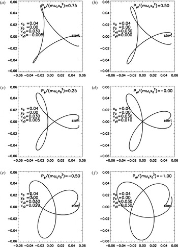
Figure 2 plots trajectories for a sequence of values of
 $P_{{\it\phi}}/(m{\it\omega}_{c}x_{0}^{2})$
for a negatively charged dust particle with parameters relevant to MDPX and shows the transition from non-axis-encircling (positive
 $P_{{\it\phi}}$
) to axis-encircling (negative
 $P_{{\it\phi}}$
) and also that particles with
 $P_{{\it\phi}}=0$
have trajectories that go through the origin.
Trajectories from (2.17) and (2.18) for particles with charge
 $q=-112.492e,$
radius
 $0.25~{\rm\mu}\text{m}$
, mass density
 ${\it\rho}=2200~\text{kg}~\text{m}^{-3}$
in
 $B=4$
T magnetic field starting from
 $x_{0}=0.04$
m,
 $y_{0}=0.0$
m with velocity
 $v_{x0}=0.03~\text{m}~\text{s}^{-1}$
. The initial
 $v_{y0}$
differs in each plot and is given in the plots, as is
 $P_{{\it\phi}}/(m{\it\omega}_{c}x_{0}^{2}).$
The trajectories are non-axis-encircling for (a–c) corresponding to positive
 $P_{{\it\phi}}$
. The trajectory goes through the origin for (d) which has
 $P_{{\it\phi}}=0$
. The trajectories are axis-encircling for (e) and (f) which have
 $P_{{\it\phi}}<0$
.

7. Action integral point of view
The action integral for radial motion is
 $$\begin{eqnarray}\displaystyle J=\oint P_{r}\,\text{d}r, & & \displaystyle\end{eqnarray}$$
where the integration is over one complete cycle of radial oscillation. The radial momentum
 $P_{r}$
is solved for using (6.4) to obtain
 $$\begin{eqnarray}\displaystyle P_{r}=\sqrt{2mH-\frac{(P_{{\it\phi}}-qBr^{2}/2)^{2}}{r^{2}}+\frac{mqE_{0}}{a}r^{2}} & & \displaystyle\end{eqnarray}$$
and so using (2.5) the action can be expressed as
 $$\begin{eqnarray}\displaystyle J=m\oint \sqrt{\frac{2H}{m}+\frac{P_{{\it\phi}}}{m}{\it\omega}_{c}-\frac{P_{{\it\phi}}^{2}}{m^{2}r^{2}}-\left({\it\omega}_{E}^{2}+\frac{{\it\omega}_{c}^{2}}{4}\right)r^{2}}\,\text{d}r. & & \displaystyle\end{eqnarray}$$
As shown in appendix A of Perkins & Bellan (Reference Perkins and Bellan2015) the integral in (7.3) can be evaluated to give
 $$\begin{eqnarray}\displaystyle J=-{\rm\pi}|P_{{\it\phi}}|+2{\rm\pi}\frac{H+{\it\omega}_{c}P_{{\it\phi}}/2}{\sqrt{{\it\omega}_{c}^{2}+4{\it\omega}_{E}^{2}}}. & & \displaystyle\end{eqnarray}$$
Perkins & Bellan (Reference Perkins and Bellan2010) showed that the period
 ${\rm\Delta}t$
of the radial oscillation is given by
 $$\begin{eqnarray}\displaystyle {\rm\Delta}t=\frac{\partial J}{\partial H}=\frac{2{\rm\pi}}{\sqrt{{\it\omega}_{c}^{2}+4{\it\omega}_{E}^{2}}} & & \displaystyle\end{eqnarray}$$
and that the increment in
 ${\it\phi}$
during one radial oscillation is given by
 $$\begin{eqnarray}\displaystyle {\rm\Delta}{\it\phi}=-\frac{\partial J}{\partial P_{{\it\phi}}}. & & \displaystyle\end{eqnarray}$$
Because of the absolute value sign in (7.4) it is necessary to make separate evaluations of (7.6) for positive and negative
 $P_{{\it\phi}}.$
If
 $P_{{\it\phi}}$
is positive then
 $$\begin{eqnarray}\displaystyle J=-{\rm\pi}P_{{\it\phi}}+2{\rm\pi}\frac{H+{\it\omega}_{c}P_{{\it\phi}}/2}{\sqrt{{\it\omega}_{c}^{2}+4{\it\omega}_{E}^{2}}} & & \displaystyle\end{eqnarray}$$
and
 $$\begin{eqnarray}\displaystyle {\rm\Delta}{\it\phi}={\rm\pi}-{\rm\pi}\frac{{\it\omega}_{c}}{\sqrt{{\it\omega}_{c}^{2}+4{\it\omega}_{E}^{2}}}. & & \displaystyle\end{eqnarray}$$
The
 ${\it\phi}$
drift velocity is using (7.8) and (7.5) is
 $$\begin{eqnarray}\displaystyle \frac{{\rm\Delta}{\it\phi}}{{\rm\Delta}t}=\frac{\sqrt{{\it\omega}_{c}^{2}+4{\it\omega}_{E}^{2}}}{2}-\frac{{\it\omega}_{c}}{2}, & & \displaystyle\end{eqnarray}$$
which is just
 ${\it\omega}_{1}$
as given by (2.8a
). If
 $P_{{\it\phi}}$
is negative then the same procedure will give the
 ${\it\phi}$
drift velocity to be
 ${\it\omega}_{2}.$
8. Extension of the Hamiltonian point of view to 3-D and gravitational and atomic potentials
In three dimensions the electrostatic potential of a spherical source of spherical radius
 $a$
is
 $$\begin{eqnarray}\displaystyle V(r,z)=\frac{Q}{4{\rm\pi}{\it\varepsilon}_{0}\sqrt{r^{2}+z^{2}}} & & \displaystyle\end{eqnarray}$$
for
 $r^{2}+z^{2}>a^{2}$
and where
 $r^{2}=x^{2}+y^{2}.$
In the limit
 $a\rightarrow 0,$
the source may be considered a point source, but here we will consider
 $a$
small but finite and will assume that if a charged particle coming from large
 $r,z$
impacts the source it will be absorbed. Such a situation is relevant to a spherical Langmuir probe collecting charged particles or a spherical dust grain collecting charged particles. In both these cases, the charge on the sphere is related to the potential at the surface of the sphere by
 $V_{sfc}=Q/(4{\rm\pi}{\it\varepsilon}_{0}a).$
Noting that
 $v_{{\it\phi}}=r\dot{{\it\phi}}$
and using (6.3), the Hamiltonian for this 3-D situation is
 $$\begin{eqnarray}\displaystyle H=\frac{P_{r}^{2}}{2m}+\bbox[border:1px solid black]{\text{}{\displaystyle \frac{(P_{{\it\phi}}-qBr^{2}/2)^{2}}{2mr^{2}}}\text{}}+\frac{P_{z}^{2}}{2m}+\frac{qQ}{4{\rm\pi}{\it\varepsilon}_{0}\sqrt{r^{2}+z^{2}}}. & & \displaystyle\end{eqnarray}$$
This situation is also relevant to a hydrogen or anti-hydrogen atom in a uniform magnetic field such as has been previously modelled by Vrinceanu et al. (Reference Vrinceanu, Granger, Parrott, Sadeghpour, Cederbaum, Mody, Tan and Gabrielse2004) and by Kuzmin & O’Neil (Reference Kuzmin and O’Neil2005). We note that these previous models used a Cartesian coordinate system and failed to take into account that
 $P_{{\it\phi}}$
is a constant of the motion; in particular these previous models expressed the kinetic energy as
 $[P_{x}^{2}+(P_{y}-qA_{y})^{2}+P_{z}^{2}]/(2m)$
where none of
 $P_{x},$
 $P_{y}$
or
 $P_{z}$
is a constant of the motion. A mathematically identical situation to (8.2) occurs for the gravitational potential of a mass
 $M$
central object where the Hamiltonian has the form
 $$\begin{eqnarray}\displaystyle H=\frac{P_{r}^{2}}{2m}+\bbox[border:1px solid black]{\text{}{\displaystyle \frac{(P_{{\it\phi}}-qBr^{2}/2)^{2}}{2mr^{2}}}\text{}}+\frac{P_{z}^{2}}{2m}-\frac{mMG}{\sqrt{r^{2}+z^{2}}}. & & \displaystyle\end{eqnarray}$$
Comparison of (8.2) and (8.3) shows that the atomic and the gravitational situations can be mapped to each other using
 $qQ/(4{\rm\pi}{\it\varepsilon}_{0})\Leftrightarrow -mMG.$
If
 $qQ<0$
(attractive potential) the atomic situation is mathematically identical to the gravitational situation. This is the classical limit of hydrogen and anti-hydrogen atoms.
The boxed terms on the right-hand sides of (8.2) and (8.3) generalize the centrifugal potential. If
 $B=0$
, these boxed terms reduce to
 $P_{{\it\phi}}^{2}/(2mr^{2})$
and the gravitational Hamiltonian describes Kepler orbits, i.e. situations where the outward centrifugal force is balanced by the inward gravitational force. In the atomic case, these would be classical Bohr orbits. However, if
 $P_{{\it\phi}}=0$
, then the boxed terms become
 $q^{2}B^{2}r^{2}/(8m)$
and so constitute an attractive or valley-like potential providing a force towards the
 $z$
axis. The gravitational or Bohr atom potential correspond to an attractive force pushing the particle towards the origin (i.e. where both
 $r=0$
and
 $z=0$
) so the boxed terms and the potential term combine to give a net attractive force towards the origin, i.e. towards the central object responsible for the gravitational force or towards the nucleus in the case of an atom. The particle falls in towards
 $r=0,$
 $z=0$
never to come back because the gravitational potential energy is
 $-\infty$
at
 $r=0$
. If
 $P_{{\it\phi}}$
is small but finite, then the finite size of the source of the gravitational force must be taken into account; this is discussed in § 8.1. From now on we will discuss the problem in the astrophysical context, but note that the results apply equally to the classical limit of a hydrogen or anti-hydrogen atom in a magnetic field.
Equation (8.3) can be written in terms of an effective potential
 $$\begin{eqnarray}\displaystyle H=\frac{P_{r}^{2}}{2m}+\frac{P_{z}^{2}}{2m}+{\it\chi}(r,z), & & \displaystyle\end{eqnarray}$$
where
 $$\begin{eqnarray}\displaystyle {\it\chi}(r,z)=\bbox[border:1px solid black]{\text{}{\displaystyle \frac{(P_{{\it\phi}}-qBr^{2}/2)^{2}}{2mr^{2}}}\text{}}-\frac{mMG}{\sqrt{r^{2}+z^{2}}}. & & \displaystyle\end{eqnarray}$$
Kuzmin & O’Neil (Reference Kuzmin and O’Neil2005) assumed
 $z\ll r$
so that a Taylor expansion could be used to give
 $(r^{2}+z^{2})^{-1/2}\simeq 1/r-z^{2}/2r^{3}$
and then presumed that the
 $z$
motion becomes decoupled from the
 $r$
motion. With this assumed decoupling, Hamilton’s equations for the
 $z$
direction (i.e.
 ${\dot{P}}_{z}=-\partial H/\partial z$
and
 ${\dot{z}}=\partial H/\partial P$
) give the simple harmonic oscillator equation
 $\ddot{z}+{\it\omega}_{K}^{2}z=0$
where
 ${\it\omega}_{K}^{2}=MG/r^{3}$
is the Kepler frequency. However, the
 $z\ll r$
assumption fails if
 $P_{{\it\phi}}=0$
and so there is no oscillation in the
 $z$
direction given by
 $\ddot{z}+{\it\omega}_{K}^{2}z=0.$
If
 $P_{{\it\phi}}=0$
the boxed term in (8.5) scales as
 $r^{2}$
so both terms in
 ${\it\chi}$
give a radially inwards force, i.e. there is no outwards centrifugal force. If
 $P_{{\it\phi}}=0$
and
 $z\ll r$
, the characteristic time for
 $r$
to approach zero is given by the Hamiltonian
 $$\begin{eqnarray}\displaystyle H\simeq \frac{P_{r}^{2}}{2m}+{\displaystyle \frac{q^{2}B^{2}r^{2}}{8m}}-\frac{mMG}{r}. & & \displaystyle\end{eqnarray}$$
The radial force is
 $$\begin{eqnarray}\displaystyle F_{r}=-\frac{\partial H}{\partial r}=-{\displaystyle \frac{q^{2}B^{2}r}{4m}}-\frac{mMG}{r^{2}}. & & \displaystyle\end{eqnarray}$$
Because the two terms in (8.7) have the same sign and are additive, the time for a particle to fall in will be less than the time calculated using just the gravitational term. If only the gravitational term is retained then
 $$\begin{eqnarray}\displaystyle H=\frac{m}{2}\left(\frac{\text{d}r}{\text{d}t}\right)^{2}-\frac{mMG}{r}. & & \displaystyle\end{eqnarray}$$
An order of magnitude for the time to fall in can be estimated by assuming that the particle starts at a radius
 $r_{0}$
with zero initial radial velocity so
 $H\simeq 0$
. Then (8.8) becomes
 $$\begin{eqnarray}\displaystyle \frac{\text{d}r}{\text{d}t}=-\sqrt{\frac{2MG}{r}}, & & \displaystyle\end{eqnarray}$$
which can be integrated to give
 $$\begin{eqnarray}\displaystyle r^{3/2}=r_{0}^{3/2}-\frac{3t}{2}\sqrt{2MG}. & & \displaystyle\end{eqnarray}$$
The time for the particle to fall in to
 $r=0$
then is
 $$\begin{eqnarray}\displaystyle t=\frac{2}{3\sqrt{2MG/r_{0}^{3}}} & & \displaystyle\end{eqnarray}$$
i.e. approximately the inverse of the Kepler frequency at radius
 $r_{0}.$
Thus, a particle with
 $P_{{\it\phi}}=0$
will spiral in towards the origin in less than one period of
 $z$
oscillation in which case the presumption that the particle remains at constant
 $r$
while oscillating in
 $z$
is incorrect. Because the
 $P_{{\it\phi}}=0$
situation cannot be described by the GCA, the
 $P_{{\it\phi}}=0$
motion does not consist of three well-separated frequencies (cyclotron, axial, GCA drift) as proposed in equation (24) of Kuzmin & O’Neil (Reference Kuzmin and O’Neil2005). For
 $P_{{\it\phi}}=0$
the cyclotron and Kepler frequencies (axial frequency in Kuzmin & O’Neil (Reference Kuzmin and O’Neil2005)) are of the same order and there is no GCA drift frequency because the GCA is not valid. The motion is not chaotic, but instead consists of a spiral motion in towards the origin. This was demonstrated numerically in figure 10 of Bellan (Reference Bellan2008) where it is shown that a charged particle with
 $P_{{\it\phi}}=0$
initially located above or below the
 $z=0$
plane has the
 $x$
–
 $y$
projection of its trajectory spiral in towards the origin while its
 $z$
component also falls in towards the origin (in this figure, the particle becomes charged at a certain radius). This figure 10 in Bellan (Reference Bellan2008) clearly shows that, contrary to the assertion of Kuzmin & O’Neil (Reference Kuzmin and O’Neil2005), the orbit is not chaotic. Also, contrary to the assertion of Kuzmin and O’Neil there is no oscillation in the
 $z$
direction. Neither the axial oscillation nor the GCA drift motion assumed by Kuzmin & O’Neil (Reference Kuzmin and O’Neil2005) exist when
 $P_{{\it\phi}}=0$
. Section 8.2 provides additional examples of numerically integrated trajectories showing this spiralling inwards towards the origin of
 $P_{{\it\phi}}=0$
particles.
8.1. Reflection or absorption of particle with small, but finite
 $P_{{\it\phi}}$

A particle with small or zero
 $P_{{\it\phi}}$
will have finite
 $\dot{{\it\phi}}$
as seen from (6.3). If such a particle approaches the origin
 $r=0,z=0$
and reflects, both
 $P_{r}$
and
 $P_{z}$
would have to reverse sign since otherwise the particle would still be moving towards either
 $r=0$
or towards
 $z=0.$
Thus, reflection of a
 $P_{{\it\phi}}=0$
particle corresponds to having
 $P_{r}^{2}+P_{z}^{2}=0$
while
 $\dot{{\it\phi}}$
is finite. If the reflection occurs near a small, finite-size source of radius
 $a,$
then on the surface of the source
 $r=a\sin {\it\theta}$
and
 $z=a\cos {\it\theta}$
where
 ${\it\theta}$
is the polar angle. Because
 $a$
is assumed small, each of the two terms in
 ${\it\chi}(r,z)$
will be much larger than
 $H$
so we may approximate
 $H=0$
in (8.4) when
 $a$
is very small. Because reflection involves
 $P_{r}^{2}+P_{z}^{2}=0$
and the centrifugal potential (repulsive potential) exceeding the gravitational (attractive) potential, the condition for reflection at small
 $a$
is
 $$\begin{eqnarray}\displaystyle {\displaystyle \frac{\left(P_{{\it\phi}}-\frac{1}{2}qBa^{2}\sin ^{2}{\it\theta}\right)^{2}}{2m\sin ^{2}{\it\theta}}}>\frac{mMG}{a}. & & \displaystyle\end{eqnarray}$$
This means that the particle will impact a radius
 $a$
sphere for a narrow range of canonical angular momenta given by
 $$\begin{eqnarray}\displaystyle {\textstyle \frac{1}{2}}ma^{2}{\it\omega}_{c}\sin ^{2}{\it\theta}-\sqrt{2aMG}\sin {\it\theta}<P_{{\it\phi}}<{\textstyle \frac{1}{2}}ma^{2}{\it\omega}_{c}\sin ^{2}{\it\theta}+\sqrt{2aMG}\sin {\it\theta}. & & \displaystyle\end{eqnarray}$$
The range given in (8.13) shows that
 $P_{{\it\phi}}\rightarrow 0$
in the limit
 $a\rightarrow 0$
for any finite polar angle
 ${\it\theta}.$
For very small
 $a$
, the width of this range is
 ${\sim}\!2\sqrt{2aMG}\sin {\it\theta}$
. Thus, for any given finite radius
 $a$
, there will always be a finite range of
 $P_{{\it\phi}}$
for which a particle impacts the sphere of radius
 $a$
. This analysis is effectively a generalization of orbital motion limited theory used to describe charged particle motion in the presence of a charged spherical Langmuir probe (Allen, Boyd & Reynolds Reference Allen, Boyd and Reynolds1957) or a charged spherical dust grain (Shukla & Mamun Reference Shukla and Mamun2002).
8.2. Numerical solutions for inverse square potentials
The relationships between cyclotron frequency, Kepler frequency, drifts, canonical angular momentum and initial conditions can be explored for 3-D motion using numerical solutions of the equation of motion. For numerical purposes it is convenient to transform the equation of motion to a dimensionless form and it turns out that this transformation provides some useful insights even before doing the numerical integration.
We consider the equation of motion of a particle with charge
 $q$
and mass
 $m$
in the combination of a gravitational field of a large mass
 $M$
and a uniform magnetic field
 $\boldsymbol{B}=B\hat{z}$
so the equations to be solved are
 $$\begin{eqnarray}\displaystyle & \displaystyle m\frac{\text{d}\boldsymbol{v}}{\text{d}t}=q\boldsymbol{v}\times B\hat{z}-\frac{mMG(x\hat{x}+y{\hat{y}}+z\hat{z})}{(x^{2}+y^{2}+z^{2})^{3/2}} & \displaystyle\end{eqnarray}$$
 $$\begin{eqnarray}\displaystyle & \displaystyle \frac{\text{d}\boldsymbol{x}}{\text{d}t}=\boldsymbol{v}. & \displaystyle\end{eqnarray}$$
 $mMG\rightarrow -qQ/4{\rm\pi}{\it\varepsilon}_{0}$
where
 $Q$
is the charge of the nucleus and
 $qQ<0.$
We rotate the coordinate system about the
 $z$
axis so that the particle initially has
 $y_{0}=0.$
Thus, the particle’s initial position is given by
 $\boldsymbol{x}_{0}=\{x_{0},0,z_{0}\}$
. On defining
 $R_{0}=\sqrt{x_{0}^{2}+z_{0}^{2}}$
we may express
 $x_{0}=R_{0}\sin {\it\theta}_{0}$
and
 $z_{0}=R_{0}\cos {\it\theta}_{0}$
so
 $R_{0}$
is the initial radius in spherical polar coordinates and
 ${\it\theta}_{0}$
is the initial polar angle.
We define
 ${\it\omega}_{c}=qB/m$
, define
 ${\it\omega}_{K}=\sqrt{MG/R_{0}^{3}}$
the Kepler frequency at
 $R_{0}$
and define the dimensionless quantities
 $$\begin{eqnarray}\displaystyle & \displaystyle {\it\tau}={\it\omega}_{c}t & \displaystyle\end{eqnarray}$$
 $$\begin{eqnarray}\displaystyle & \displaystyle \boldsymbol{x}^{\prime }=\boldsymbol{x}/R_{0} & \displaystyle\end{eqnarray}$$
 $$\begin{eqnarray}\displaystyle & \displaystyle \boldsymbol{v}^{\prime }=\frac{\text{d}\boldsymbol{x}^{\prime }}{\text{d}{\it\tau}}=\frac{\boldsymbol{v}}{{\it\omega}_{c}R_{0}}. & \displaystyle\end{eqnarray}$$
Using the canonical angular momentum
 $$\begin{eqnarray}\displaystyle P_{{\it\phi}} & = & \displaystyle mrv_{{\it\phi}}+qBr^{2}/2\nonumber\\ \displaystyle & = & \displaystyle m(xv_{y}-yv_{x})+{\textstyle \frac{1}{2}}qB(x^{2}+y^{2})\end{eqnarray}$$
we also define a dimensionless canonical angular momentum
 $$\begin{eqnarray}\displaystyle P_{{\it\phi}}^{\prime }=\frac{P_{{\it\phi}}}{m{\it\omega}_{c}R_{0}^{2}}. & & \displaystyle\end{eqnarray}$$
Since
 $P_{{\it\phi}}$
is a constant of the motion it is seen that
 $$\begin{eqnarray}\displaystyle P_{{\it\phi}}^{\prime }=x^{\prime }v_{y}^{\prime }-y^{\prime }v_{x}^{\prime }+{\textstyle \frac{1}{2}}(x^{\prime 2}+y^{\prime 2})=\text{const.} & & \displaystyle\end{eqnarray}$$
Using
 $y_{0}^{\prime }=0$
, it is seen the constant can be evaluated to give
 $$\begin{eqnarray}\displaystyle P_{{\it\phi}}^{\prime }=x_{0}^{\prime }(v_{y0}^{\prime }+{\textstyle \frac{1}{2}}x_{0}^{\prime }). & & \displaystyle\end{eqnarray}$$
Thus, a particle will have zero canonical angular momentum if
 $v_{y0}^{\prime }=-x_{0}^{^{\prime }}/2.$
Using these definitions (8.14) become the dimensionless equations
 $$\begin{eqnarray}\displaystyle & \displaystyle \frac{\text{d}\boldsymbol{v}^{\prime }}{\text{d}{\it\tau}}=\boldsymbol{v}^{\prime }\times \hat{z}-{\it\alpha}\frac{(x^{\prime }\hat{x}+y^{\prime }{\hat{y}}+z^{\prime }\hat{z})}{(x^{\prime 2}+y^{\prime 2}+z^{\prime 2})^{3/2}} & \displaystyle\end{eqnarray}$$
 $$\begin{eqnarray}\displaystyle & \displaystyle \frac{\text{d}\boldsymbol{x}^{\prime }}{\text{d}{\it\tau}}=\boldsymbol{v}^{\prime }, & \displaystyle\end{eqnarray}$$
 $$\begin{eqnarray}\displaystyle {\it\alpha}=\frac{\bar{{\it\omega}}_{K}^{2}}{{\it\omega}_{c}^{2}}. & & \displaystyle\end{eqnarray}$$
Conservation of canonical angular momentum can be established directly by considering the
 $x$
and
 $y$
components of (8.22a
),
 $$\begin{eqnarray}\displaystyle & \displaystyle \frac{\text{d}v_{x}^{\prime }}{\text{d}{\it\tau}}=v_{y}^{\prime }-{\it\alpha}\frac{x^{\prime }}{(x^{\prime 2}+y^{\prime 2}+z^{\prime 2})^{3/2}} & \displaystyle\end{eqnarray}$$
 $$\begin{eqnarray}\displaystyle & \displaystyle \frac{\text{d}v_{y}^{\prime }}{\text{d}{\it\tau}}=-v_{x}^{\prime }-{\it\alpha}\frac{y^{\prime }}{(x^{\prime 2}+y^{\prime 2}+z^{\prime 2})^{3/2}}. & \displaystyle\end{eqnarray}$$
Subtracting
 $x^{\prime }$
times the second equation from
 $y^{\prime }$
times the first equation gives
 $$\begin{eqnarray}\displaystyle y^{\prime }\frac{\text{d}v_{x}^{\prime }}{\text{d}{\it\tau}}-x^{\prime }\frac{\text{d}v_{y}^{\prime }}{\text{d}{\it\tau}}=y^{\prime }v_{y}^{\prime }+x^{\prime }v_{x}^{\prime } & & \displaystyle\end{eqnarray}$$
or
 $$\begin{eqnarray}\displaystyle \frac{\text{d}}{\text{d}{\it\tau}}(y^{\prime }v_{x}^{\prime }-x^{\prime }v_{y}^{\prime })-\frac{1}{2}\frac{\text{d}}{\text{d}{\it\tau}}(x^{\prime 2}+y^{\prime 2})=0, & & \displaystyle\end{eqnarray}$$
which integrates to (8.20). On defining
 $$\begin{eqnarray}\displaystyle & \displaystyle P_{r}^{\prime }=\frac{P_{r}}{m{\it\omega}_{c}R_{0}} & \displaystyle\end{eqnarray}$$
 $$\begin{eqnarray}\displaystyle & \displaystyle P_{z}^{\prime }=\frac{P_{z}}{m{\it\omega}_{c}R_{0}} & \displaystyle\end{eqnarray}$$
 $$\begin{eqnarray}\displaystyle & \displaystyle H^{\prime }=\frac{H}{m{\it\omega}_{c}^{2}R_{0}^{2}} & \displaystyle\end{eqnarray}$$
it is seen that (8.3) becomes
 $$\begin{eqnarray}\displaystyle H^{\prime }=\frac{P_{r}^{\prime 2}}{2}+\frac{P_{z}^{\prime 2}}{2}+{\displaystyle \frac{(P_{{\it\phi}}^{\prime }-r^{\prime 2}/2)^{2}}{2r^{\prime 2}}}-\frac{{\it\alpha}}{~\sqrt{r^{\prime 2}+z^{\prime 2}}}, & & \displaystyle\end{eqnarray}$$
where
 $r^{\prime 2}=x^{\prime 2}+y^{\prime 2}$
. The Hamiltonian effectively has two parameters,
 ${\it\alpha}$
and
 $P_{{\it\phi}}^{\prime }$
since
 $P_{{\it\phi}}^{\prime }$
is a constant of the motion. If the initial conditions are such that
 $P_{{\it\phi}}^{\prime }=0$
then the last two terms in (8.31) constitute an effective potential that is an abyss at the origin. No matter where a
 $P_{{\it\phi}}^{\prime }=0$
particle starts, and no matter what its initial values of
 $P_{r}^{\prime }$
and
 $P_{z}^{\prime }$
, it will always fall into the abyss as a
 $P_{{\it\phi}}^{\prime }=0$
particle experiences no repulsive centrifugal force. Also, (8.31) shows that the GCA requires positive
 $P_{{\it\phi}}^{\prime }$
so that a particle can bounce in a radial potential well centred at the location where
 $P_{{\it\phi}}^{\prime }=r^{\prime 2}/2$
and that negative
 $P_{{\it\phi}}^{\prime }$
corresponds to axis-encircling particles since for these
 $P_{{\it\phi}}^{\prime }-r^{\prime 2}/2$
cannot vanish.
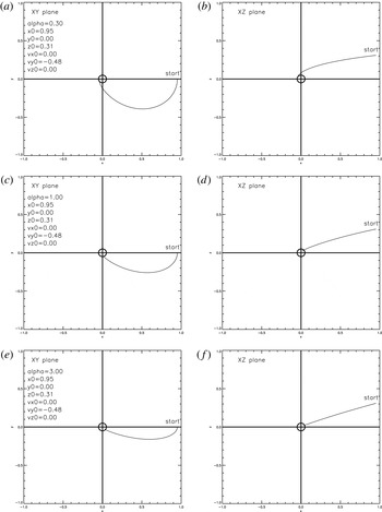
Numerical integration of (8.22a
,
b
) for
 $P_{{\it\phi}}=0$
particle with
 ${\it\alpha}=0.3$
(a,b),
 ${\it\alpha}=1$
(c,d) and
 ${\it\alpha}=3$
(e,f). (a,c,e) Show the projection of the trajectory in the
 $x$
–
 $y$
plane and (b,d,f) show the projection of the trajectory in the
 $x$
–
 $z$
plane. A sphere of radius
 $r=0.05$
with centre at origin is shown to represent a finite-radius source. The particle starts above the
 $z=0$
plane and has a non-chaotic trajectory that impacts the source.

Figure 3 shows trajectories of
 $P_{{\it\phi}}^{\prime }=0$
particles calculated by numerically integrating (8.22a
,
b
) for
 ${\it\alpha}=0.3$
(a,b),
 ${\it\alpha}=1$
(c,d), and
 ${\it\alpha}=3$
(e,f). Figure 3(a,c,e) show the
 $x$
–
 $y$
projection of the trajectory and (b,d,f) show the
 $x$
–
 $z$
projection. The
 ${\it\alpha}=1$
plots (c,d) disprove the generality of the assertion made by Kuzmin & O’Neil (Reference Kuzmin and O’Neil2005) that particle motion is chaotic when
 ${\it\alpha}\approx 1.$
The trajectories in figure 3 show, as predicted, that a
 $P_{{\it\phi}}=0$
particle simply spirals in towards the origin; this is true even if the particle is initially located off of the
 $z=0$
plane. This motion was not considered by Kuzmin & O’Neil (Reference Kuzmin and O’Neil2005) nor by Vrinceanu et al. (Reference Vrinceanu, Granger, Parrott, Sadeghpour, Cederbaum, Mody, Tan and Gabrielse2004) because they did not note that canonical angular momentum is a conserved quantity so the Hamiltonian has the form given by (8.31). Because of this failure to exploit conservation of canonical angular momentum, Kuzmin & O’Neil (Reference Kuzmin and O’Neil2005) and Vrinceanu et al. (Reference Vrinceanu, Granger, Parrott, Sadeghpour, Cederbaum, Mody, Tan and Gabrielse2004) erroneously predicted that for large
 ${\it\alpha}$
(i.e. for
 ${\it\omega}_{c}\gg \bar{{\it\omega}}_{K}$
) particles would always make field-aligned oscillations; the
 ${\it\alpha}=3$
plots (figure 3
e,f) clearly show that a large
 ${\it\alpha}$
particle having
 $P_{{\it\phi}}^{\prime }=0$
does not make a field-aligned oscillation. If different initial values are used, but
 $P_{{\it\phi}}^{\prime }=0$
is maintained, the particles have more complicated trajectories but still eventually fall into the source because there is a force attracting the particles to the source but no repulsive force.
9. Summary
The initial conditions, the electric and magnetic field strengths and the particle sign play various roles. Whether a particle is axis-encircling or not depends only on the sign of
 $P_{{\it\phi}}/(qB)$
and not on the sign or magnitude of the electric field. Only particles with
 $P_{{\it\phi}}=0$
can access the origin. Whether a particle is confined or not depends only on the magnitude of
 ${\it\omega}_{E}^{2}/{\it\omega}_{c}^{2}$
and not on the value of
 $P_{{\it\phi}}$
. Failure to be confined results when there is an excessively steep hill-type potential and this ‘falling off the hill’ corresponds to breakdown of the GCA, to the Brillouin limit and, when there are many adjacent potential hills and valleys, to stochastic trajectories. If the situation is generalized to 3-D and the potential is attractive,
 $P_{{\it\phi}}=0$
particles spiral into the spherical source (e.g. star or classical atomic nucleus).
Acknowledgements
This material is based upon work supported by the U.S. Department of Energy Office of Science, Office of Fusion Energy Sciences under Award numbers DE-FG02-04ER54755 and DE-SC0010471, by the National Science Foundation under Award number 1059519, and by the Air Force Office of Scientific Research under Award number FA9550-11-1-0184.