2.1. Model specification

Lee & Carter (Reference Lee1992) specified the bilinear form:

for the force of mortality on the log scale. The specification (1) differs structurally from parametric models given that the dependence on age is non-parametric, and represented by the sequences of α _x ’s and β _x ’s. Interpretation of the parameters is quite simple: α _x is the general shape of the log-mortality schedule and the actual forces of mortality change according to an overall mortality index κ _t modulated by an age response β _x . The parameter β _x represents the age-specific patterns of mortality change. It indicates the sensitivity of the logarithm of the force of mortality at age x to variations in the time index κ _t . The specification (1) implies that the modelled death rates are perfectly correlated across ages, which is the strength but also the weakness of the approach. As pointed by Lee (2000), the rates of decline at different ages are given by β _x (κ _t −κ _t−1) so that they always maintain the same ratio to one another over time.

The decomposition (1) appears to be very appealing for morbidity rates as well as for various quantities appearing in health insurance, such as age-specific expected claim frequencies or severities. The estimated α _x ’s exhibit the typical shape of the quantity under study (directly or on the log scale). Generally, we get relatively high values around birth, a decrease at infant ages, the accident hump, and finally the increase at adult ages with an ultimately concave behaviour for quantities in line with mortality pattern. Besides the average structure captured by the α _x , the κ _t accounts for time trends that may be due to improvements in longevity, medical inflation, etc. The general time effect κ _t is adapted to each particular age by means of the factor β _x .

In section 3 we explain how to apply (1) to model health insurance expenses.

2.2. Identifiability

In (1), the α _x parameters can only be identified up to an additive constant, the β _x parameters can only be identified up to a multiplicative constant, and the κ _t parameters can only be identified up to a linear transformation. Precisely, if we replace β _x with cβ _x and κ _t with ${{\kappa _{t} } \over c}$ for any c≠0 or if we replace α _x with α _x −cβ _x and κ _t with κ _t +c for any c, we obtain the same values for the death rates. This means that we cannot distinguish between the two parametrisations. A pair of additional constraints are required on the parameters for estimation to circumvent this problem. To some extent, the choice of the constraints is a subjective one, although some choices are more natural than others. In the literature, the parameters in (1) are usually subject to the constraints:

ensuring model identification. Under this normalisation, β _x is the proportion of change in the overall experience attributable to age x (on the log scale).

The lack of identifiability of (1) is only a minor issue. It just means that the likelihood associated with the model has an infinite number of equivalent maxima, each of which would produce identical forecasts. Adopting the constraints (2) consists in picking one of these equivalent maxima. The important point is that the choice of constraints has no impact on the quality of the fit or on forecasts.

2.3. Estimation

Regression models treating age and calendar time as factors are generally used to extract the α _x , β _x and κ _t from the available statistics. The products β _x κ _t make them nonlinear so that standard GLM packages cannot be used. Different distributional assumptions have been proposed so far, including least squares (Lee & Carter, Reference Lee1992), Poisson (Brouhns et al., 2002 Reference Brouhns, Denuit and Vermunta , 2002 Reference Christiansen, Denuit and Lazarb ), Binomial (Cossette et al., Reference Delwarde, Denuit and Partrat2007) and Negative Binomial (Delwarde et al., Reference Denuit, Dhaene, Hanbali, Lucas and Trufin2007) loss functions. The maximum likelihood estimates are easily found using iterative algorithms, that appear to converge very rapidly. The gnm package of the statistical software R (Turner & Firth, Reference Turner and Firth2007) can be used to fit generalised nonlinear models with a score of the form (1), avoiding to develop such algorithms case by case. The numerical illustrations proposed in this paper are performed with gnm.

The specifications listed above remain relevant for morbidity rates or claim frequencies in health insurance, as these quantities are still based on event counts. However, for average severities, discrete distributions are less appealing and the actuary could consider Normal, Gamma or Inverse Gaussian specification, instead.

2.4. Forecast

An important aspect of the decomposition (1) is that the time factor κ _t is intrinsically viewed as a stochastic process. Box–Jenkins techniques are then used to estimate and forecast the time factor within an autoregressive integrated moving average (ARIMA) time series model. These forecasts in turn yield projected age-specific mortality or morbidity rates, as well as severities, on which the calculation of premiums and reserve can be based.

3.1. Data description

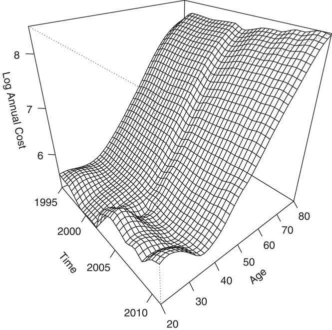
The data set used was issued by the German BaFin. It covers the period 1995−2011. Henceforth, the response Y _x (t) is indexed by attained age x and calendar time t. It describes the average yearly medical inpatient cost for year t=1995, … , 2011 at age x=20, 21, … , 80. The observed y _x (t) are displayed in Figure 1. The shape of the data is similar to a mortality surface, with the increase at young adult ages paralleling the accident hump followed by a linear increase after age 40 similar to the Gompertz part of the mortality schedule, before an ultimate concave behaviour at oldest ages. Surprisingly, the accident hump temporarily vanishes in the calendar years 1999–2001. The effect of medical inflation is also clearly visible, causing an increase in yearly health expenses as time passes.

Figure 1

Observed inpatient costs y _x (t) for German males, t=1995, … , 2011, x=20, 21, … , 80, log scale. Source: BaFin.

The procedure adopted by BaFin for creating the data tables can be summarised as follows. BaFin requires data from all companies, each year, according to different tariffs and types of benefits. The collected data are crude. For each specific table (e.g. inpatient, double room), BaFin smooths the collected crude data with Whittaker-Henderson (with possibly different smoothing parameters for different age groups). There is no further adjustment of the data (except the smoothing).

In this paper, we only consider data for German males. Data for women have been excluded for the following reason. Due to the 2004 European directive on “Equal Treatment in Goods and Services”, 2004/113/EC, pregnancy costs were excluded starting in the BaFin data report in 2007, inducing a break in the data. Our analysis therefore only focusses on male data.

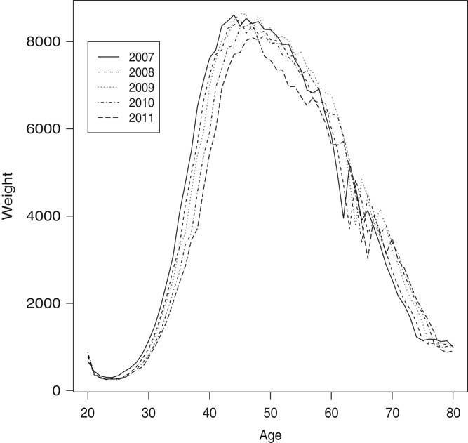
Figure 2 displays the number of policies according to policyholder’s age for each calendar year 2007–2011. This information was missing for years up to 2006. Apart from a moderate ageing effect, the available age-specific numbers appear to be relatively stable over time. Therefore, unavailable volumes for specific years were inferred from observed volumes. Specifically, the age structure has been supposed to be constant over 1995−2006, as suggested by available data.

Figure 2

Number of policies according to policyholder’s age for each calendar year 2007–2011. Source: BaFin.

3.2. The Rusam method

Let us briefly explain how the expected E[Y _x (t)] are modelled on the German market. In German private health insurance, the average yearly claim costs are usually decomposed into

i.e. the expected amount at age x at time t is split into a product of an expected amount at some reference age x ₀ modulated by the age pattern γ _x (t). The profile (or age profile) of the annual medical cost data is thus defined by

for a fixed reference age x ₀, usually x ₀=40.

German private health insurance companies assume that γ _x (t) is approximately constant for at least a short period of time, i.e. γ _x (t)=γ _x (t ₀) for all t in a small interval around t ₀. By defining $\beta _{x}^{{t_{0} }} \,\colon\,{\equals}\, \gamma _{x} (t_{0} )$ and $\kappa _{t}^{{x_{0} }} \,\colon\, {\equals}\, E\left[ {Y_{{x_{0} }} (t)} \right]$ , we obtain the model

The future expected annual medical costs $\kappa _{t}^{{x_{0} }} $ at reference age x ₀ are estimated by linear regression, based on the assumption that

for some real number θ.

The assumption of time constant profiles and perfectly linear time trends are commonly referred to as Rusam method on the German market. However, Figure 1 shows an erratic trend pattern and changes in the profiles with respect to calendar time. Therefore, more sophisticated approaches are needed. In the present paper we try a bilinear approach together with ARIMA time series modelling.

3.3. Modelling approach

In this paper, we relax the linear trend assumption (4) underlying the Rusam approach, and we replace (3) with the specifications

and

involving the bilinear score (1) commonly used in mortality studies with an identity or a log link function, respectively. Similar to Lee & Carter (Reference Lee1992), the decomposition into an age-specific pattern α _x and a time pattern κ _t (trend) modulated by an age response β _x is easy to interpret.

While $$\beta _{x}^{{t_{0} }} $$ and $$\kappa _{x}^{{t_{0} }} $$ in (4) refer to a specific age x ₀ and a specific year t ₀, the variables β _x and κ _t in (5) and (6) are not bound to that restriction. This fact looks negligible, but it is indeed significant when it comes to estimation. Instead of focussing on a specific age and year, the unspecific definition of β _x and κ _t in (5) and (6) reflects the aim to match the data over the full time and age span.

We estimate age profiles α _x and β _x in combination with a time profile κ _t based on all past data. The κ _t are then projected with an appropriate time series model. In contrast to the deterministic trend model (4), the time series approach for κ _t better captures empirically observed patterns and moreover allows to quantify the forecasting uncertainty.

In our case study we consider four different models. All models share similarity with the log-bilinear structure (1) underlying the approach of Lee & Carter (Reference Lee1992). However, we assume continuous distributions for the response variable because we do not have to deal with event counts but average claim severities instead. The models are from the class of generalised non-linear models in the sense that:

• ∙ The response is generated from a distribution of the exponential dispersion family.

• ∙ We specify a link function (logarithm or identity function).

• ∙ The score is not a linear function of the unknown parameters.

3.4. Model comparisons

Henceforth, we consider the following specifications to estimate the parameters α _x , β _x and κ _t appearing in (5) and (6).

M0: Setting α _x equal to 0, the first model is in line with the Rusam method (3) with Y _x (t) Normally distributed with mean β _x κ _t and constant variance σ ², i.e.

For this model, we only normalise the β _x , i.e. we impose the second constraint of (2). Different from the Rusam method, here β _x and κ _t do not refer to a specific year or age. Moreover, for κ _t we allow departures from the linear trend (4).

M1: This model is based on (5) with Y _x (t) Normally distributed, i.e.

This model is close to model M0 except that the set of α _x captures an average level over the observation period.

M2: This model is based on (6) with Y _x (t) Gamma distributed with mean exp(α _x +β _x κ _t ), i.e.

This model differs from M1 to M2 by the distribution assumption (Gamma versus Normal or LogNormal) as well as by the link function (log link versus identity link).

M3: The last model is based on (6) with Y _x (t) Inverse Gaussian, i.e.

This model thus differs from M3 by a different distributional assumption for the response variable (Inverse Gaussian versus Gamma) but not by the link function (log link in both cases).

The models M2 and M3 both use a log link function, which is common in mortality modelling. Different from mortality modelling, we are not modelling claim counts here but claim amounts.

3.5. Model selection

We split the available data set into a training set (calendar years 1995–2008) and a validation set (calendar years 2009–2011). The optimal model is selected on the basis of the accuracy in prediction of the response for the final 3-year period of the data set, in line with the actuarial applications we have in mind.

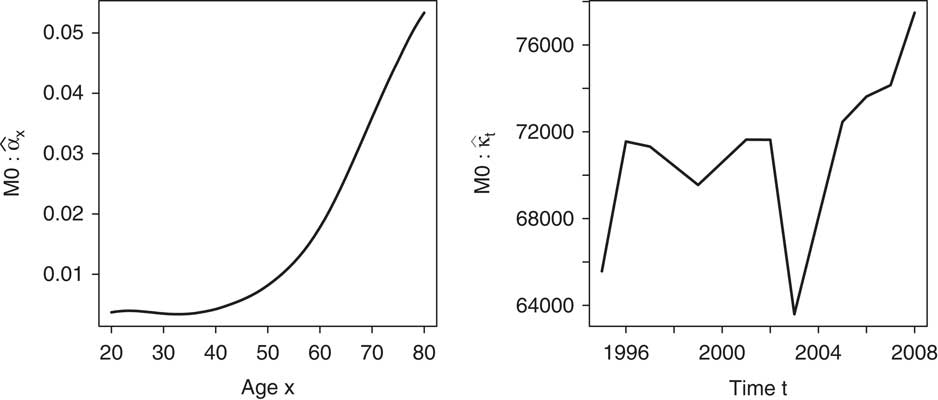
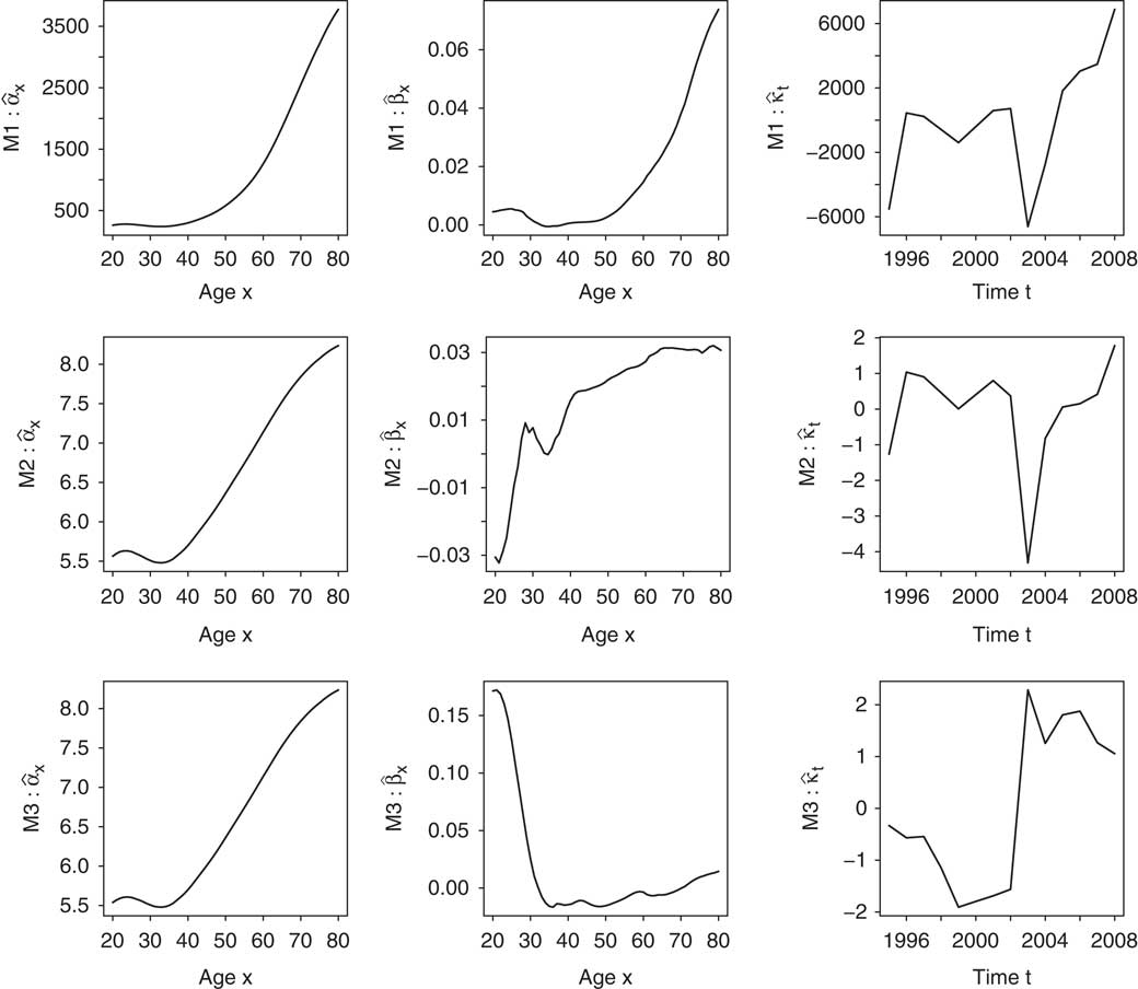
Figures 3 and 4 display the estimated effects for each model M0–M3. Apart from model M2, the estimated effects have a similar pattern across ages or time. Notice the estimated change of sign for β _x in model M2, from negative at younger ages to positive at older ages. As the estimated time index κ _t is increasing, this means that average health costs tend to decrease over time at younger ages, whereas they increase, as expected, at older ages. This is in contrast to the other models, which suggest increasing average health costs at all ages. Considering models M0–M1 on the one hand and model M3 on the other, the shape of the estimated time-sensitivities β _x appears to be reversed. For all models, the data relating to calendar year 2003 looks peculiar, as indicated by the outlying value of $\widehat{\kappa }_{{2003}} $ . This causes a marked break in the series of the estimated time indices.

Figure 3

Estimated effects for model M0.

Figure 4

Estimated effects for models M1–M3.

Since we work in a regression framework, it is essential to inspect the residuals. Model performance is assessed in terms of the randomness of the residuals. Here, we use Pearson residuals for all models M0–M3, computed from $$r_{{xt}} \, {\equals}\, y_{{xt}} {\minus}\widehat{y}_{{xt}} $$ suitably standardised. If the residuals r _xt exhibit some regular pattern, this means that the model is not able to describe all of the phenomena appropriately. In practice, looking at $\left( {x,\,t} \right) \mapsto r_{{xt}} $ , and discovering no structure in those graphs ensures that the time trends have been correctly captured by the model.

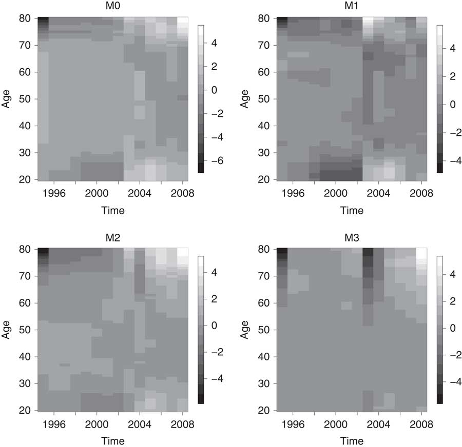
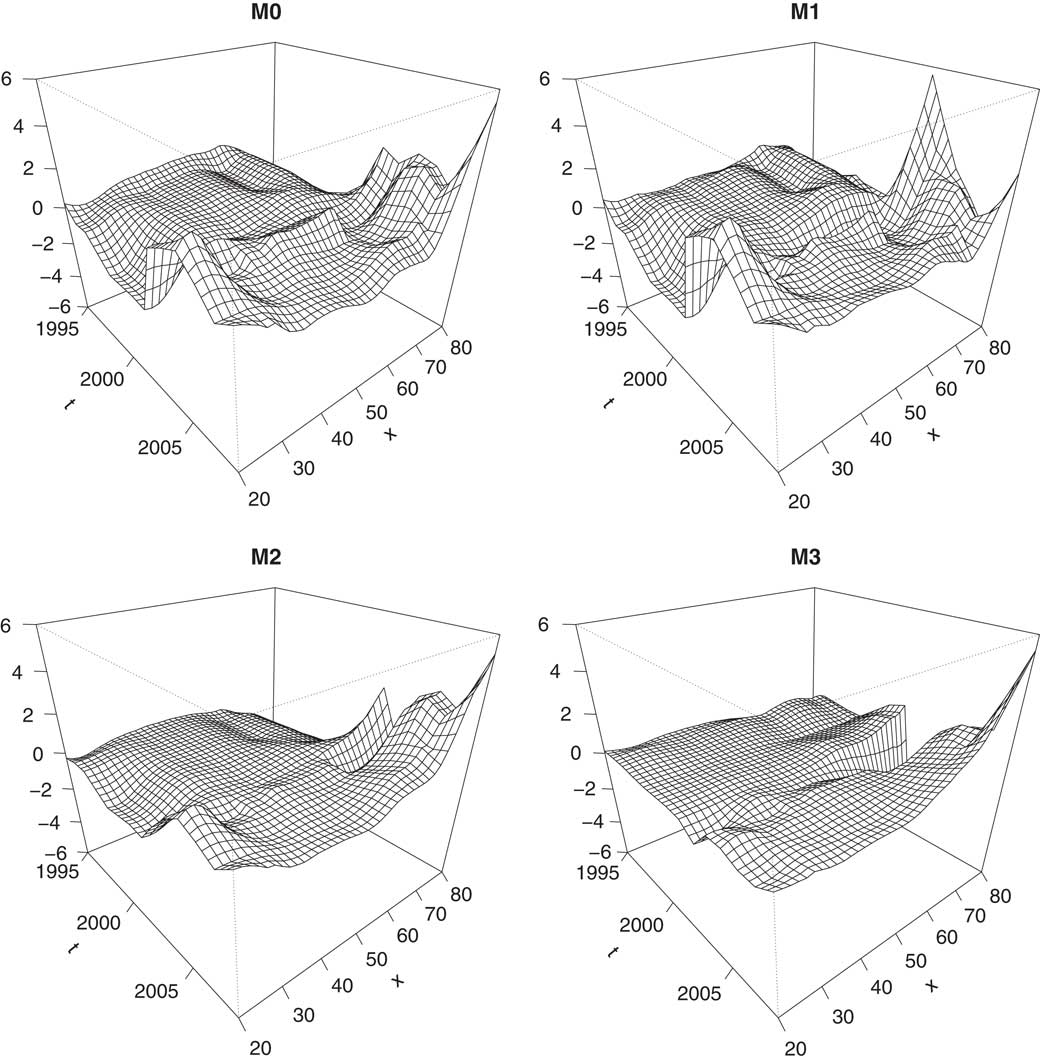
Figures 5 and 6 display the residuals obtained for models M0–M3 as a function of both age and calendar time. Residuals are first inspected with the help of maps in Figure 5. The structure in the residuals can be attributed to the preliminary smoothing procedure implemented by BaFin. This induces similar values for neighbouring cells. This is especially the case for M0. Residuals sometimes assume large positive or negative values near data boundaries but remain generally in the interval [−2, 2]. This is confirmed on Figure 6.

Figure 5

Image plots for standardised residuals r _xt corresponding to models M0–M3.

Figure 6

Standardised residuals r _xt for models M0–M3.

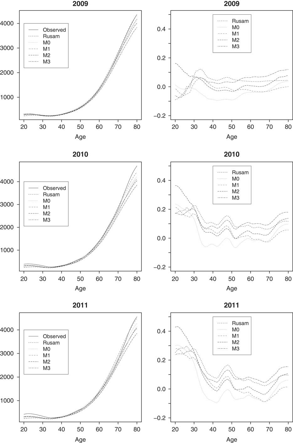
In order to select the best model, we now compare the projections obtained for the last three calendar years 2009–2011 serving as validation set. To this end, the estimated κ _t ’s are viewed as a realisation of a time series that is modelled using the classical ARIMA models. Such models explain the dynamics of a time series by its history and by contemporaneous and past shocks. In line with the standard Lee–Carter approach, estimated κ _t s are projected using an ARIMA (0, 1, 0) time series model. The results are visible on Figure 7. We can see there that the relative differences obtained with M1 outperform the four other models, staying in the range ±5% for 2009 and achieving relative errors <10% for 2010 and 2011, except at younger ages. The Rusam method performs particularly weak in the age range 20–30. In that age range, Figure 1 shows a time pattern that is highly non-linear and clearly different from the time pattern at reference age x ₀=40. Both effects are contrary to the assumptions underlying Rusam’s method. At higher ages, the time pattern becomes more linear and uniform and the difference between methods M0–M3 and Rusam’s method is less profound.

Figure 7

Comparisons of actual y _xt versus predictions obtained from the training set for models M0–M3 with relative differences ${{\left( {y_{{xt}} {\minus}\widehat{y}_{{xt}} } \right)} \mathord{\left/ {\vphantom {{\left( {y_{{xt}} {\minus}\widehat{y}_{{xt}} } \right)} {y_{{xt}} }}} \right. \kern-\nulldelimiterspace} {y_{{xt}} }}$ .

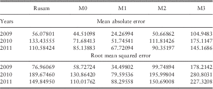
The quality of the prediction is measured with the square root of the mean squared error as well as with the mean absolute error (MAE). Here, the mean squared error is obtained from averaging the squared difference between the observations y _xt for t∈{2009, 2010, 2011} and their prediction $\widehat{y}_{{xt}} $ obtained from the α _x and β _x estimated on the training set combined with the κ _t projected to t≥2009 with the help of the random walk with drift model fitted to the time index of the training period. The MAE is obtained similarly, by taking the absolute differences between observed y _xt for t∈{2009, 2010, 2011} and their prediction $\widehat{y}_{{xt}} $ . The results are reported in Table 1. Based on the performances on the validation set, model M1 appears to be the best one. Note that the weak performance of Rusam’s method at young ages has a rather small impact here since the claim costs are very small at young ages.

Table 1

Root mean squared error and mean absolute error for the validation set.

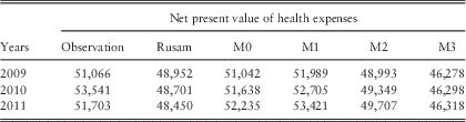
This observation is confirmed by an economic analysis of the prediction results. The net present value of the health expenditure for high ages (starting at age 61) of the observations ∑ _x>60 y _xt ⋅ 1.01^−(x−60) is compared with the value of their prediction $\mathop{\sum}\nolimits_{x\,\gt\,60} {\widehat{y}_{{xt}} \cdot 1.01^{{{\minus}(x{\minus}60)}} } $ for t∈{2009, 2010, 2011}. The yearly discount rate is set to 1%. The results are shown in Table 2. The results reveal that the predictions of Rusam’s method and models M2 and M3 clearly underestimate the health expenses. The weak performance of Rusam’s method at young ages is here dampened by the small weight that young ages have on the total costs. If we focussed on young ages only, the mismatch would increase significantly. Again, the model M1 tends to be the best choice. In particular, the net present value of the prediction only slightly overestimates the net present value of the observations. This is advantageous for risk management purposes.

Table 2

Net present value of health expenses for the validation set.

3.6. Projection

Let us now project the average yearly health claims three years beyond the end of the observation period, thus for calendar years 2012–2014, with the help of the optimal model M1 that has been selected based on the validation set.

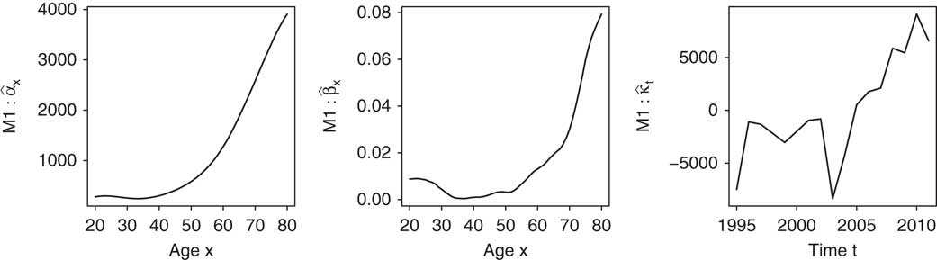
To this end, we first fit this model to the entire observation period 1995–2011. The results are given in Figure 8. The estimated age effect α _x and β _x are similar to those displayed on Figure 4 obtained based on the training set 1995–2008. The time indices are now supplemented with three values, for calendar years 2009–2011 that are now included in the analysis. A linear trend is clearly visible for the $\widehat{\kappa }_{t} $ .

Figure 8

Estimated effects for model M1 fitted to the entire observation period 1995–2011.

Plugging the projected time index to 2014 in the bilinear decomposition provides the actuary with the forecast of health expenditures over the next 3 years. However, this point prediction, while interesting, reveals nothing about the uncertainty attached to the future health costs. In forecasting, it is important to provide information about the error affecting the quantities of interest. In that respect, prediction intervals are particularly useful. In the current application, it is impossible to derive the relevant prediction intervals analytically. The reason for this is that two very different sources of uncertainty have to be combined: sampling errors in the parameters α _x , β _x and κ _t , and forecast errors in the projected κ _t ’s. An additional complication is that the measures of interest E[Y _xt ] are non-linear functions of the parameters α _x , β _x and κ _t , and of the ARIMA parameters. This is why bootstrap procedures are used.

The key idea behind the bootstrap is to resample from the original data (either directly or via a fitted model) in order to create replicate data sets, from which the variability of the quantities of interest can be assessed. Because this approach involves repeating the original data analysis procedure with many replicate sets of data, it is sometimes called a computer-intensive method. Bootstrap techniques are particularly useful when, as in our problem, theoretical calculation with the fitted model is too complex.

If we ignore the other sources of errors, then the confidence bounds on future κ _t ’s can be used to calculate prediction intervals. For mortality studies, we know from Lee & Carter (Reference Lee1992, appendix B), that prediction intervals based on κ _t alone are a reasonable approximation only for forecast horizons of 10–25 years. For long-run forecasts, the error in forecasting the time index thus dominates the errors in fitting the mortality rates. If there is a particular interest in forecasting over the shorter term, as it is the case here, then we cannot make a precise analysis of the forecast errors and prediction intervals based on κ _t alone seriously understate the errors in forecasting over shorter horizons.

This is why we derive here bootstrap percentiles confidence intervals. The bootstrap procedure yields B samples of α _x , β _x and κ _t parameters, denoted as $\alpha _{x}^{b} $ , $\beta _{x}^{b} $ and $\kappa _{t}^{b} $ , b=1, 2, … , B. This procedure can be carried out in several ways (Brouhns et al., 2002 Reference Brouhns, Denuit and Vermunta , 2002 Reference Christiansen, Denuit and Lazarb , Reference Brouhns, Denuit and Vermunt2005; Koissi et al., Reference Koissi, Shapiro and Hognas2006): by Monte Carlo simulation from the approximate multivariate Normal distribution of the maximum likelihood estimators $\widehat{\alpha }_{x} $ , $\widehat{\beta }_{x} $ , and $\widehat{\kappa }_{t} $ , by parametric bootstrap resampling from the fitted model and then re-estimating the age and time effects, or by bootstrapping the residuals.

As reported by Renshaw & Haberman (Reference Renshaw and Haberman2008), the result of Monte Carlo simulation invoking the large sample properties of the maximum likelihood estimators heavily rely on the identifiability constraints. Given that the choice of constraints is not unique and that this choice materially affects the resulting simulations, this first approach should not be used for risk assessment purposes unless there are compelling reasons for selecting a particular set of identifiability constraints. As the preliminary smoothing implemented by BaFin generates local similarities, we conduct parametric bootstrap by generating $y_{{xt}}^{b} $ as realisations from random variables obeying the ${\cal N}or\,\left( {\alpha _{x} {\plus}\beta _{x} \kappa _{t} ,\,\sigma ^{2} } \right)$ distribution. The age and time effects are then re-estimated using the $y_{{xt}}^{b} $ as data points, producing $\alpha _{x}^{b} $ , $\beta _{x}^{b} $ , and $\kappa _{t}^{b} $ , b=1, 2, … , B.

We then estimate the time series model using the $\kappa _{t}^{b} $ as data points. This yields a new set of estimated ARIMA parameters. We can then generate a projection $\kappa _{t}^{b} $ for t beyond the observation period using these ARIMA parameters. In the random walk with drift model, it is enough to add to the last available $\widehat{\kappa }_{t}^{b} $ as many times the drift estimated from the $\kappa _{t}^{b} $ data points as needed to reach the projection horizon.

The first step is meant to take into account the uncertainty in the parameters α _x ’s, β _x ’s and κ _t ’s. The second step deals with the fact that the uncertainty in the ARIMA parameters depends on the uncertainty in the α _x ’s, β _x ’s and κ _t ’s parameters. The third step ensures that the uncertainty of the forecasted κ _t ’s depends on the uncertainty of the ARIMA parameters themselves.

This yields B realisations $\alpha _{x}^{b} $ , $\beta _{x}^{b} $ , $\kappa _{t}^{b} $ and projected $\kappa _{t}^{b} $ on the basis of which we can compute the measure of interest $\widehat{y}_{{xt}}^{b} $ corresponding to E[Y _xt ]. Assume that B bootstrap estimates $\widehat{y}_{{xt}}^{b} $ , b=1, 2, … , B, have been computed. The (1−2α) percentile interval for E[Y _xt ] is given by $\big( {\widehat{y}_{{xt}}^{{b(\alpha )}} ,\,\widehat{y}_{{xt}}^{{b(1{\minus}\alpha )}} } \big)$ , where $\widehat{y}_{{xt}}^{{b(\zeta )}} $ is the 100×ζth empirical percentile of the bootstrapped values for $\widehat{y}_{{xt}}^{b} $ , which is equal to the (B×ζ)th value in the ordered list of replications $\widehat{y}_{{xt}}^{b} $ , b=1, 2, … , B. For instance, in the case of B=1,000 bootstrap samples, the 0.95th and the 0.05th empirical percentiles are, respectively, the 950th and 50th numbers in the increasing ordered list of 1,000 replications of E[Y _xt ].

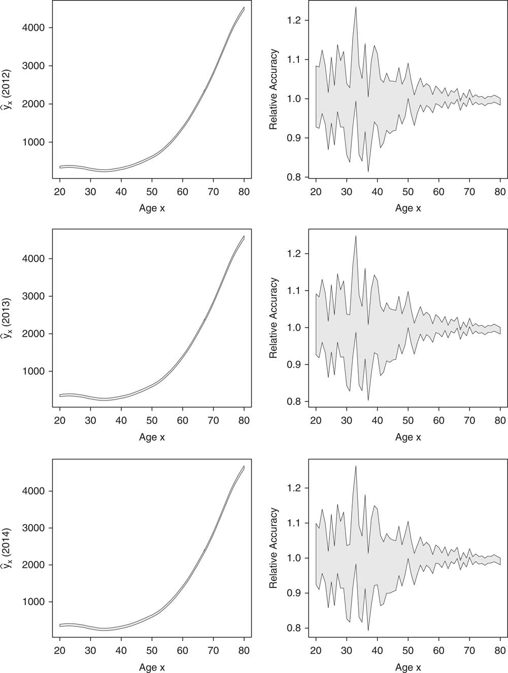
The predictions of E[Y _xt ] for calendar years 2012–2014 are displayed in Figure 9, together with 90% prediction intervals and relative accuracies at the same confidence level (appearing coloured in grey) obtained by parametric bootstrap (with B=1,000). We can see there that the relative accuracy on the expected health insurance claims is generally in the range ±10% at most ages.

Figure 9

Predictions of y _xt with model M1 fitted to the entire observation period 1995–2011 for calendar years 2012–2014 with 90% bootstrap prediction intervals, and corresponding relative accuracies.

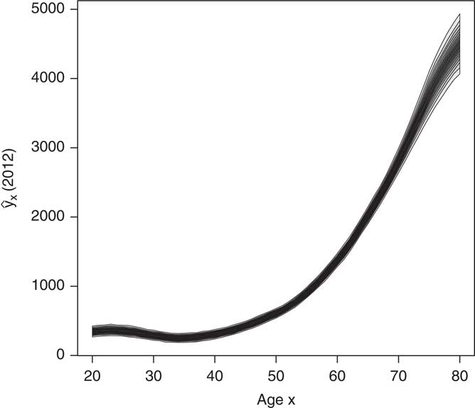
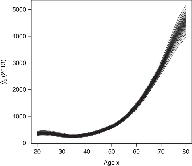
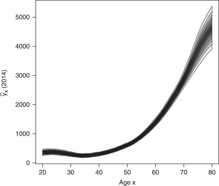
In order to figure out the predictive distribution of Y _xt , we produce analogs to the longevity fan charts proposed by Dowd et al. (2010) based on parametric bootstrap (with B=1,000). The result is shown in Figures 10–12. These charts depict some central projection of the forecasted variable Y _xt , together with bounds around this showing the probabilities that the variable will lie within specified ranges. The difference with the results displayed in Figure 9 if that the time index is now projected to 2012–2014 allowing for some departures from the average trajectory, and that realisations of future Y _xt are finally simulated from the Gaussian distribution. The chart in Figures 10–12 shows the central 10% prediction interval with the heaviest shading surrounded by the 20%, 30%, … , 90% prediction intervals with progressively lighter shading. The shading becomes stronger as the prediction interval narrows. We can therefore interpret the degree of shading as reflecting the likelihood of the outcome: the darker is the shading, the more likely is the outcome. The fan in Figures 10–12 consists of nine grey bands of varying intensity. The upper and lower boundaries correspond to paths of the forecast 95% and 5% quantiles, and the inner edges of the bands in the fan correspond to the 10%, 15%, … , 90% quantiles. The darkest band in the middle is bounded by the 45% and 55% quantiles. Note that the quantiles are calculated for each year in isolation. The fan charts in Figures 10–12 show that short-term departures from the central trend remain limited, except at older ages where the spread is more pronounced.

Figure 10

Fan chart for Y _x (2012).

Figure 11

Fan chart for Y _x (2013).

Figure 12

Fan chart for Y _x (2014).

To end with, let us make a last remark. Future E[Y _xt ] have been obtained using extrapolated κ _t ’s and fixed α _x ’s and β _x ’s. In this case, the jump-off values (i.e. E[Y _xt ] in the last year of the fitting period or jump-off year) are fitted rates. The Lee–Carter method has been criticised by Bell (Reference Brouhns, Denuit and Van Keilegom1997) for the fact that a discontinuity is possible between the observed mortality rates and life expectancies for the jump-off year and the forecast values for the first year of the forecast period. The bias arising from this discontinuity would then persist throughout the forecast. The same comments apply to our setting, and the forecast could start with the last observed y _xt or their average over the end of the observation period.