Introduction
Adaptive optics (AO) retinal imaging tools have substantial potential for use in the diagnosis of retinal degenerations. The improvement in retinal image contrast and resolution allows the direct observation of the cone and rod photoreceptors (Dubra et al., Reference Dubra, Sulai, Norris, Cooper, Dubis, Williams and Carroll2011; Cooper et al., Reference Cooper, Dubis, Pavaskar, Rha, Dubra and Carroll2011; Rossi et al., Reference Rossi, Chung, Dubra, Hunter, Merigan and Williams2011), allowing the opportunity to directly assess pathology early in the disease course. Central to the clinical application of this technology is the ability to quantitatively analyze the photoreceptor mosaic. At present, the majority of studies have focused on the analysis of cone density and spacing of cones (Li & Roorda, Reference Li and Roorda2007; Chui et al., Reference Chui, Song and Burns2008; Li et al., Reference Li, Tiruveedhula and Roorda2010; Dees et al., Reference Dees, Dubra and Baraas2011; Song et al., Reference Song, Chui, Zhong, Elsner and Burns2011; Garrioch et al., Reference Garrioch, Langlo, Dubis, Cooper, Dubra and Carroll2012; Chiu et al., Reference Chiu, Lokhnygina, Dubis, Dubra, Carroll, Izatt and Farsiu2013; Park et al., Reference Park, Chung, Greenstein, Tsang and Chang2013; Ratnam et al., Reference Ratnam, Västinsalo, Roorda, Sankila and Duncan2013; Lombardo et al., Reference Lombardo, Lombardo, Schiano Lomoriello, Ducoli, Stirpe and Serrao2013a ). These studies demonstrate moderate to high variability within cone density and spacing within the healthy adult population, making it difficult to detect small deviations from normal. However, despite individual differences in cone density and spacing, the parafoveal cone mosaic uniformly presents as a triangular lattice, and it is thought that the quality of the cone lattice is of high importance for the interreceptoral network and cell signaling (Hirsch & Miller, Reference Hirsch and Miller1987; Pum et al., Reference Pum, Ahnelt and Grasl1990; Lombardo et al., Reference Lombardo, Serrao, Ducoli and Lombardo2013b ). Thus, disorder in cone packing could serve as an important and sensitive measure with which to characterize a given image of the cone mosaic (Baraas et al., Reference Baraas, Carroll, Gunther, Chung, Williams, Foster and Neitz2007; Wojtas et al., Reference Wojtas, Wu, Ahnelt, Bones and Millane2008).
The geometry of the overall cone mosaic can be easily visualized by defining the Voronoi domain associated with each cone photoreceptor cell in the mosaic. In a perfectly triangular lattice, all cones will have hexagonal Voronoi domains. While numerous investigators have demonstrated that the majority of cones in the normal parafoveal cone mosaic have hexagonal Voronoi domains (Baraas et al., Reference Baraas, Carroll, Gunther, Chung, Williams, Foster and Neitz2007; Li & Roorda, Reference Li and Roorda2007; Carroll et al., Reference Carroll, Rossi, Porter, Neitz, Roorda, Williams and Neitz2010; Wagner-Schuman et al., Reference Wagner-Schuman, Neitz, Rha, Williams, Neitz and Carroll2010; Dees et al., Reference Dees, Dubra and Baraas2011; Dubra et al., Reference Dubra, Sulai, Norris, Cooper, Dubis, Williams and Carroll2011; Lombardo et al., Reference Lombardo, Serrao, Ducoli and Lombardo2013b ; Lombardo et al., Reference Lombardo, Serrao, Ducoli and Lombardo2013c ), there are only a few examples of using mosaic geometry to detect retinal pathology in AO imagery. Baraas et al. (Reference Baraas, Carroll, Gunther, Chung, Williams, Foster and Neitz2007) imaged individuals with congenital tritan color vision deficiency and observed density within normal limits but significantly disrupted regularity, with the percentage of six-sided Voronoi cells being substantially lower (55%) than normal controls (70%). The authors concluded that the short-wavelength sensitive (S-) cones degenerated in these patients, with the observed normal density explained by the fact that the S-cones comprise only about 5% of the total number of cones (which is significantly smaller than the known inter-individual variability in cone density).
Further insight into the packing regularity of the cone mosaic comes from assessment of the orientation of individual cones within the mosaic. Previous work has shown that the human cone mosaic forms a variable number of hexagonal submosaics that differ in orientation and are separated by cones with nonhexagonal arrangements (Pum et al., Reference Pum, Ahnelt and Grasl1990; Ahnelt & Kolb, Reference Ahnelt and Kolb2000). Algorithms for assessing the orientation of the cone mosaic were originally developed for use in histological images, but to our knowledge have not been applied to AO images of the cone mosaic. Thus, the aim of the present work was to demonstrate two new methods for analyzing the anisotropy and orientation of cones in simulated and real AO images of the parafoveal cone mosaic. These methods were based on Fourier (Meitav & Ribak, Reference Meitav and Ribak2011) and Radon transforms (Deans, Reference Deans1983) and were compared to a previously developed algorithm (Pum et al., Reference Pum, Ahnelt and Grasl1990). We demonstrate that the orientation of individual cones within the mosaic can be accurately measured using these techniques.
Materials and methods
Three algorithms were implemented to assess the orientation of a set of photoreceptors in images using MATLAB (Mathworks Inc, Natick, MA). Each algorithm was tested on both simulated and real images of the cone photoreceptor mosaic. For each image, cone photoreceptor coordinates were used to derive a Voronoi diagram for the mosaic. The number of neighbors of a given cone was defined as the number of sides of the Voronoi polygon corresponding to that cone’s location. Only orientation information for cones with six neighbors was obtained with each algorithm.
Neighbor derived orientation
Spatial orientation analyses assay local neighborhoods of individual cones. For a given cone location, nearby neighbors can be identified either by distance (Pum et al., Reference Pum, Ahnelt and Grasl1990) or by using a Voronoi diagram (Curcio & Sloan, Reference Curcio and Sloan1992). The original method in Pum et al. (Reference Pum, Ahnelt and Grasl1990) selected the seven nearest neighbors, and excluded any cones outside ±30% of the median neighbor distance. Cells within the ±30% median distance “band” were used for analysis. Curcio and Sloan (Reference Curcio and Sloan1992) modified this step to use the neighbors defined by the Voronoi diagram of the cone centers. Both methods limited further analysis to those cones with only six neighbors.
In the neighbor-derived orientation, a vector is created from the central cone to each neighbor. Pum et al. (Reference Pum, Ahnelt and Grasl1990) used the median-distance neighbor to define an initial reference vector, and computed the difference between that vector and the vector from the central cone to each of the other neighbors, adjusting the differences in angle to lie between ±30°. These adjusted vectors plus the original reference vector were added and divided by 6 to yield a “characteristic vector” which contained information about size and orientation of a hexagon centered on that central cone (Pum et al., Reference Pum, Ahnelt and Grasl1990). Curcio and Sloan (Reference Curcio and Sloan1992) used a slightly different method of computing orientation, which took the median of the adjusted vectors and reference vector to create the “characteristic vector,” though this yielded similar results to the method of Pum et al. (Reference Pum, Ahnelt and Grasl1990). Both produce a characteristic orientation which ranges over 60° because of the presumed six-way symmetry of the hexagonal neighborhood. Due to concerns regarding the reliability of the median-based characteristic vector, the Pum algorithm was used throughout this manuscript.
Fourier derived orientation
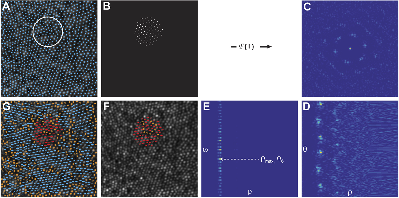
Fourier spectral analysis is intrinsically insensitive to cones missed or misidentified in the image and provides global, reliable information on their spacing, arrangement, and periodicity. Based on this premise, a spectrum angular Fourier method was performed on several overlapping circular regions of interest (ROIs) (e.g., two adjacent areas were 50% overlapped), I(x,y), with a diameter 4.5 times greater than the inter-cell distance (ICD) of the given mosaic (Fig. 1). The ROI size was chosen empirically to balance stability and sensitivity; substantially larger (>6 times the ICD) ROIs caused the algorithm to be insensitive to local variations, whereas substantially smaller (<3 times the ICD) ROIs caused the algorithm to produce highly variable results. The power spectrum of each ROI was derived from the discrete Fourier transform (DFT): f(u,v) = DFT(|I(x,y)|2), and converted to polar coordinates f(ρ,θ). All DFTs were performed using the fast Fourier transform (FFT). In general f(ρ,θ) can be written as a sum of cosine angular function components:
 $$f\left( {\rho ,\theta } \right) = {A_0}\left( {\rho ,\theta } \right) + \sum\limits_{n = 1}^\infty {{A_n}\left( {\rho ,\theta } \right)\,\cos \left[ {n\left( {\theta - {\phi _n}\left( {\rho ,\theta } \right)} \right)} \right]} \quad ,$$
where A n (ρ,θ) and ϕ n (ρ,θ) are the amplitude and the phase of the nth Fourier harmonic components of f(ρ,θ), respectively. The information on the packing arrangement, such as spacing and orientation, can be retrieved by taking the 1-D Fourier transform on the angular content of the power spectrum of eqn. (1), as follows:
 $$F\left( {\rho ,\omega } \right) = {\rm{FFT}}\left( {{{\left| {f\left( {\rho ,\theta } \right)} \right|}^2}} \right)\quad ,$$
by evaluating the modulo component and the phase of eqn. (2).
Outline of the steps to retrieve the orientation of individual cones using the Fourier method. (A) Individual cones in an AOSLO image of the cone mosaic are identified using a cone identification algorithm, and the mean inter-cell neighbor distance is calculated. A region of interest (ROI; white circle) with a diameter 4.5 times greater than the ICD is sampled uniformly across the image such that each ROI overlaps by 50% with each of its neighboring ROIs. (B) For each ROI, a binary mask is used to generate an image of the cone coordinates, I(x,y). (C) The power spectrum, f(u,v) = DFT(|I(x,y)|2), is calculated for each ROI and converted to polar coordinates, f(ρ,θ), as shown in (D). (E) Next, a 1-D FFT is performed on the angular content of the power spectrum of F(ρ,Θ) = FFT(|f(ρ,ω)|2). The spatial characteristic length scale, associated with the hexagonal arrangement of the cones within the ROI, is defined as d hex = 1/ρ max, in which ρ max represents the maximum value of the module F(ρ,6). (F) The corresponding local mean orientation of the hexagonal arrangement is calculated as ϕ 6 = −arg(F(ρ max,6)/6) and it expresses the average angular hexagonal neighbor orientation for each ROI. (G) The final orientation for each six-sided cell is computed by taking the mean of average angular hexagonal neighbor orientations of the ROI in which that cell fell. Non six-sided cells are shown as open circles in (F) and (G). The AO image subtends a 120 × 120 µm area.

The sixth spectrum component, F(ρ,6), contains frequency information about the six equidistant vertices, regardless of the orientation of the hexagonal packing. For each ρ value, the modulus F(ρ,6) represents the size of the hexagonal arrangement and its corresponding phase represents the local hexagonal packing orientation. If we extract the value ρ max, which represents the maximum value of the module F(ρ,6), the corresponding d hex = 1/ρ max can be identified as the spatial characteristic length scale associated with the hexagonal arrangement on the ROI. The corresponding local mean orientation of the hexagonal arrangement is calculated as ϕ 6 = −arg(F(ρ max,6))/6 and defined as the average angular hexagonal neighbor orientation. The average angular hexagonal neighbor orientation was calculated for each ROI, and the orientation of each cone was determined by averaging the orientations of each ROI that overlapped the cone’s location. The algorithm steps are shown graphically in Fig. 1.
Radon derived orientation
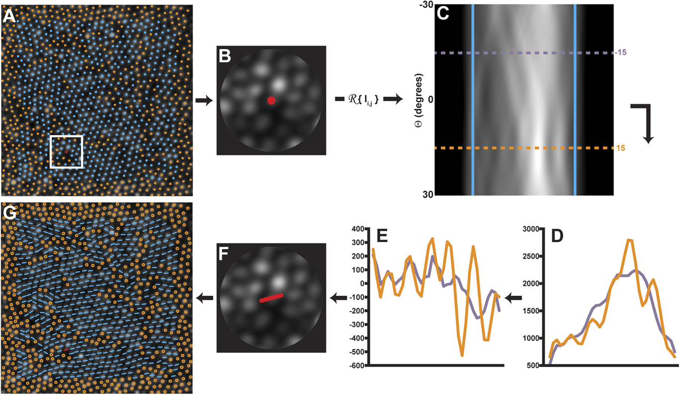
Another approach was derived using the Radon transform (Deans, Reference Deans1983). The Radon transform is an integral transform typically performed over a series of straight “projection” lines. The inverse of the Radon transform is used extensively in reconstruction of medical computed tomography images (Herman & Kuba, Reference Herman and Kuba1999). Here, we used the Radon transform to assess orientation by determining the projection angle, which typically occurs along the orientation of the cones. To accomplish this, a ROI that was 4.5 times the mean ICD was extracted at each cone location (Fig. 2A). This ROI size was empirically determined to be ideal; a larger ROI was insensitive to local changes in orientation, while a smaller ROI was too sensitive to local changes, and had noisy results. A circular mask was applied to each ROI (Fig. 2B), and each ROI was transformed using the Radon transform
 $$f\left( {r,\theta } \right) = R\left( {I{{\left( {x,y} \right)}^2}} \right)\quad ,$$
where θ is the angle of the projection and r is the projection bin. In the Radon-transformed ROI, each row (θ) was an angle and each column was a projection bin (r) (Fig. 2C). Because the rotation of a hexagon can only be detected over a −30 to 30° range, only θ between the values of 60 and 120° (where 90° is horizontal) were considered.
Outline of the steps used to determine the orientation of individual cones using a Radon transform. (A) A ROI 4.5 times the ICD is centered on each cone with a six-sided Voronoi domain is selected within the image. (B) A circular mask is applied to the ROI. (B and C) The Radon transform is applied to the ROI and the sides of the transform are smoothed with a Gaussian filter (fifth order, σ = 0.75) and cropped (blue lines). Each cropped row of (C) contains information from each angle θ of Radon projection. (D) Shows the projection profiles at two rows corresponding to −15° (purple profile) and 15° (orange profile). To determine the row with the most contrast, the second derivative of each row is performed (E), and the row θ with the highest RMS (orange profile) is selected as the orientation at that location. A low RMS location (purple profile) is shown for comparison. (F) The orientation is assigned to that cell. (G) The algorithm is repeated for each six-sided cell location in the image. The adaptive optics image subtends a 120 × 120 µm area.

When a Radon transform is oriented along the axis of the photoreceptors contained in a ROI, it creates a characteristic multi-peak pattern along across the projection bins (r) (Fig. 2D, orange profile) corresponding to the dominant orientation at that location. This information can be extracted from the Radon transform by assessing the row (θ) at which the multiple-peak pattern is most resolvable. To mitigate the effect of image noise on our measurement of the multiple peaks, each row (θ) was smoothed with a Gaussian filter (fifth order, σ = 0.75), and the second order derivative of the smoothed row was calculated. The central region of the row was cropped to exclude the masked area using the first and last zero-crossings, and the root-mean-square (RMS) of the cropped, differentiated profile was calculated along each row. The row with the maximum RMS was taken as the main orientation of the ROI. Footnote 1
Algorithm validation
To assess the accuracy of the algorithms, a simulated cone mosaic with perfect hexagonal packing was created as an idealized model of the human parafoveal cone mosaic. The simulated mosaic subtended 150 × 150 µm with a 0.45 µm/pixel, and the cone spacing (ICD = 3.64 μm) corresponded to a density of 87,000 cones/mm2. The relationship between spacing and density is consistent with that of a perfect hexagonal mosaic, according to methods described by Coletta and Williams (Reference Coletta and Williams1987). The coordinates were rotated (between ±30°; with 1° step), and then cropped to a 120 × 120 µm area for analysis. From this set of coordinates, an accompanying cone “image” was generated by convolving a 2D Gaussian with a binary mask at each of the cone locations. Each algorithm was run on each rotated cone mosaic. The results of each algorithm were then compared to the known rotation (Fig. 3A).
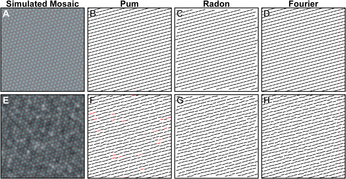
Comparison of orientation algorithms using an 87,000 cones/mm2 simulated mosaic without (A) and with (E) cone intensity variation and coordinate jitter. The neighbor derived orientation (Pum et al., Reference Pum, Ahnelt and Grasl1990) algorithm correctly determines the orientation of the mosaic without any coordinate jitter [(B), black orientation bars], but can produce results outside of tolerance (>|3°|, red orientation bars) when the coordinates are jittered and cone intensity varied (F). Both the Radon (C and G) and Fourier (D and H) algorithms are insensitive to coordinate jitter and image intensity variability.

We further examined the accuracy of the algorithms in the presence of noise by perturbing the coordinates in the perfect mosaics by a random amount drawn from a Gaussian distribution with a mean of 0 and a s.d equivalent to 5% of the cone spacing (0.21 μm, Fig. 3B). Additionally, the intensity of each cone in the image was adjusted by randomly selecting an intensity from a log-normal distribution with a 24.9 A.U. (arbitrary units) s.d. and mean intensity of 80 A.U., based on cone reflectivity values previously observed in AO images from normal subjects (Cooper et al., Reference Cooper, Dubis, Pavaskar, Rha, Dubra and Carroll2011).
Testing algorithm performance
To examine the performance of each algorithm on a more “realistic” simulated mosaic, we generated mosaics that contained multiple submosaics of differing local orientation (Fig. 4). A 130 × 130 µm area (0.45 µm/pixel scale) was created, and 20 locations from within the area were randomly drawn from a uniform distribution and used as seed locations for each submosaic. Each seed location was assigned a random rotation within a range of ±30°, and new cones were added radially to each seed, separated by an azimuth of 60° and a radius defined by an ICD of 3.64 μm so as to maintain a hexagonal lattice affixed at the seed’s assigned orientation. This process was repeated for each cone until encountering another cone. Once no more cones could fill the area, the cone locations were “relaxed” 100 times using a “hard disk” model similar to that proposed by Stillinger et al. (Reference Stillinger, DiMarzio and Kornegay1964) (Supplemental Video 1). The final mosaic was then cropped to a 120 × 120 µm area for analysis. One hundred simulated mosaics, which contained 77 ± 2% six-sided Voronoi cells, were created in this manner. An accompanying cell image was generated for each simulated mosaic as previously stated, and all three algorithms were then run on each simulated image.
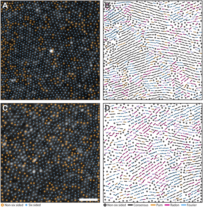
Comparison of orientation algorithms using simulated mosaics. Algorithm agreement in simulated mosaics with a highest (A and B) and lowest (C and D) agreement. Cyan circles mark six-sided cell locations, while orange circles mark unanalyzed, non-six sided cells. Black bars are locations where at least two algorithms agreed within their combined tolerances (6°). Each color in the right column corresponds to results from each algorithm (Pum: orange, Radon: magenta, Fourier: cyan). If one algorithm was outside tolerance, a bar with the corresponding color was overlaid on the black bar. If all three algorithms disagreed, the orientation from each method is plotted. Scale bar is 20 µm.

Finally, each algorithm was tested using 17 images acquired from 17 subjects using a custom adaptive optics scanning light ophthalmoscope (AOSLO) (Dubra & Sulai, Reference Dubra and Sulai2011). This research was conducted according to the tenets of the Declaration of Helsinki, and image acquisition was approved by the institutional research boards at the Medical College of Wisconsin and Marquette University (Milwaukee, WI). AOSLO images were acquired using a 790 nm scanning beam over a 1.0° field of view, 0.5° temporal from fixation was imaged in each subject. Axial length measurements were obtained on all subjects using an IOL Master (Carl Zeiss Meditec, Dublin, CA), and used in combination with a simplified Gullstrand II model to convert from degrees of visual angle to micrometers on the retina. The central 120 × 120 µm was cropped from each image. Cone coordinates were semiautomatically identified using a previously described algorithm (Garrioch et al., Reference Garrioch, Langlo, Dubis, Cooper, Dubra and Carroll2012). The spacing of cones and their packing arrangement were analyzed using ICD and a Voronoi tessellation, which was used to extract the percentage of six-sided cones. The Pum, Fourier, and Radon algorithms were run on each image as described above.
Analysis of algorithm performance
To examine algorithm accuracy in the rotated versions of a “perfect” simulated mosaic, we compared the orientation of each six-neighbor cone to the known rotation of the simulated mosaic (Fig. 5). The detected orientation of each cone from each algorithm was subtracted from the known rotation for evaluating the error. A tolerance interval ±3° of the known rotation was used to account for rounding error and noise. Any cone orientations which fell outside the tolerance interval were considered incorrect.
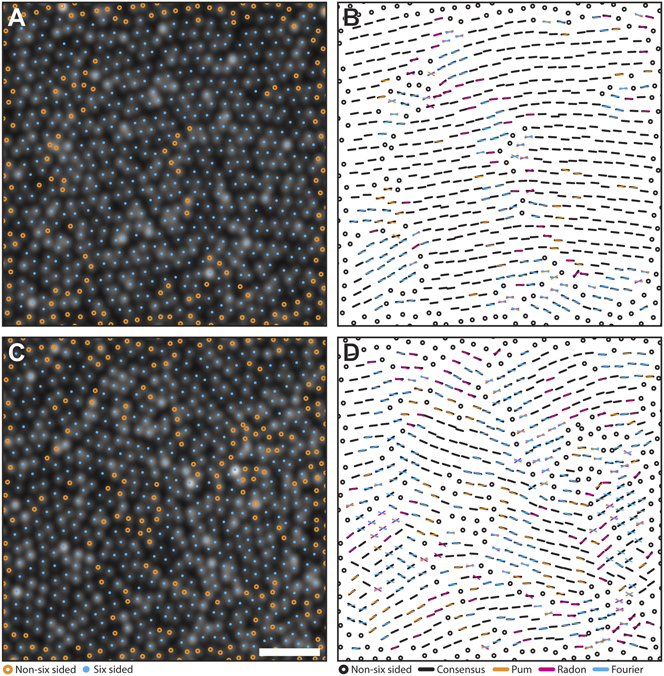
Comparison of orientation algorithms using real mosaics. Algorithm agreement in AOSLO images of the parafoveal cone mosaic with a highest (A and B) and lowest (C and D) agreement. Cyan circles mark six-sided cell locations. Orange circles mark to unanalyzed, non-six sided cells. Black bars are locations where at least two algorithms agreed within their combined tolerances (6°). Each color in the right column corresponds to results from each algorithm (Pum: orange, Radon: magenta, Fourier: cyan). If one algorithm was outside tolerance, a bar with the corresponding color was overlaid on the black bar. If all three algorithms disagreed, the orientation from each method is plotted. Scale bar is 20 µm.

For simulated mosaics containing multiple submosaics or real images of the cone mosaic collected using AOSLO, we compared the algorithms by estimating submosaic homogeneity. Homogeneity was determined by overlaying a grid with 15 × 15 µm spacing on each mosaic. The variance of the orientation of cells within each grid square was calculated. Homogeneity was defined as the average pooled variance across all grid squares. Pooled variance describes the average spread of all grid variances about their mean; the higher the pooled variance in this analysis, the lower the submosaic homogeneity by a given algorithm.
We measured algorithm agreement using both the Pearson correlation coefficient and the ICC based on a two-way random model. The Pearson correlation coefficient was calculated to estimate the correlation between algorithm pairs, and the ICC was used to estimate the reliability between orientations from all three algorithms. All statistical analyses were performed in SPSS (IBM, Armonk, NY). Data were expressed as mean ± s.d. (M ± s.d.).
Results
Simulated mosaic performance
For the rotated versions of the ideal simulated mosaic, each algorithm was able to correctly assess the amount of rotation applied to the mosaic. Fig. 3 exemplifies the ability of each algorithm to detect the orientation of a perfectly hexagonal mosaic either in the absence or presence of noise. In a perfect mosaic (Fig. 3A), correct identification of cone orientation within the ±3° tolerance was achieved for 100, 99.8, and 100% of cones using the Pum, Fourier, and Radon approaches, respectively (Fig. 3B–3D). The Fourier algorithm’s 0.2% error was due to the perfect lattice with no rotation; the hexagonally located coordinates created artifacts in the Fourier domain, causing the algorithm to return erroneous values. Given that this only occurred in an extreme (and nonphysiologic) case, we considered the algorithm’s performance to be equivalent to that of the other two. The average absolute errors were 0.06 ± 0.02°, 0.11 ± 0.04°, and 0.10 ± 0.24°, using the Pum, Fourier, and Radon approaches, respectively. When noise in the form of coordinate jitter and cone intensity variation was applied to the image (Fig. 3E), correct identification of cone orientation within the ±3° tolerance was achieved for 95.8, 99.9, and 99.9% of cones using the Pum, Fourier, and Radon approaches, respectively (Fig. 3F–3H). The average absolute errors for the noisy mosaic were 1.18 ± 0.04°, 0.15 ± 0.08°, and 0.22 ± 0.26°, for the Pum, Fourier, and Radon algorithms, respectively. Taken together, these results demonstrate excellent accuracy for all three algorithms.
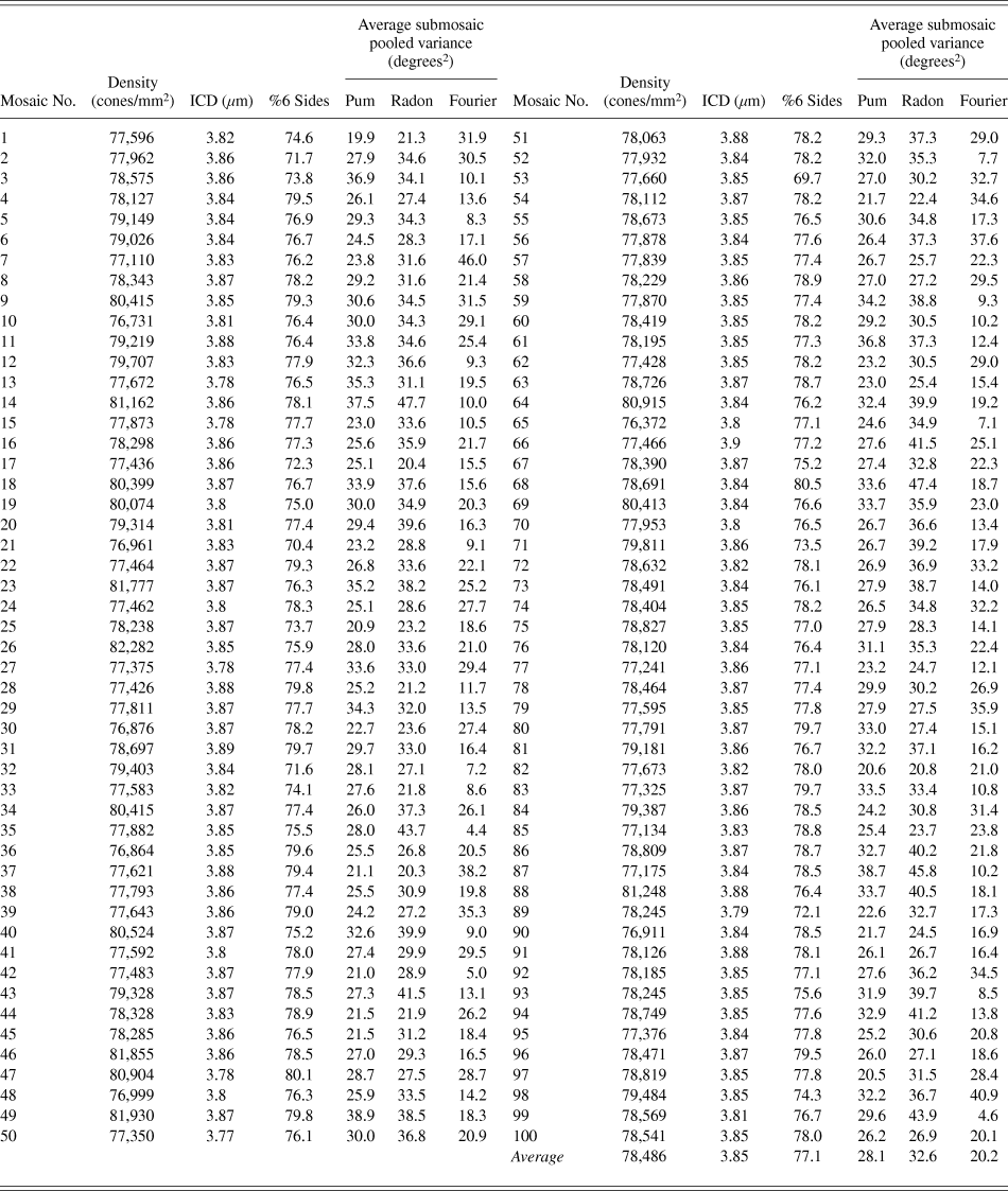
The 100 simulated mosaics containing multiple submosaics had an average of 76.9 ± 2.1% six-sided Voronoi cells, and an average ICD of 3.8 ± 0.03 µm. This ICD was slightly larger (5.5 ± 0.7%) than the ICD derived from the average density of each simulated mosaic (78,486 ± 1262 cones/mm2). This was consistent with previous observations that within the photoreceptor mosaic there are point and line discontinuities, where the hexagonal lattice is disrupted (Pum et al., Reference Pum, Ahnelt and Grasl1990; Ahnelt & Kolb, Reference Ahnelt and Kolb2000). The presence of these disruptions in the mosaic reduces the number of ideally packed cones, increasing the measured ICD. Qualitatively, we found that both the Pum and Fourier methods were particularly susceptible to artifacts around the edges of six-sided submosaics; this was likely related to noise from neighboring nonhexagonal cones. On average, the Fourier method was the most homogenous with a 20.2 ± 9.0 degrees2 pooled variance across all submosaics, while the Pum and Radon methods showed pooled variances of 28.1 ± 4.5 and 32.6 ± 6.3 degrees2, respectively (Fig. 4). The results from each simulated mosaic are summarized in Table 1. We found that the Radon and Pum methods correlated more closely (r = 0.92; P < 0.01) than the Radon and Fourier methods (r = 0.85; P < 0.01) and the Pum and Fourier methods (r = 0.84; P < 0.01). The average ICC for all pairwise correlations among all three algorithms was 0.95.
Simulated mosaic descriptive metrics summary

Real mosaics
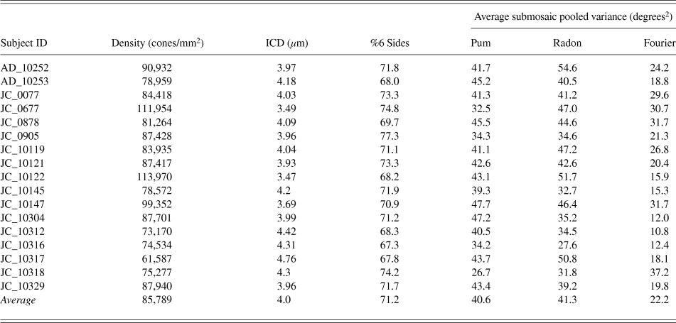
The real photoreceptor mosaics from 17 subjects contained on average 71 ± 3% six-sided Voronoi cells. The average density was 85,789 ± 13,251 cones/mm2, and average ICD was 4.0 ± 0.3 µm. Using each mosaic’s density to calculate the expected ICD for a perfect triangular lattice (Coletta & Williams, Reference Coletta and Williams1987), we again found that the measured ICD was consistently larger (9.0 ± 0.8%) than the ICD derived from the mosaic density. When examining the orientation of the real mosaics, only the Fourier algorithm had an average pooled variance similar to the simulated parafoveal mosaics (22.2 ± 7.9 degrees2, Fig. 5). In contrast, the Pum and Radon methods were less homogenous than the simulated mosaics with average pooled variances of 40.6 ± 5.6 and 41.3 ± 7.9 degrees2, respectively. The decreased homogeneity of both the Pum and Radon methods could be due to the lower percentage of six-sided Voronoi cones in real mosaics; on average, there were 5.9% less hexagonal cones in real mosaics than in simulated mosaics. While the orientation of nonhexagonal cones is not calculated for either algorithm, their presence still influences the orientation of neighboring hexagonal cones, potentially decreasing the observed homogeneity. Despite the decreased homogeneity in real mosaics, we found that the Radon and Pum methods still correlated more closely (r = 0.87; P < 0.01) than the Radon and Fourier methods (r = 0.82; P < 0.01) and the Pum and Fourier methods (r = 0.82; P < 0.01). The average ICC for all pairwise correlations among all three algorithms was 0.94. The results from each AOSLO dataset are summarized in Table 2.
AOSLO descriptive metrics summary

Discussion
In this work, we have shown the performance of a previous orientation detection algorithm (Pum et al., Reference Pum, Ahnelt and Grasl1990), as well as two new approaches to detecting cone orientation. The algorithms had very good reliability across both simulated (0.95) and real mosaics (0.94), suggesting that each algorithm would provide an accurate description of photoreceptor orientations when applied to the coordinates (Pum and Fourier) or directly to an image (Radon). Analysis of inter-algorithm correlations highlighted the differences between the Fourier method and the Pum and Radon methods; we found a lower correlation between the Fourier and Pum algorithms and the Fourier and Radon algorithms than between the Pum and Radon algorithms. This is likely due to orientation averaging present in the Fourier algorithm. Specifically, the orientation of a cell of interest determined by the Fourier algorithm is the average of that cell’s orientation and the orientations of its surrounding cells. This is in contrast to the Pum and Radon methods, which do not average surrounding orientations. The intrinsic “regional averaging” performed in the Fourier method allows the algorithm to be robust to single-cell changes in orientation, and this property was reflected by submosaic homogeneity that was consistently lower than the other two algorithms in both artificially generated and real data (Tables 1 and 2), but similar between the Pum and Radon algorithms. However, regionally averaging multiple orientations can result in inaccuracies near the edges of submosaic patches where non six-sided cells and submosaics with different dominant orientations meet (Pum et al., Reference Pum, Ahnelt and Grasl1990; Curcio & Sloan, Reference Curcio and Sloan1992; Lombardo et al., 2013Reference Lombardo, Serrao, Ducoli and Lombardo b ; Lombardo et al., Reference Lombardo, Serrao, Ducoli and Lombardo2013c). Understanding this difference as well as other algorithm limitations is essential to understand the specific utility of each algorithm. For example, the reliability of the Fourier and Pum approaches is directly linked to the accuracy of the cone identification algorithms that provide their coordinates. Cone identification algorithms can miss cones, identify extra cones, or incorrectly identify a cone’s centroid (Lombardo et al., Reference Lombardo, Serrao and Lombardo2014); each of these scenarios could affect the results of Pum approach; since the Fourier approach provides an average orientation of the cones in a ROI, it is less sensitive to this error. Likewise, the Fourier method is able to overcome cell coordinate imprecision, or “jitter,” because any small differences in coordinate location are integrated when the coordinates are first transformed (Fig. 1D), whereas the Pum method can return an erroneous result if the axis of the jitter is perpendicular to the circumference of the polygon formed by neighboring cones. This limitation can be seen in the ideal mosaic results (Fig. 3), where the accuracy of the Pum method decreases markedly from 100 to 95.8% in the presence of coordinate jitter.
In contrast to coordinate-centric approaches, the Radon method is performed directly on the image, and only uses the cone coordinates to determine which locations to analyze. Because the algorithm is performed directly on the image, the algorithm requires image quality sufficient enough to resolve inter-cell spacing. Therefore, any image with poor cell resolution due to either poor image quality or an insufficient system resolution will cause the algorithm’s result to be unreliable. Moreover, the Radon algorithm cannot determine the orientation of cells near the edge of an image without using some form of correction (edge replication, mirroring, or padding). A benefit of image-based methods is that they do not require cell coordinates, and in principle, orientation could be determined at each pixel within an image, removing the requirement of predetermined cell coordinates. An image-only approach could also be used in the Fourier algorithm. However, future work is needed to understand the reliability of the Fourier method using only the retinal image.
As each algorithm accurately defines orientation in ideal mosaics, the primary difference between the algorithms is how each responds to input imprecision. This could directly influence which algorithm is applied. For example, the Fourier algorithm appears to be the most robust to poor signal-to-noise ratio and poor cell identification precision. This makes it an ideal candidate for instances where the data reliability is poor. Conversely, in situations where there is high image quality, the Radon algorithm could be preferred to retrieve directly the cones orientation. Finally, in cases where both the image and cell coordinate reliability is excellent, Pum’s method would be expected to perform best.
Cell orientation has the potential to detect subtle changes in photoreceptor regularity, but there are numerous other aspects of orientation that still need to be examined. Principle among them is the effect of eccentricity on orientation. It has been established that the percentage of six-sided cells increases away from the fovea and peaks at approximately 0.5° before decreasing to foveal levels at 1° and beyond (Baraas et al., Reference Baraas, Carroll, Gunther, Chung, Williams, Foster and Neitz2007; Li & Roorda, Reference Li and Roorda2007; Carroll et al., Reference Carroll, Rossi, Porter, Neitz, Roorda, Williams and Neitz2010; Dees et al., Reference Dees, Dubra and Baraas2011; Lombardo et al., Reference Lombardo, Serrao, Ducoli and Lombardo2013b ). The effect of the percentage of six-sided cells, e.g., by analyzing real mosaics collected beyond 1°, was not explored in this manuscript, although we would expect that the orientation of cone photoreceptors would be far less homogenous due to the loss of the hexagonal lattice. Other phenomena that may contribute to the orientation of hexagonal cones as a function of eccentricity are local variance of the cone shape and the compression along the vertical meridian as a consequence of the expansion along the horizontal meridian of the photoreceptor mosaic; the effect of these properties could be explored in a future work.
In addition to the effect of eccentricity on orientation, it has not yet been determined how the orientation of a mosaic changes in response to retinal pathology. Nevertheless, the results from each algorithm suggest that the orientation of individual cones is not random, but correlated to their neighbors, consistent with previous observations (Pum et al., Reference Pum, Ahnelt and Grasl1990; Curcio & Sloan, Reference Curcio and Sloan1992). Thus, deviations in the expected orientation of neighbors within the cone mosaic could be used as a metric of photoreceptor structure, especially when used as a complement to conventional cone metrics such as cell density and spacing. Indeed, the most commonly used mosaic descriptors are not directionally sensitive, and only provide distance measurements derived from cone positions. Measurements of cone regularity, like cell orientation, have the potential to measure a unique aspect of the structure of a photoreceptor mosaic. As the clinical utility of AO devices continues to expand (Carroll et. al., Reference Carroll, Kay, Scoles, Dubra and Lombardo2013), the development of novel, sensitive metrics are essential to characterizing the human photoreceptor mosaic.
Supplementary Data
Supplemental materials can be viewed in this issue of VNS by visiting http://journals.cambridge.org/VNS.
Acknowledgments
The authors would like to acknowledge the contributions of Phyllis Summerfelt for her administrative assistance, and Christopher S. Langlo, Melissa Wilk, Brian Higgins, Erika Phillips, and Moataz Razeen for imaging assistance. Research supported in this publication was supported in part by the National Center for Research Resources and the National Center for Advancing Translational Sciences of the National Institutes of Health under Award No. UL1TR000055 and by the National Eye Institute of the National Institutes of Health under Award Nos. R01EY017607 and P30EY001931. Its contents are solely the responsibility of the authors and do not necessarily represent the official views of the NIH. Funding also provided by the Italian Ministry of Health (5 × 1000 funding; M.L.), Fondazione Roma (M.L.) and the National Framework Program for Research and Innovation PON (Grant No. 01_00110; G.L.).