





1. Introduction
Passive flow control using vane-type miniature vortex generators (MVGs) with heights smaller than 50 % of boundary layer thickness (Lin Reference Lin1999, Reference Lin2002; Shahinfar et al. Reference Shahinfar, Sattarzadeh, Fransson and Talamelli2012) has exhibited promising effects in various scenarios, e.g. the transition delay of laminar boundary layers (Fransson & Talamelli Reference Fransson and Talamelli2012; Shahinfar et al. Reference Shahinfar, Sattarzadeh, Fransson and Talamelli2012), boundary layer separation control (Lin Reference Lin1999; Angele & Muhammad-Klingmann Reference Angele and Muhammad-Klingmann2005; Godard & Stanislas Reference Godard and Stanislas2006; Lögdberg Reference Lögdberg2006), and noise reduction in cavity flows (Che et al. Reference Che, Chu, Schmidt, Cao, Likhachev and Wu2019; Wang et al. Reference Wang, Ye and Shao2025) and supersonic jets (Liu et al. Reference Liu, Khine, Saleem, Lopez Rodriguez and Gutmark2022; Saleem et al. Reference Saleem, Karnam, Rodriguez, Liu and Gutmark2023). Within the context of transition delay in a two-dimensional boundary layer, MVG arrays generate high- and low-speed streaks to modify spanwise velocity, leading to the attenuation of Tollmien–Schlichting (TS) waves and localised disturbances (Fransson & Talamelli Reference Fransson and Talamelli2012; Siconolfi et al. Reference Siconolfi, Camarri and Fransson2015), and can result in a net skin-friction drag reduction up to 65 % (Sattarzadeh et al. Reference Sattarzadeh, Fransson, Talamelli and Fallenius2014). As a passive control tool, MVG arrays are able to generate additional embedded streamwise vortices in laminar boundary layers and advantageously induce streaks through the lift-up mechanism (Fransson & Talamelli Reference Fransson and Talamelli2012; Shahinfar et al. Reference Shahinfar, Sattarzadeh, Fransson and Talamelli2012; Siconolfi et al. Reference Siconolfi, Camarri and Fransson2015). Through direct numerical simulation (DNS) and a local spatial stability analysis, Siconolfi et al. (Reference Siconolfi, Camarri and Fransson2015) found that MVG designs that generate high-amplitude streaks result in a stronger initial amplification of TS waves near the wake region of the MVGs. More recently, Szabó et al. (Reference Szabó, Nagy, De Baets, Vanierschot and Paál2024) optimised MVGs for the stability control of laminar boundary layers. They reported that streak properties in the boundary layer, e.g. the maximum amplitude and streamwise extent, are controllable by manipulating the streamwise vortex properties.
Summary of experimental and numerical studies associated with the characterisation and evolution of vane-type MVG-induced streamwise vortices in canonical TBLs. The quantity
 $\delta$
is the boundary layer thickness,
 $h$
is the MVG height,
 $l$
is the MVG chord length and
 $d$
is the spanwise spacing for a VG pair. Here,
 $\alpha$
is the wing angle of attack relative to the streamwise direction. These geometrical parameters are also seen in figures 1(a) and 1(b). Additionally,
 $ \textit{Re}_{\delta } = U_{\infty }\delta /\nu$
is the Reynolds number based on freestream velocity
 $U_{\infty }$
and
 $\delta$
.

MVGs are also of great interest in the flow separation control of turbulent boundary layers (TBLs) due to their performance in transferring sufficient momentum from the outer region to the near-wall region (e.g. Lin Reference Lin2002). In this regard, fundamental research pertaining to MVGs has focussed on the separation control of adverse pressure gradient boundary layers in low-speed flows (Lin et al. Reference Lin, Howard and Selby1991; Lin Reference Lin1999) and shock waves in supersonic flows (McCormick Reference McCormick1992; Mounts Reference Mounts1992), as well as the characterisation and correlation of MVG-induced streamwise vortices in TBLs. It is found that MVGs with a device height
 $h$
approximately 20 % of boundary layer thickness,
 $\delta$
, are as effective as conventional vortex generators (VGs) (with
 $h$
of the order of
 $\delta$
) in delaying or preventing boundary layer separation with low device drag and without sacrificing efficiency (Lin Reference Lin2002). Many studies since 2000 have focused on the characterisation and evolution of MVG-induced streamwise vortices as well as their interactions with TBLs (Ashill et al. Reference Ashill, Fulker and Hackett2001; Yao et al. Reference Yao, Lin and Allan2002; Lögdberg et al. Reference Lögdberg, Fransson and Alfredsson2009; Chan & Chin Reference Chan and Chin2022b
; Sun et al. Reference Sun, Philip, Schröder and Klewicki2025). Table 1 lists the representative studies associated with the characterisation and the evolution of MVG-induced streamwise vortices in canonical TBLs. In this regard, Ashill et al. (Reference Ashill, Fulker and Hackett2001, Reference Ashill, Fulker and Hackett2002) developed a correlation of vortex strength with device Reynolds numbers (
 $h^+ = u_{\tau }h/\nu$
, where
 $u_{\tau }$
is the friction velocity and
 $\nu$
is the kinematic viscosity of fluids) and examined the influence of spacing between MVGs on the strength of counter-rotating vortices. They found that the spacing has potential benefits in preventing the reduction in vortex strength downstream of MVGs. Detailed flow field data were also obtained by Yao et al. (Reference Yao, Lin and Allan2002) through stereo PIV and two-dimensional Reynolds-averaged Navier–Stokes (RANS) simulations. They found that the magnitude of maximum vorticity increases with increasing angle of attack of MVGs, while the peak vorticity and circulation show an exponential decay rate and are inversely proportional to the distance downstream from the MVG. Lögdberg et al. (Reference Lögdberg, Fransson and Alfredsson2009) experimentally investigated the evolution of synthetic streamwise vortices at moderately high Reynolds numbers. These vortices were generated from geometrically self-similar MVG pairs and arrays with a height
 $h$
between 22 % and 67 % of
 $\delta$
. They found that the vortex core experiences a hook-like motion in the cross-flows farther downstream of the MVGs. The circulation of these vortices is scaled by
 $h$
and the local velocity at the tip of the MVGs. Moreover, the turbulence quantities show strikingly scaling behaviour with
 $h$
in the streamwise direction.
More recently, high-resolution numerical simulations provided details regarding the interactions between the MVG-induced streamwise vortices and existing small- or large-scale flow structures in TBLs. Employing wall-resolved LES, Chan & Chin (Reference Chan and Chin2022a
) investigated the characteristics of a moderate-Reynolds-number canonical TBL perturbed by an MVG array with
 $h/\delta = 0.19$
. They found that the relatively large-scale streamwise vortices significantly transported high-momentum fluid from the outer to near-wall region, inducing alternating high- and low-speed streaks that persist up to 500
 $h$
downstream of the MVG. Under proper selection of geometrical parameters, these vortices and induced streaks are capable of dramatically reorganising the coherent structures in TBLs. In a subsequent work, they numerically investigated the influence of MVG arrays on the Reynolds shear stress distributions using a triple velocity and scale decomposition (Chan & Chin Reference Chan and Chin2022b
). These detailed numerical and experimental studies have significantly deepened the understanding of the dynamics concerning the evolution of embedded streamwise vortices, and their interactions with the small- and large-scale motions in naturally occurring TBLs. While informative, these studies mainly focus on the modifications of TBLs due to synthetic streamwise vortices of relatively large scale (i.e. larger
 $h/\delta$
). There also remains limited understanding of the dynamical distinctions that regulate the evolution of these larger-scale streamwise vortices.
The evolution of small-scale embedded streamwise vortices in low-friction-Reynolds-number TBLs has been recently investigated by the present researchers (Sun et al. Reference Sun, Philip, Schröder and Klewicki2025) using wall-resolved LES. It was found that small-scale streamwise vortices, generated from a pair of near-wall vortex generators (NWVG) with a height of
 ${\sim}30$
wall units, have a spanwise scale similar to that naturally occurs in TBLs. These small-scale vortices (and streaks) also exhibit a strikingly similar signature of kinetic energy transport with their natural near-wall counterparts. It was further found that these synthetic vortices are wholly resident to the near-wall region. This is an apparent distinction from the dynamical signature pertaining to the evolution of the larger-scale vortices studied by Lögdberg et al. (Reference Lögdberg, Fransson and Alfredsson2009) or Chan & Chin (Reference Chan and Chin2022a
). The large-scale vortices generated in both of these studies are capable of continuously developing to influence the outer region and even the entire boundary layer. An important question here, therefore, is whether there is an underlying physical mechanism that can characterise the dynamics associated with the evolution of introduced streamwise vortices of different sizes and that then can be used to distinguish their wall-normal domain of influence.
Boundary layers with embedded streamwise vortices are three-dimensional wall-bounded turbulent flows subject to secondary flow effects (Bradshaw Reference Bradshaw1987). Generally, synthetic streamwise vortices in a TBL endure over a finite time scale. Thus, the influence of these introduced vortices inevitably vanishes from TBLs. It is known, however, that for a given Reynolds number, the wall-normal development of naturally occurring TBLs is also finite as expressed by
 $\delta$
. Whether the wall-normal influence of finite liftetime synthetic streamwise vortices encompasses the entire TBL over an
 $\mathcal{O}(\delta )$
streamwise development is, however, an open question. To investigate this question, we examine the evolution of MVG-sourced streamwise vortices of different sizes, with an emphasis on their wall-normal influence. From the viewpoint of understanding boundary layer dynamics, this also offers insights pertaining to the selection of a perturbation to influence the large-scale motions in the background turbulence.
The present work complements previous studies regarding the characterisation and evolution of MVG-induced streamwise vortices in canonical TBls through planar PIV measurements and wall-resolved LES data, from the perspective of momentum transport signatures and the mean momentum balance. The focus is to investigate the scale effect of the evolution of the introduced streamwise vortices in low-friction-Reynolds-number TBLs. These counter-rotating streamwise vortices, ranging from small to relatively large spanwise scales, are generated by a family of geometrically self-similar vane-type MVGs of different heights smaller than 50 % of boundary layer thickness. Specifically, a primary aim is to identify the physical mechanisms that describe the evolution of small, ‘mesoscale’ and relatively large streamwise vortices with respect to their wall-normal domain of influence and the momentum transport signatures. A second objective is to characterise a scale that determines whether a synthetic vortex pair will evolve to ‘escape’ from the near-wall region.
The remainder of this paper proceeds as follows. Section 2 describes numerical and experimental details. This includes numerical methods, experimental set-up and cases investigated. The geometrical parameters of MVGs are also described. Section 3 examines the instantaneous flow field of TBLs perturbed by small-scale and mesoscale synthetic vortices. Section 4 presents the main results of flow statistics concerning TBLs with or without synthetic vortices. Then,
 $\S$
5 describes the definition of the escape scale of synthetic vortices and its estimate based on the analyses in
 $\S$
§ 4.1–4.4. Section 6 presents conclusions.
2. Numerical and experimental details
Section 2.1 first gives the range of LES and PIV measurement cases investigated to show how these datasets are designed to be complementary. Section 2.2 then describes numerical details, including the numerical method and computational set-up. In
 $\S$
2.3, the experimental section describes the facilities, the PIV configuration and the set-up used to generate synthetic varying-size streamwise vortices that are generated from a family of geometrically self-similar MVGs.
2.1. Cases investigated
All synthetic vortices in the present simulations and experiments were generated via geometrically similar MVGs. Readers are referred to §§ 2.2 and 2.3 for more information about the geometry of the VGs. Overall, three groups of rectangular MVGs were used to generate varying-size synthetic vortices: (i) near-wall vortex generators (NWVGs); (ii) mesoscale vortex generators (MEVGs); and (iii) relatively large vortex generators (LVGs). Here, all the VGs have a height smaller than
 $0.5\delta$
. Although the VGs can flexibly generate synthetic vortices in experiments, the spanwise evolution of the vortices is difficult to accurately capture and measure. The previous considerations thus motivate us to use wall-resolved LES in combination with planar PIV measurements (in the streamwise and wall-normal plane) to quantify these flows.
Table 2 lists the LES and PIV measurement cases. TBLs containing embedded synthetic streamwise vortices are labelled with the type of MVGs, while those without synthetic vortices are labelled as a zero-pressure-gradient (ZPG) case. The boundary layer Reynolds numbers cited in table 2 correspond to the position where the MVGs are placed in cases S2, S4, S5 and E2–E4. As we shall see in §
 $\S$
3–5, VG cases E2–E4 and S4–S5 are those mainly used for analyses.
Numerical and experimental cases of TBLs containing geometrically similar MVGs in S2, S4, S5, E2–E4. The name of LES and PIV measurement cases is denoted by SX and EX (e.g. S1 and E1), respectively. The Reynolds number information is for the boundary layer at a streamwise position where the MVGs are placed in TBLs. NWVGs, MEVGs and LVGs are used to generate synthetic streamwise vortices of small, meso- and large scales, respectively.

The smooth-wall TBL (S1, S3 and E1) was first simulated and experimentally measured. This allowed determination of the inner length scale (where
 $u_{\tau }$
is the friction velocity and
 $\nu$
is the kinematic viscosity). Table 2 documents the MVG properties. In particular, small synthetic vortices are generated by the NWVGs with heights
 $h^+ = hu_{\tau }/\nu$
= 24 and 30, while relatively larger ones are produced by MEVGs or LVGs having
 $h^+$
= 48 or 96. Here, it is useful to note that the circulation of TBL synthetic vortices is scaled with
 $h$
and the streamwise velocity at the VG tip,
 $U_{h}$
(Angele & Muhammad-Klingmann Reference Angele and Muhammad-Klingmann2005; Lögdberg et al. Reference Lögdberg, Fransson and Alfredsson2009). Furthermore, the study of Lögdberg et al. (Reference Lögdberg, Fransson and Alfredsson2009) suggests the spanwise scale of the synthetic vortices is approximated by
 $h$
for near-field positions downstream. To simplify the following descriptions, the terms ‘small’, ‘mesoscale’ and ‘large’ are used to describe the synthetic vortices generated from the MVGs of
 $h^+ = 24$
(or 30 for case S2), 48 and 96, respectively. The maximum
 $\delta ^+$
for smooth wall experiments is approximately 270 due to the flow speed limit of the water tunnel. LES cases (S3, S4 and S5) at a lower
 $ \textit{Re}_{\tau }$
(
 ${\sim}235$
) are thus performed to match experiment parameters and minimise
 $\delta ^+$
effects from comparisons. Sections 2.2 and 2.3 provide more details regarding the wall-resolved LES and PIV measurements.
2.2. Numerical details
2.2.1. Numerical method
A high-resolution monotone integrated large-eddy simulation (MILES) (Boris et al. Reference Boris, Grinstein, Oran and Kolbe1992) was used to simulate the flows with and without MVGs. The MILES method implicitly models the effect of the unresolved smallest scales through numerical dissipation. The compressible continuity, momentum and energy equations can be described by the non-dimensional arbitrary Lagrangian–Eulerian formulation,
 \begin{align} \frac {\text{d}}{\text{d}t} \int _{V(t)} \boldsymbol{Q} \,\text{d}V + \oint _{A(t)} \boldsymbol{(\underline {H}^{\textit{in}v} - \underline {H}^{v\textit{is}})}\boldsymbol{\cdot }\boldsymbol{n} \,\text{d}A = 0, \end{align}
with the vector of conservative variables
 $ \boldsymbol{Q} = [\rho , \rho u, \rho v, \rho w, \rho E]^T$
. Here,
 $A(t)$
is the surface of the time-varying control volume
 $V(t)$
. The inviscid and viscous flux tensors,
 $\boldsymbol{\underline {H}}^{\textit{in}v}$
and
 $\boldsymbol{\underline {H}}^{v\textit{is}}$
, are given by
 \begin{align} \boldsymbol{\underline {H}^{\textit{in}v} - \underline {H}^{v\textit{is}}} = \begin{bmatrix} \rho (\boldsymbol{u} - \boldsymbol{u}_A) \\[3pt] \rho \boldsymbol{u} (\boldsymbol{u} - \boldsymbol{u}_A) + p \boldsymbol{\underline I} \\[3pt] \rho E (\boldsymbol{u} - \boldsymbol{u}_A) + p \boldsymbol{u} \end{bmatrix} - \frac {1}{Re_0} \begin{bmatrix} 0 \\[3pt] \boldsymbol{\underline \tau } \\[3pt] \boldsymbol{\underline \tau } \boldsymbol{u} - \boldsymbol{q} \end{bmatrix}\!. \end{align}
Here, the density is
 $\rho$
and the velocity vector is
 $\boldsymbol{u}$
. The velocity of the control volume surface is
 $\boldsymbol{u}_A$
and the pressure is
 $p$
. Here,
 $\rho$
,
 $\boldsymbol{u}$
,
 $p$
are the primitive variables. The total energy is
 $E = e + ({1}/{2}) \boldsymbol{u^2}$
and the unit tensor is
 $\boldsymbol{\underline I}$
. Neglecting bulk viscosity, the stress tensor
 $\boldsymbol{\underline \tau }$
is given by
 \begin{align} \boldsymbol{\underline \tau } = \mu (\boldsymbol{\nabla u} + \boldsymbol{\nabla u}^T) - \frac {2}{3} \mu (\boldsymbol{\nabla \boldsymbol{\cdot }u}) \boldsymbol{\underline I}, \end{align}
and the conductive heat flux is
 \begin{align} \boldsymbol{q} = -\frac {\mu }{Pr_0(\gamma - 1)} \boldsymbol{\nabla } T, \end{align}
where Sutherland’s law is used to compute the dimensionless dynamic viscosity
 $\mu = T^{1.5} ({1+S})/({T+S})$
and
 $S$
is the Sutherland constant that is set to
 $S = {111}/{293}$
. The Reynolds number
 $ \textit{Re}_0 = \rho _0^{\ast } a_0^{\ast } L^{\ast }/\mu _0^{\ast }$
is based on the sound speed at the stagnation state with
 $a_0^{\ast } = \sqrt {{\gamma p_0^{\ast }}/{\rho _0^{\ast }}}$
. Here, the specific heat ratio
 $\gamma = c_{p,0}^{\ast }/ {c_{V,0}^{\ast }}$
is 1.4 and the characteristic length
 $L^\ast$
is 1 m. The dimensionless vector of heat conduction,
 $\boldsymbol{q}$
, is evaluated at a constant Prandtl number
 $Pr_0 = 0.72$
. The governing equation is complemented by the ideal gas equation in dimensionless form,
 $p = {\rho T}/{\gamma }$
. The speed of sound
 $a$
for the ideal gas satisfies
 $a = \sqrt {\gamma p/\rho } = \sqrt {T}$
. In the previous descriptions, the superscript
 $(\ast )$
denotes dimensional variables, i.e. the reference values at the stagnation state. Note that the Mach number
 $ \textit{Ma}$
is 0.1 for the present simulations to approximate the incompressible boundary layer flow. The dimensionless freestream values of the primitive variables are given by
 $T_{\infty } = 1/(1 + 0.5(\gamma -1) Ma^2)$
,
 $U_{\infty } = Ma\sqrt {T_\infty }$
and
 $p_\infty = \gamma ^{-1} T_\infty ^{\gamma /(\gamma -1)}$
.
The governing equations are discretised by a cell-centred finite-volume method (FVM) on locally refined Cartesian grids with cut cells at the boundaries (Schneiders et al. Reference Schneiders, Günther, Meinke and Schröder2016). Spatial discretisation of the viscous flux
 $\underline {H}^{v\textit{is}}$
is performed by central difference with second-order accuracy. The inviscid flux
 $\underline {H}^{\textit{in}v}$
is discretised by a mixed central-upwind advective upstream splitting method (Liou & Steffen Reference Liou and Steffen1993; Meinke et al. Reference Meinke, Schröder, Krause and Rister2002). Time integration is performed using a 5-stage Runge–Kutta scheme, which leads to second-order accuracy in time.
2.2.2. Computational set-up
The ZPG TBL simulation cases are S1 and S3, and the perturbed TBLs are cases S2, S4 and S5. Cases S1 (ZPG TBL) and S2 (with NWVGs) are taken as examples to show the simulation set-up. A wall-resolved LES of a ZPG TBL (case S1) was performed first to design the NWVG case. A schematic of the computational domain for case S2 is shown in figure 1(
 $a$
). Here,
 $x$
,
 $y$
and
 $z$
denote the streamwise, wall-normal and spanwise directions, respectively. The dimensions of the computational domain are
 $l_x = 22\delta _0$
,
 $l_y = 10\delta _0$
and
 $l_z = 2.8\delta _0$
, corresponding to streamwise, wall-normal and spanwise distances. Here,
 $\delta _0$
is the inflow boundary layer thickness. As shown in table 3, the smallest grid cell size at the wall is 0.92 wall units, while the largest (at the upper edge of the boundary layer) is 7.36 wall units. The total cell number
 $N_{\textit{cell}}$
in case S1 is approximately 4.42
 $\times$
 $10^8$
. In case S2, locally refined cells are employed around the NWVGs, where the grid cells near the NWVGs have the same resolution as at the wall (see table 3). The total cell number in case S2 is approximately 4.76
 $\times 10^8$
.
Details of numerical set-up for the LES of a ZPG TBL (case S1, S3) and TBL containing embedded NWVGs (case S2, S4), MEVGs (case S5). The NWVG pair is located at
 $ \textit{Re}_\tau$
= 440, which is the friction Reynolds number of the ZPG TBL at the corresponding positions. Similarly, NWVGs in case S4 and MEVGs in case S5 are located at
 $ \textit{Re}_\tau$
= 235. The inner properties to scale the height of the vortex generators are also from the ZPG TBL at the same location.

The NWVG pair in case S2 is placed at a streamwise position of approximately 15
 $\delta _0$
from the inlet. The friction Reynolds number is
 $ \textit{Re}_\tau =$
440 and the momentum thickness Reynolds number is
 $ \textit{Re}_\theta =$
1322. Streamwise positions are measured relative to the trailing edge of the NWVGs. As shown in figure 1(
 $b$
), the height of the NWVG is
 $h^+ = 30$
 $(h = 0.08\delta _0)$
with a length
 $l$
of
 $3h$
and width
 $w$
of
 $0.33h$
. The spacing
 $d$
at the trailing edge of the NWVG pair is
 $2.53h$
 $(d^+ = 75.9)$
. The wing angle of the NWVG pair is fixed at
 $15^\circ$
relative to the streamwise direction. Note that the NWVGs (cases S2 and S4) and MEVGs (case S5) are geometrically similar, as mentioned in
 $\S$
2.1. The geometrical parameters (
 $\alpha$
,
 $l$
and
 $d$
) follow the VG design of Lögdberg et al. (Reference Lögdberg, Fransson and Alfredsson2009). This design criterion was initially proposed by Pearcey (Reference Pearcey1961) for the design of conventional VGs to ensure that the synthetic vortices have a vortex strength effective to persist in the streamwise direction. Simulation details in cases S3–S5 are similar to those in S1 and S2. The main differences are shown in table 3.
Sketch of (
 $a$
) the computational domain, (
 $b$
) the geometrical parameters of the NWVG pair and (
 $c$
) the synthetic turbulence generation (STG) at the inlet of the domain.

To reduce computational cost, synthetic turbulence is generated near the inlet and reorganised along the plate, as shown in figure 1(
 $c$
). This flow evolves into a canonical TBL at a streamwise position that is roughly 10 initial boundary layer thickness downstream of the inlet. Readers are referred to Roidl et al. (Reference Roidl, Meinke and Schroeder2013) for more details on this synthetic turbulence generation method. Characteristic outflow conditions are applied at the downstream boundary of the domain. A symmetry condition is applied at the upper boundary of the domain. Periodic conditions are applied in the spanwise direction.
2.3. Experimental set-up
2.3.1. Flow facility
The experiments were conducted in the recirculating water tunnel in the Wet Lab at the University of Melbourne. The test section of this facility has a dimension of 1140
 $\times$
460
 $\times$
460 mm. For all experiment cases, the pump rotation speed was set to 1600 rpm to avoid inducing excessive vibrations that influence the measured turbulent fluctuations. The water level is fixed at 460 mm. The freestream velocity
 $U_{\infty }$
was 0.228 ms
 $^{-1}$
for all cases. The water was regularly filtered to minimise the potential influence of impurities on the PIV measurements.
Sketch of the experimental set-up of planar PIV measurements in the
 $y{-}x$
plane. (
 $a$
) Side view. (
 $b$
) Top view. There are four measured streamwise windows (
 $W_1$
,
 $W_2$
,
 $W_3$
and
 $W_4$
) at the downstream position of MVGs. Two spanwise positions are selected for measurement, i.e.
 $z = 0$
(central plane of the MVG pair) and
 $z_1 = 1.5h$
.
 $h$
is the height of the corresponding MVG. The measurement range in the
 $x$
direction is approximately 10
 $\delta$
.
 $\delta$
is the boundary layer thickness (in the smooth-wall TBL) measured in the first field of view (i.e.
 $W_1$
) that is near the trailing edge of the MVG pair.

2.3.2. Planar PIV measurement and data reduction
Figure 2 depicts the experimental set-up for the present planar PIV measurements. A flat plate with four metal supports was directly placed in the test section of the water tunnel. The plate dimensions are 1130
 $\times$
400
 $\times$
20 mm. Rectangular slots were machined into the surface of the plate. These allowed for inserts with/without vortex generators (MVGs). A smooth surface is formed when an insert without MVGs fills the rectangular slot. The leading edge of the plate has an elliptical (4 : 1) nose, while the trailing edge is wedge-shaped with an angle of
 $15^\circ$
. A trip wire having a diameter of 1.5 mm was fixed at a position 75 mm downstream of the leading edge.
As in the simulations,
 $x$
,
 $y$
and
 $z$
denote the streamwise, wall-normal and spanwise directions. Seeding used 10 μm diameter silver-coated hollow glass spheres (S-HGS) from Dantec Dynamics. A continuous wave laser (Spectra-Physics Millennia eV 25W) was used to illuminate the seeding particles. Particle motions were captured by a high-speed 12 bit CMOS camera (Pco.dimax HS4) with an image array size of 2000
 $\times$
2000 pixels and maximum image capture of 2277 fps.
Four measurement windows, i.e.
 $W_1$
,
 $W_2$
,
 $W_3$
and
 $W_4$
covering successive
 $x$
-locations, were used. All are located at positions downstream of the MVGs. The first field of view is located near the trailing edge of the MVGs. The trailing edge of the MVG is set to
 $x = 0$
, consistent with the simulations. To observe the evolution of the synthetic vortices, the camera was positioned along its support structure to attain the measurements in one of the streamwise windows. That is, particle images are cumulatively taken over a large field of view in the
 $x$
direction. In particular, the smooth-wall TBL is first observed and measured in
 $W_1$
. The viscous scales and the boundary layer thickness
 $\delta$
at the position near the left end of
 $W_1$
are then used to normalise the measured flow variables for all the streamwise windows. This facilitated direct comparisons pertaining to the evolution of different synthetic vortex pairs. The overall measurement domain in the
 $x$
direction extended to near 10
 $\delta$
downstream of the MVGs. Two spanwise positions are selected for measurements, i.e.
 $z = 0$
(central plane of the MVG pair) and
 $z_1 = 1.5h$
.
All the fields of view (
 $W_1$
–
 $W_4$
) have the same dimension of 42.18
 $\times$
42.18 mm
 $^2$
, with a magnification factor of 5/237.07 mm pixel−1. For the smooth-wall TBL, the boundary layer thickness measured in
 $W_1$
is
 $\delta$
= 23.8 mm based on the wall-normal location at which the mean velocity reaches 99
 $\,\%$
of the freestream velocity. For a single experimental run, 12 698 images were collected as a dataset. Five datasets (i.e. 63 490 images in total) are sampled for each case, with a sampling frequency of 650 Hz. With the freestream velocity
 $U_{\infty }$
= 0.228 ms−1, this corresponds to a total sampling time of
 $t_{\textit{tot}} \approx$
97.7 s = 944
 $t_{\textit{ett}}$
 $\gt$
900
 $t_{\textit{ett}}$
. Here,
 $t_{\textit{ett}}$
=
 $\delta /U_{\infty }$
is the eddy turnover time based on the outer scale. This sufficiently ensures that the signatures of the flow structures are of statistical significance (LeHew et al. Reference LeHew, Guala and McKeon2013), which also applies to the cases of TBLs with embedded streamwise vortices.
Particle images are pre- and post-processed by PIVlab (Stamhuis & Thielicke Reference Stamhuis and Thielicke2014; Thielicke Reference Thielicke2014; Thielicke & Sonntag Reference Thielicke and Sonntag2021), a 2D2C-PIV analysis software based on the MATLAB platform. An FFT-based window deformation method is applied to cross-correlate the particle images. This was combined with multiple passes, and multiple interrogation areas with an initial window size of 128
 $\times$
128 pixels and a final window size of 32
 $\times$
32 pixels. A 50
 $\,\%$
overlap is set for each interrogation window during the correlation process. The resulting velocity field was then filtered to remove spurious vectors. The filtered spurious vectors are, on average, less than
 $1\,\%$
of the total vectors, with the maximum percentage of
 $2\,\%$
in some cases. The missing velocity data are then interpolated using a boundary value solver.
The smooth-wall TBL was first measured as a benchmark for all subsequent experimental cases with MVGs. Table 4 shows the experimental parameters of the smooth-wall TBL that are measured in
 $W_1$
. The Clauser chart method (Clauser Reference Clauser1954) was used to estimate the friction velocity
 $u_\tau$
, with the log-law constants of
 $\kappa = 0.41$
and
 $B = 5.0$
. In the table,
 $\delta _{\nu }$
=
 $\nu /u_{\tau }$
is the viscous length scale found using the kinematic viscosity at 20
 $^\circ$
C. In the experiments, the camera was mounted on a support structure to ensure that the flat plate appears in the field of view at a position approximately 3.5 mm above the bottom boundary. The wall location in the particle images was determined by the centre of the approximately rectangular light spot (with a width of 8–10 pixels) owing to the laser reflection near the wall. This led to a maximum position error of
 ${\sim}5$
5 pixels, around 1.5 wall units.
Experimental parameters of the smooth-wall TBL in case E1.

2.3.3. Configuration and geometry of vortex generators
Table 5 lists the distribution of all experimental cases with corresponding MVGs. The geometrical parameters of the MVGs in the present PIV measurements are consistent with those in the LES cases. Figure 1(
 $b$
) shows a sketch of a typical MVG. Here,
 $l, w, d$
and
 $\alpha$
are respectively the wing chord length, thickness, spanwise spacing of the MVG pair and the wing angle of attack relative to the
 $x$
direction. Note that in cases E2–E4,
 $d$
is fixed at
 $d$
= 2.53
 $h$
, identical to that in simulations. These geometrically similar MVGs impose relatively weak constraints on the spanwise scale of the synthetic vortices. Figure 3 shows this self-similar family of MVGs used in the present PIV measurements.
Geometrical parameters of the MVGs in the present PIV measurements. Synthetic vortices of different sizes are generated by NWVGs, MEVGs, and LVGs.

Configuration and geometrical parameters of MVGs labelled with the experimental case number in table 5. Each MVG pair is mounted on a metal insert. They are from a family of MVGs with geometrical similarity.

Validation of ZPG cases E1, S1 and S3. (a) Mean velocity profile. (b–d) Reynolds stress profiles at
 $ \textit{Re}_\tau$
= 235 in case S3,
 $ \textit{Re}_\tau$
= 470 in case S1 and at
 $ \textit{Re}_\tau$
= 270 in case E1. DNS data of the ZPG TBL is from Schlatter & Örlü (Reference Schlatter and Örlü2010).

2.3.4. Validation
Figure 4 shows the mean velocity and Reynolds stress profiles for case E1, and compares them with those from LES cases S1, S3 and the DNS results of Schlatter & Örlü (Reference Schlatter and Örlü2010). For the LES data, the Reynolds stress profiles agree well with DNS results. For the LES case S3, the maximum mean velocity exhibits a deviation of approximately
 $5\,\%$
. This discrepancy is attributed to the boundary layer being in a late transitional state, wherein flow features have not yet fully developed. The DNS results suggest that the boundary layer nearly completes transition at
 $ \textit{Re}_{\tau } = 252$
. As reported by Wu & Moin (Reference Wu and Moin2009), the maximum mean velocity in the late transitional region tends to decrease with increasing Reynolds number. Thus, a mean velocity profile is expected to attain better agreement with the DNS data after the boundary layer in case S3 completes transition. This is evidenced by the fully turbulent regime boundary layer in case S1. The present boundary layer completes transition at
 $ \textit{Re}_\tau$
 $\cong$
260.
The measured mean velocity profile is in good agreement with the LES results. The fluctuating velocity statistics, however, show a slight underestimation due to measurement uncertainties and attenuation due to finite spatial resolution. As with the LES results, the boundary layer in the experiments also displays statistical behaviours consistent with a canonical TBL. Note that the TBLs in the PIV experiments are at a low friction Reynolds number. The relatively low-Reynolds-number TBL in the LES (case S3) was, therefore, simulated to match the similar flow environment in the experiments.
The measurement uncertainty in PIV depends on various factors, including particle diameter, seeding density, particle image displacement and out-of-plane motion (Raffel et al. Reference Raffel, Willert, Scarano, Kähler, Wereley and Kompenhans2018). In the present study, the measurement error in the root-mean-square values of
 $u^{\prime +}$
and
 $v^{\prime +}$
for
 $y^+ \lt 100$
is estimated to be approximately 5
 $\,\%$
–10
 $\,\%$
. The particle diameter was kept larger than 2–3 pixels to avoid peak-locking in the cross-correlation. The measurement errors are therefore likely attributable to the small particle displacement and the out-of-plane motion of particles in this region. A sufficient depth of field was maintained during the measurements to ensure adequate particle concentration. With a laser-sheet thickness of 1 mm, these factors probably make the out-of-plane motion associated with spanwise velocity fluctuations cause a reduction in the measurement accuracy.
3. Small and mesoscale synthetic vortices in TBLs
Figures 5(a) and 5(b) respectively show instantaneous vortical motions in the TBLs of cases S4 and S5. The motions are visualised by the contours of the
 $\lambda _2$
-criterion (Jeong & Hussain Reference Jeong and Hussain1995). The small synthetic vortices of figure 5(
 $a$
) are generated by the MVG pair with a height
 $h^+ = 24$
and extend to
 $x \sim 5h$
. The vortices appear to rather seamlessly interact with and ‘blend’ into the background turbulence. This ‘compatible’ characteristic is, evidently, a dynamical reflection of the similarity between the small synthetic and the streamwise vortices that naturally populate the near-wall region. This dynamical similarity has been reported by Sun et al. (Reference Sun, Philip, Schröder and Klewicki2025). Specifically, the small synthetic vortices behave as if they are part of the family of naturally occurring near-wall structures. Note that the term ‘blend’ is used to emphasise that the small synthetic vortices appear indistinguishable from the background turbulent motions in instantaneous flow fields. This does not imply that the influence of these small synthetic vortices on the background turbulence is undetectable in the statistics. Rather, the turbulent fluctuation velocity
 $u^\prime$
associated with the background turbulence is of comparable magnitude to the coherent fluctuation velocity
 $u^{\prime \prime }$
induced by these small synthetic vortices (see Sun et al. Reference Sun, Philip, Schröder and Klewicki2025). This feature is not observed for larger (‘non-small’) synthetic vortices, as evidenced by the
 $\overline {u^{\prime 2}}$
and
 $u^{\prime \prime 2}$
profiles reported by Chan & Chin (Reference Chan and Chin2022a
).
Vortex structures in TBLs containing embedded synthetic streamwise vortices (cases S4 and S5), visualised by the contours of the
 $\lambda _2$
-criterion (Jeong & Hussain Reference Jeong and Hussain1995) and coloured by the normalised streamwise velocity. Embedded small and meso-scale streamwise vortices are generated from geometrically similar MVGs with a height of (
 $a$
)
 $h^+ = 24$
and (
 $b$
)
 $h^+ = 48$
.

Figure 5(
 $b$
) displays that the mesoscale synthetic vortices generated by the
 $h^+ = 48$
MVG extend to at least
 $x \sim 15h$
. Their interactions with the background turbulence are clearly observed for
 $0 \lt x \lt 15h$
. The interactions are intense and produce scales of motion and interactions that clearly do not occur in the natural TBL. They also persist over a much longer streamwise scale when compared with the small synthetic vortices. The surrounding structures are evidently perturbed by the mesoscale synthetic vortices. From the viewpoint of turbulence dynamics, the mesoscale synthetic vortices are not similar to the natural streamwise vortices existing in the near-wall region. These mesoscale vortices are also evidenced to interact with the motions, represented by the high-speed fluid with red contours in the outer region, including those near the edge of the boundary layer. The observable interactions between these ‘non-small’ synthetic vortices and a large range of turbulent motions in the outer region provide a basis to quantitatively describe the statistical signatures of their evolution, as elaborated upon in the following sections.
4. Flow statistics
In what follows,
 $\S$
4.1 describes the mean velocity profiles for flows with embedded synthetic streamwise vortices. In
 $\S$
§ 4.1–4.4, the evolution of these vortices is studied by examining the Reynolds shear stress, turbulent inertia and joint probability density functions (p.d.f.s).
Inner-normalised mean velocity profiles at
 $z = 0$
and
 $1.5h$
downstream of the geometrically self-similar MVGs for PIV cases E2–E4 (coloured solid lines with circles) and for LES cases S4–S5 (coloured dashed lines). Small, mesoscale and relatively large synthetic vortices are generated by the MVGs of
 $h^+$
= 24, 48 and 96 (
 $h/\delta$
= 0.09, 0.18 and 0.36). The smooth-wall TBL case E1 (black circle line) is the benchmark case. The DNS study by Schlatter & Örlü (Reference Schlatter and Örlü2010) is also used for comparison. The mean velocity profiles are normalised by the
 $u_{\tau }$
, while
 $x$
and
 $y$
are respectively scaled by
 $\delta$
and the viscous scale
 $\delta _v$
. Note that both
 $u_{\tau }$
,
 $\delta$
and
 $\delta _v$
are constants taken from the canonical TBL cases E1 at
 $ \textit{Re}_{\tau } = 270$
and S3 at
 $ \textit{Re}_{\tau } = 235$
. The same normalisation applies to the subsequent figures.

4.1. Mean flow
Figure 6 shows the inner-normalised mean velocity profiles downstream of the MVGs for PIV cases E2–E4 (coloured solid lines with circles) and for LES cases S4–S5 (coloured dashed lines). Small, mesoscale and large synthetic vortices are generated by geometrically self-similar MVGs of normalised heights
 $h^+$
= 24, 48 and 96 (
 $h/\delta$
= 0.09, 0.18 and 0.36), respectively. The mean velocity profiles are normalised by the friction velocity
 $u_{\tau }$
, while
 $x$
and
 $y$
are respectively scaled by the boundary layer thickness
 $\delta$
and the viscous scale
 $\delta _v$
. Note that
 $u_{\tau }$
,
 $\delta$
and
 $\delta _v$
are constants taken from the canonical TBL cases E1 at
 $ \textit{Re}_{\tau } = 270$
and S3 at
 $ \textit{Re}_{\tau } = 235$
. These values are used consistently in all figures in the present study, rather than the local values corresponding to cases E2–E4 and S4–S5. At the central plane (
 $z = 0$
) of the MVG pairs, the mean velocity profiles in figures 6(a), 6(c) and 6(e) show a clear increment due to the downwash between the vortex pairs. At
 $z = 1.5h$
, a spanwise position away from the central plane, the small vortices produce a velocity deficit near the wall and a velocity increment very close to the wall at near-field positions (see figure 6
b). This is due to the lift-up effect of the low-speed fluid on the upwash side. The velocity deficit and increment partnership is also seen for the mesoscale and large vortices.
An overall velocity increment is observed at
 $z = 1.5h$
for far downstream positions (see orange profiles in figures 6
b, 6
d and 6
f). This is because, with downstream advection, the synthetic vortices gradually move away from the central plane of the MVG pair, resulting in a shift of the measurement position at
 $z = 1.5h$
from the upwash side to a position near the vortex core. For the far downstream positions, the measurement position is located on the downwash side due to the continuous shift of the vortex centre in the
 $+z$
direction. The mean velocity profiles at
 $z = 1.5h$
are thus more similar to those at the central plane in the near-field of the MVGs for these far downstream positions. The spanwise diverging motion of the small synthetic vortex pair is also observed in figure 6(
 $b$
), albeit it is not as clear compared with that of the mesoscale and relatively large vortices. The spanwise spread of synthetic vortex pairs has been investigated in great detail by Lögdberg et al. (Reference Lögdberg, Fransson and Alfredsson2009).
Figure 6(
 $b$
) shows that the mean velocity profile in TBLs containing the small synthetic vortices nearly merges with that in the smooth-wall TBL after
 $x \sim 5\delta$
. The mesoscale and relatively large synthetic vortices, however, still generate an easily observable influence beyond
 $x \sim 7\delta$
. From the perspective of the domain of influence, the mesoscale and relatively large synthetic vortices tend to have a wider range compared with that of the small-scale synthetic vortices. In general, the mesoscale and relatively large synthetic vortices live much longer than the small ones.
4.2. Coherent velocity and vorticity fluctuations
The perturbed TBLs with embedded synthetic vortices contain secondary-flow effects associated with the persistent spatial signatures. To directly observe these influences, a triple decomposition is applied (Nepf Reference Nepf2012; Chan et al. Reference Chan, MacDonald, Chung, Hutchins and Ooi2018; Sun et al. Reference Sun, Philip, Schröder and Klewicki2025). This decomposition is first applied to the velocity and vorticity fields, e.g.
 \begin{align} \hspace {-12pt} \quad {u_i (x, y, z, t) = {{U_i (x, y, z)}} + u^{\prime }_i (x, y, z, t) = {U_{i, bl} (x, y) + u^{\prime \prime }_i (x, y, z)} + u^{\prime }_i (x, y, z, t)}, \\[-28pt] \nonumber \end{align}
 \begin{align} \hspace {-5pt} \quad {\omega _i (x, y, z, t) = {\overline {\omega _i} (x, y, z)} + \omega _i^{\prime }(x, y, z, t) = {\overline {\omega _{i,bl}}(x, y) + \omega _i^{\prime \prime }(x, y, z)} + \omega _i^{\prime }(x, y, z, t)}. \\[0pt] \nonumber \end{align}
The velocity and vorticity fields are decomposed in terms of a ZPG TBL mean flow (with subscripts
 $bl$
), a time-invariant coherent ‘fluctuation’ denoted by
 $u_i^{\prime \prime }$
and
 $\omega _i^{\prime \prime }$
associated with the synthetic vortical motions, and time-varying fluctuations denoted by
 $u_i^{\prime }$
and
 $\omega _i^{\prime }$
with zero mean. Herein, the time-invariant fluctuations are associated with the spatial correlation in the time-averaged flow field (Nepf Reference Nepf2012). Note that time averaging is represented as a capital letter (e.g.
 $U$
) or using an overbar (e.g.
 $\overline {u' v'}$
). The coherent fluctuations are obtained from the decomposition of the mean flow component (see (4.1) and (4.2)) in the Reynolds decomposition. The sum of the turbulent and coherent fluctuations is the total deviation from the mean flow of ZPG TBLs, which is given by
 \begin{align} {u_{i,tot}^{\prime }(x, y, z, t) = u_{i}^{\prime }(x, y, z, t) + u_{i}^{\prime \prime }(x, y, z)}, \end{align}
where
 $u_{\textit{tot}}^{\prime }$
exhibits dependence on time and spatial position.
Figure 7 displays the distribution of the inner-normalised coherent fluctuations,
 $u^{\prime \prime }$
and
 $v^{\prime \prime }$
, at
 $z = 0$
downstream of the MVGs for cases E2–E4 (coloured solid circle lines). LES results in cases S4 and S5 are also depicted to show the profiles for
 $y^+ \lt 10$
(see the dashed lines in figure 7
 $a{-}d$
), considering the features of the profiles in the near-wall region. The wall-normal peak location of the Reynolds shear stress in the smooth-wall TBL,
 $y^+_{m,zpg} \sim 40$
, is labelled and shown by the black solid vertical line, which represents the upper bound of the viscous region (Wei et al. Reference Wei, Fife, Klewicki and McMurtry2005) both for the present measurements and the DNS results of Schlatter & Örlü (Reference Schlatter and Örlü2010).
Inner-normalised coherent velocity fluctuations at
 $z = 0$
downstream of the MVGs. Coloured solid circle lines are the profiles from experimental cases E2–E4. Dashed profiles are the results of LES cases S4 and S5. The wall-normal peak location of the Reynolds shear stress in the smooth-wall TBL,
 $y^+_{m,zpg}$
, is also labelled both for the benchmark case E1(black solid circle lines) and the DNS results (Schlatter & Örlü Reference Schlatter and Örlü2010) as shown by the black solid lines. The shaded areas mark the region of influence in TBLs containing small, mesoscale and relatively large synthetic vortices generated by MVGs of
 $h^+$
= 24, 48 and 96.

Figures 7(a) and 7(b) suggest that the small synthetic vortices do not continuously expand their wall-normal ‘footprints’ in TBLs since they decay in the near-field of the MVG pair by
 $x \sim 6\delta$
. Their influence is thus generally limited to the viscous region. Figures 7(c) and 7(d) show that the mesoscale synthetic vortices also have a limited influence. For the present low-Reynolds-number flows, their signature is limited in wall-normal extent, although they have not decayed totally at
 $x \sim 8\delta$
and appear to continue to grow slowly. In fact, the upper extent of the region that they can influence in the wall-normal direction is approximately 200 wall units. This can be seen more clearly in figure 6(
 $c$
). The large synthetic vortices exhibit no specific and observable upper limit to their region of influence. These motions can grow and constantly interact with the background turbulence in the outer layer such that relatively long-lasting perturbations exist even at
 $x \sim 9\delta$
downstream of the MVG pair.
Inner-normalised coherent streamwise vorticity fluctuations associated with synthetic vortices generated from the MVGs of heights (a, c)
 $h^+ = 24$
and (b, d)
 $h^+ = 48$
at downstream positions of (
 $a,b$
)
 $x = 5h$
and (
 $c,d$
)
 $x = 20h$
. The coordinates
 $y$
and
 $z$
are inner-normalised on the left and bottom axes, and also normalised by
 $h$
on the top and right axes. Contour data are from cases S4 and S5. Contour levels range from −0.39 to 0.39 with an increment of 0.0205.

The shaded areas mark the region of influence of the small, mesoscale and large synthetic vortices investigated. The upper bound of the shaded area is estimated based on
 $u^{\prime \prime }$
profiles in experiments at far-field positions (light blue and orange lines), where their values are approaching zero. It should be noted that outside the shaded area, the coherent fluctuation is essentially zero. Note that non-zero magnitudes of
 $u^{\prime \prime }$
and
 $v^{\prime \prime }$
observed near the edge of the boundary layer are attributable to the measurement uncertainties that lead to a mismatch between the velocity profiles of the perturbed TBLs (measured in each streamwise window) and the smooth-wall TBL measured in streamwise window
 $W_1$
. For the large synthetic vortices, the non-zero magnitudes at the upper edge of TBLs are also likely to be caused by the freestream flow (e.g. an external forcing) since their influence spans the entire boundary layer. LES cases S4 and S5 suggest that for the small and mesoscale synthetic vortices, such a non-zero magnitude in the profiles from experiments is caused by measurement uncertainty.
To clearly observe the behaviours of the synthetic vortices of different size, coherent vorticity fluctuations in the
 $y{-}z$
planes are compared. Figure 8 clarifies the evolution of the coherent streamwise vorticity fluctuations associated with the small and mesoscale vortices at
 $x = 5h$
and
 $20h$
. Figures 8(b) and 8(d) show that the mesoscale synthetic vortices induce a more evident wall response when compared with the small ones. In addition, the mesoscale vortices generate observable motions in the spanwise direction. They constantly expand their influence in the wall-normal direction as they advect downstream. These characteristics are also evident in the contours of the coherent velocity fluctuations shown in figure 16 of Appendix A.1.
4.3. Reynolds shear stress and turbulent inertia
4.3.1. Reynolds shear stress
The coherent fluctuations in
 $\S$
4.2 suggest that the varying-size synthetic vortices tend to influence distinct regions in the wall-normal direction. In particular, one of the fundamental questions is whether the influence of these synthetic vortices is mainly limited to the viscous wall region. Within the mean momentum balance (MMB) framework (Fife et al. Reference Fife, Wei, Klewicki and McMurtry2005; Wei et al. Reference Wei, Fife, Klewicki and McMurtry2005; Klewicki Reference Klewicki2013), the nominal onset of the log region (inertial sublayer) is marked by the wall-normal peak location
 $y^+_{m,zpg}$
of the Reynolds shear stress. This motivates using the Reynolds shear stress profiles to explore the turbulence dynamics associated with the effects of these synthetic vortices. Here, Reynolds shear stress and turbulent inertia (i.e. wall-normal gradient of the Reynolds shear stress) profiles are thus investigated to explore the underlying mechanism regarding the evolution of the synthetic vortices and the associated turbulence dynamics that maintain these motions. Based on the triple decomposition in (4.1) and (4.2), the total Reynolds stress can be expressed as
 $-\overline {u^{\prime }_{\textit{tot}}v^{\prime }_{\textit{tot}}}$
=
 $-\overline {u^{\prime }v^{\prime }} - {u^{\prime \prime }v^{\prime \prime }}$
, where
 $-\overline {u^{\prime }v^{\prime }}$
and
 $-{u^{\prime \prime }v^{\prime \prime }}$
are the Reynolds shear stress components induced by the turbulent and coherent fluctuations, respectively. Note that in this section, only the Reynolds shear stress components
 $-\overline {u^{\prime }_{\textit{tot}}v^{\prime }_{\textit{tot}}}$
and
 $-{u^{\prime \prime }v^{\prime \prime }}$
are explored. The connection between
 $-\overline {u^{\prime }_{\textit{tot}}v^{\prime }_{\textit{tot}}}$
and other Reynolds stress components (e.g.
 $-\overline {u^{\prime }_{\textit{tot}}w^{\prime }_{\textit{tot}}}$
) are discussed in
 $\S$
4.4.
Inner-normalised Reynolds shear stress profiles (
 $-\overline {u^{\prime }_{\textit{tot}}v^{\prime }_{\textit{tot}}}$
and
 $-{u^{\prime \prime }v^{\prime \prime }}$
) due to the total and coherent fluctuations for
 $z = 0$
downstream of the MVGs in cases E2–E4. Dashed lines are the results of the LES cases S4 and S5. The wall-normal peak location of the Reynolds shear stress in the smooth-wall TBL,
 $y^+_{m,zpg}$
, is also labelled both for the benchmark case E1 (black solid circle lines) and the DNS results (Schlatter & Örlü Reference Schlatter and Örlü2010) as shown by the black solid lines.

Figure 9 presents the distribution of the total Reynolds stress components
 $-\overline {u^{\prime }_{\textit{tot}}v^{\prime }_{\textit{tot}}}$
and
 $-{u^{\prime \prime }v^{\prime \prime }}$
induced by coherent fluctuations at
 $z = 0$
downstream of the MVGs. Both are inner-normalised by the
 $u_{ \tau }$
of the smooth-wall TBL cases E1 and S3, as shown in figures 6 and 7. Dashed lines are the corresponding profiles in the LES cases S4 and S5. The Reynolds shear stress
 $-\overline {u^{\prime }v^{\prime }}$
of the smooth-wall flow is also shown with black solid (circle) lines. As shown in figures 9(a) and 9(b), the Reynolds stress contributions associated with small synthetic vortices are only distributed in the viscous region, with a peak position
 $y^+_m \approx 12$
. This is evident at streamwise positions near the MVG pair. Figures 9(c) and 9(d) show, however, that the mesoscale synthetic vortices are associated with
 $-\overline {u^{\prime }_{\textit{tot}}v^{\prime }_{\textit{tot}}}$
and
 $-{u^{\prime \prime }v^{\prime \prime }}$
distributions that extend to
 $y^+ \cong 150$
. A large peak, similar to that in TBLs containing small synthetic vortices, appears for
 $20 \lt y^+ \lt 50$
at each downstream streamwise position near the MVGs.
In TBLs containing the largest synthetic vortices (figures 9
e, 9
f), the
 $-\overline {u^{\prime }_{\textit{tot}}v^{\prime }_{\textit{tot}}}$
and
 $-{u^{\prime \prime }v^{\prime \prime }}$
profiles show influence across the entire boundary layer, although with relatively small magnitudes near the wall. The peaks are mainly located at
 $y^+_m$
between 50 and 200. From these observations,
 $y^+_m$
appears to be useful for characterising the effect of increasing MVG size. The peak values at
 $y^+_m$
, both in
 $-\overline {u^{\prime }_{\textit{tot}}v^{\prime }_{\textit{tot}}}$
and
 $-{u^{\prime \prime }v^{\prime \prime }}$
, are also nearly at the same level, while the peak locations of
 $-\overline {u^{\prime }_{\textit{tot}}v^{\prime }_{\textit{tot}}}$
are closely correlated with
 $-{u^{\prime \prime }v^{\prime \prime }}$
as shown in the left and right panels of figure 9. In addition, these peaks exhibit a distinct but regular distribution for the synthetic vortices. Overall,
 $y^+_m$
shifts from the background TBL viscous region to the outer region with increasing
 $h^+$
. Here,
 $y^+_{m,zpg}$
acts as a useful reference for interpreting the distributions of
 $y^+_m$
in
 $-\overline {u^{\prime }_{\textit{tot}}v^{\prime }_{\textit{tot}}}$
and
 $-{u^{\prime \prime }v^{\prime \prime }}$
owing to the existence of the synthetic vortices. Consistently, the turbulence dynamics associated with the synthetic vortices is evidenced to primarily relate to the modifications of the turbulent inertia since in canonical TBLs it changes sign at
 $y^+_{m,zpg}$
(Wei et al. Reference Wei, Fife, Klewicki and McMurtry2005; Fife et al. Reference Fife, Wei, Klewicki and McMurtry2005).
Quantifying quadrant contributions to
 $\overline {u_{\textit{tot}}^{\prime }v_{\textit{tot}}^{\prime }}$
associated with the different-size vortices is useful since
 $y^+_m$
in these profiles exhibits connections to
 $y^+_{m,zpg}$
. Figure 17 in Appendix A.2 shows weighted joint p.d.f.s of
 $u_{\textit{tot}}^{\prime }$
and
 $v_{\textit{tot}}^{\prime }$
downstream of the MVG pair at
 $y^+_{m,zpg} = 40$
for
 $z = 0$
. The weighted joint p.d.f. of
 $u_{\textit{tot}}^{\prime }$
and
 $v_{\textit{tot}}^{\prime }$
is obtained by multiplying the joint p.d.f. by the
 $u_{\textit{tot}}^{\prime }v_{\textit{tot}}^{\prime }$
value at each
 $u_{\textit{tot}}^{\prime }$
and
 $v_{\textit{tot}}^{\prime }$
(i.e.
 $\overline {u_{\textit{tot}}^{\prime }v_{\textit{tot}}^{\prime }} = \iint \nolimits _{-\infty }^{\infty } u_{\textit{tot}}^{\prime }v_{\textit{tot}}^{\prime } \text{p.d.f.}(u_{\textit{tot}}^{\prime },v_{\textit{tot}}^{\prime }) \,\text{d}u_{\textit{tot}}^{\prime }\text{d}v_{\textit{tot}}^{\prime }$
). The percentage contribution to
 $\overline {u_{\textit{tot}}^{\prime }v_{\textit{tot}}^{\prime }}$
can thus be derived as shown in figure 17. The contour lines begin at 0.025, with positive (red line) and negative (black line) increments of 0.05. Figure 17 suggest that for
 $z = 0$
(i.e. downwash side), the fourth quadrant (
 $u_{\textit{tot}}^{\prime } \gt 0$
and
 $v_{\textit{tot}}^{\prime } \lt 0$
) plays the most significant role and that
 $y^+_{m}$
is closely associated with the evolution of the synthetic vortices. Figure 9 shows that
 $y^+_{m}$
of the
 $-\overline {u_{\textit{tot}}^{\prime }v_{\textit{tot}}^{\prime }}$
and
 $-{u^{\prime \prime }v^{\prime \prime }}$
profiles are highly aligned. That is, the fourth-quadrant contribution to
 $\overline {u_{\textit{tot}}^{\prime }v_{\textit{tot}}^{\prime }}$
at
 $z = 0$
is mainly from
 $u^{\prime \prime } \gt 0$
and
 $v^{\prime \prime } \lt 0$
, i.e. downwash caused by the synthetic vortices. In turn,
 $-\overline {u_{\textit{tot}}^{\prime }v_{\textit{tot}}^{\prime }}$
for
 $z = 0$
is also related to the downwash motions of these vortices. With increasing vortex size, the downwash motions occur over a wider wall-normal range. This results in a shift of
 $y^+_{m}$
from the viscous region to the inertial outer region.
4.3.2. Turbulent inertia
The evolution of the turbulent inertia (
 $ \textit{TI}$
) in TBLs is shown in figure 10. Turbulent inertia due to the total and coherent fluctuations is computed by differentiating (with
 $y$
) the Reynolds shear stress component profiles of figure 9. The total turbulent inertia is thus
 $\partial (-\overline {u^{\prime }_{\textit{tot}}v^{\prime }_{\textit{tot}}})/\partial y$
=
 $\partial (-{u^{\prime \prime }v^{\prime \prime }})/\partial y$
+
 $\partial (-\overline {u^{\prime }v^{\prime }})/\partial y$
, i.e.
 $( \textit{TI})_{\textit{tot}}$
=
 $( \textit{TI})^{\prime \prime }$
+
 $ \textit{TI}$
. Here,
 $( \textit{TI})_{bl}$
denotes the turbulent inertia in the smooth-wall TBL and is shown by the black solid (circle) lines in figure 10. The results of the LES cases S4 and S5 are depicted to show the
 $( \textit{TI})_{\textit{tot}}$
and
 $( \textit{TI})^{\prime \prime }$
profiles for
 $y^+ \lt 10$
, as indicated by the dashed lines in figures 10(a) and 10(d)).
Turbulent inertia profiles (
 $a{,}c{,}e$
)
 $( \textit{TI})_{\textit{tot}}$
and (
 $b{,}d{,}f$
)
 $( \textit{TI})^{\prime \prime }$
due to the total and coherent fluctuations at
 $z = 0$
downstream of the geometrically similar MVGs in cases E2–E4. Dashed lines are the results of the LES cases S4 and S5.
 $( \textit{TI})_{bl}$
is the turbulent inertia in the smooth-wall TBL as shown by the black solid (circle) lines.

Figure 10 displays
 $z = 0$
profiles of
 $( \textit{TI})_{\textit{tot}}$
(panels a, c, e) and
 $( \textit{TI})^{\prime \prime }$
(panels b, d, f) in TBLs with embedded vortices. The
 $( \textit{TI})_{\textit{tot}}$
and
 $( \textit{TI})^{\prime \prime }$
profiles associated with the small, mesoscale and relatively large synthetic vortices are shown in figures 10(
 $a{,}b$
), 10(
 $c{,}d$
) and 10(
 $e{,}f$
), respectively. For the small synthetic vortices,
 $( \textit{TI})_{\textit{tot}}$
and
 $( \textit{TI})^{\prime \prime }$
at positions near the MVG pair exhibit negative values in the buffer layer and positive values very near the wall (
 $y^+ \lt 10$
), with the distribution of the perturbations almost exclusively in the near-wall region. Thus, the
 $( \textit{TI})^{\prime \prime }$
associated with the small synthetic vortices acts as a momentum sink in the buffer layer and a source very near the wall (at
 $z = 0$
). The larger positive and negative peaks in the near-wall region likely indicate augmenting interactions between the synthetic and natural streamwise vortices. In addition, the
 $( \textit{TI})_{\textit{tot}}$
and
 $( \textit{TI})^{\prime \prime }$
profiles in figures 10(a) and 10(b) are very similar. This suggests that the
 $ \textit{TI}$
term is small, while
 $( \textit{TI})^{\prime \prime }$
is larger and mainly confined to the near-wall region. Meanwhile, the
 $ \textit{TI}$
component associated with the background turbulence tends to generally complement the contribution of
 $( \textit{TI})^{\prime \prime }$
, without neutralising its influence. This characteristic reflects that the small synthetic and natural vortices have similar dynamical behaviours with respect to wall-normal momentum transport, in agreement with the previous observations of Sun et al. (Reference Sun, Philip, Schröder and Klewicki2025). The small generated vortices are, to some degree, compatible with the natural ones. Unlike the natural streamwise vortices, which are regenerative in the near-wall cycle, the small synthetic ones are subsumed quickly into the natural TBL when advecting downstream and apparently are not explicitly regenerated. This results in their short life span and limited domain of influence.
Figures 10(c) and 10(d) evidence that the
 $( \textit{TI})_{\textit{tot}}$
and
 $( \textit{TI})^{\prime \prime }$
components associated with the mesoscale synthetic vortices tend to be positive (at
 $z = 0$
) for most of the regions in the buffer layer, but remain negative near
 $y^+_{m,zpg}$
at the downstream streamwise positions near the MVG pair. A larger peak compared with that in the smooth-wall TBL, however, still persists. The mesoscale synthetic vortices thus tend to induce a momentum source in the buffer layer. The
 $( \textit{TI})_{\textit{tot}}$
and
 $( \textit{TI})^{\prime \prime }$
components are mainly distributed across the region
 $y^+ \lt 200$
. For the large synthetic vortices, the
 $( \textit{TI})_{\textit{tot}}$
and
 $( \textit{TI})^{\prime \prime }$
contributions in figures 10(e) and 10(f) are both positive near the wall (at
 $z = 0$
), with a much wider domain of influence in the wall-normal direction compared with the profiles in figure 10(
 $a$
–
 $d$
).
Nevertheless, the
 $( \textit{TI})_{\textit{tot}}$
and
 $( \textit{TI})^{\prime \prime }$
profiles in figures 10(e) and 10(f) (or in figures 10
c and 10
d) do not share similarities, but present opposite tendencies in the near-wall region. This suggests that in the near-wall region, the
 $ \textit{TI}$
contribution associated with the background turbulence tends to generally counteract the influence of
 $( \textit{TI})^{\prime \prime }$
. Here, the mesoscale and large vortices do not behave like the natural near-wall vortices regarding wall-normal momentum transport (at
 $z = 0$
). This is one of the fundamental distinctions amongst the small and ‘non-small’ synthetic vortices, i.e. the mesoscale and relatively larger vortices.
These distinctions can be interpreted further. Since
 $\int _{0}^{\delta } (\textit{TI})_{\textit{tot}}\,\mathrm{d}y = -\overline {u^{\prime }_{\textit{tot}}v^{\prime }_{\textit{tot}}}|_{0}^{\delta } = 0$
, the sum of the integral of
 $( \textit{TI})_{\textit{tot}}$
profiles from
 $0 \lt y^+ \lt y^+_m$
and
 $y^+_m \lt y^+ \lt \delta ^+$
should be 0. Here,
 $y^+_{m}$
is the zero-crossing point in the
 $( \textit{TI})_{\textit{tot}}$
profiles, i.e. the peak position in the
 $-\overline {u^{\prime }_{\textit{tot}}v^{\prime }_{\textit{tot}}}$
profiles (see figure 9). The positive distributed
 $( \textit{TI})_{\textit{tot}}$
profiles for
 $0 \lt y^+ \lt y^+_m$
and the negative distribution for
 $y^+_m \lt y^+ \lt \delta ^+$
constitute an important partnership that describes the mean dynamics closely related to the evolution of synthetic vortices. This is largely characterised by the position of the zero-crossing point in these profiles. The zero-crossing point in the
 $( \textit{TI})_{\textit{tot}}$
profiles shows clear distinctions for the small, mesoscale and large synthetic vortices. It is clear that the zero-crossing point shifts outward with the increasing vortex size. That is, the wall-normal range with positive
 $( \textit{TI})_{\textit{tot}}$
at
 $z = 0$
in the downwash regions increases with the size of the vortices generated. Interestingly, this phenomenon is qualitatively similar to the Reynolds number effect of the zero-crossing point of the turbulent inertia (
 $ \textit{TI}$
) profile in ZPG TBLs. Sections 4.4 and 5 provide more detailed and quantitative analyses regarding the relation between the distribution range of the positive
 $( \textit{TI})_{\textit{tot}}$
within the viscous region (i.e.
 $0 \lt y \lt y^+_{m}$
) and the evolution of the synthetic vortices in TBLs.
The previous analyses of the Reynolds shear stress and turbulent inertia clearly indicate that the evolutions of the small, mesoscale and relatively large synthetic vortices are distinct, and are closely associated with their interactions with background turbulence. Their evolution can be interpreted in relation to the position of
 $y^+_{m,zpg}$
and
 $y^+_{m}$
. A hypothesised interpretation is thus proposed to physically describe the evolved influence of the synthetic vortices in the wall-normal direction. It can be described as follows: synthetic vortices capable of displacing the peak in the total Reynolds shear stress to a position
 $y^+_{m} \gt \gt y^+_{m,zpg}$
act as a strong momentum source in the near-wall region, while displacements to
 $y^+_{m} \lt \lt y^+_{m,zpg}$
generate an enhanced momentum sink in the buffer layer. Correspondingly, the domain of influence of the vortices can either exceed the near-wall region and extend into the outer layer, or tend to be self-contained and decay within the near-wall region. For synthetic vortices producing a peak near
 $y^+_{m,zpg}$
(i.e.
 $y^+_{m} \sim y^+_{m,zpg}$
), they tend to act as a momentum source in the buffer layer. Their influence is neither fully limited to the near-wall region nor extends across the entire TBL, which nominally terminates at a certain position in the outer layer.
4.4. Mean momentum balance analysis
The previous discussions indicate that the wall-normal evolution of varying-size synthetic vortices presents a signature on the total turbulent inertia profiles. Given the role of the turbulent inertia term in the streamwise mean momentum balance (MMB), it is thus instructive to investigate the other terms in the MMB of TBLs containing embedded vortices and relate them to those in canonical TBLs. This requires detailed comparisons, with a focus on how the total turbulent inertia term is connected to the evolution of the synthetic vortices. LES cases S4 and S5 are used to probe the budget terms in the inner-normalised MMB (see (4.4)) after subtracting the canonical flow MMB (see Appendix A.3 for a derivation of (4.4)).
 \begin{align} \begin{split} \underbrace {\frac {\partial {\overline {(-u_{\textit{tot}}^\prime v_{\textit{tot}}^\prime )}^+}} {\partial y^+}}_{(\textit{TI})_{\textit{tot}}} - \underbrace {\frac {\partial {\overline {(-u^\prime v^\prime )_{bl}}^+}} {\partial y^+} }_{(\textit{TI})_{bl}} + \underbrace {\frac {\partial ^2 u^{\prime \prime +}}{\partial {{x^+}^2}} + \frac {\partial ^2 u^{\prime \prime +}}{\partial {{y^+}^2}} + \frac {\partial ^2 u^{\prime \prime +}}{\partial {{z^+}^2}}}_{(\textit{VF})^{\prime \prime }} \\[3pt]\underbrace {-\hspace {1.5pt} u^{\prime \prime +}\frac {\partial U_{bl}^+}{\partial x^+} - v^{\prime \prime +}\frac {\partial U_{bl}^+}{\partial y^+} - U_{bl}^+\frac {\partial u^{\prime \prime +}}{\partial x^+} - V_{bl}^+\frac {\partial u^{\prime \prime +}}{\partial y^+}}_{(\textit{MI})^{\prime \prime }} \\ + \underbrace {\frac {\partial {\overline {(-u_{\textit{tot}}^{\prime 2})}^+}} {\partial x^+} + \frac {\partial {\overline {(-u_{\textit{tot}}^{\prime } w_{\textit{tot}}^{\prime })}^+}} {\partial z^+}}_{(D_{x,z})_{\textit{tot}}} \underbrace {- \frac {\partial p^{\prime \prime +}}{\partial x^+}}_{D_p^{\prime \prime }} = 0. \end{split} \end{align}
In (4.4),
 $( \textit{TI})_{\textit{tot}}$
denotes the total turbulent inertia, while
 $( \textit{TI})_{bl}$
is the turbulent inertial term in the MMB equation of a ZPG TBL. Here,
 $ (\textit{VF})^{\prime \prime }$
,
 $( \textit{MI})^{\prime \prime }$
, and
 $D_p^{\prime \prime }$
denote the mean viscous force, the mean inertia and pressure gradient force due to the coherent fluctuations. Additionally,
 $(D_{x,z})_{\textit{tot}}$
is the sum of the coherent and turbulent normal and shear stress gradients in the
 $x$
and
 $z$
directions. The sum of
 $ (\textit{VF})^{\prime \prime }$
,
 $( \textit{MI})^{\prime \prime }$
,
 $(D_{x,z})_{\textit{tot}}$
and
 $D_p^{\prime \prime }$
can be written as a secondary flow (
 $SF$
) term denoting the effect that excludes the contribution of the total turbulent inertia. Thus, (4.4) can be expressed as
 \begin{align} \begin{split} (\textit{TI})_{\textit{tot}} - (\textit{TI})_{bl} = -\textit{SF}. \end{split} \end{align}
Streamwise MMB terms in (4.4) for TBLs with embedded small and mesoscale synthetic vortices. The profiles are located at
 $z = 0$
and at downstream positions of (
 $a,b$
)
 $x = 5h$
and (
 $c,d$
)
 $x = 20h$
. The embedded small and mesoscale streamwise vortices are generated from the MVGs of heights
 $h^+ = 24$
(panels a, c) and
 $h^+ = 48$
(panels b, d). Data are from LES cases S4 and S5. Balance terms are the total turbulent inertia force
 $( \textit{TI})_{\textit{tot}}$
(red), the turbulent inertia force
 $( \textit{TI})_{bl}$
(light blue) in canonical TBLs, the viscous force
 $ (\textit{VF})^{\prime \prime }$
(green) and the mean inertia force
 $( \textit{MI})^{\prime \prime }$
(black) due to the coherent fluctuations, with
 $(D_{x,z})_{\textit{tot}}$
(blue) being the sum of the normal stress gradients in the
 $x$
direction and the shear stress gradients in the spanwise direction, and
 $D^{\prime \prime }_p$
being the pressure force (orange). The grey regions mark where when
 $( \textit{TI})_{\textit{tot}} - (\textit{TI})_{bl} \gt 0$
.
 $y^+_{m,zpg} \sim 40$
is the wall-normal peak location in the Reynolds shear stress of the ZPG TBL (case S3).

MMB terms in (4.4) for TBLs with embedded small and mesoscale synthetic vortices. The profiles are spanwise-averaged over a
 $\Delta z \approx 10h$
at downstream positions of (
 $a,b$
)
 $x = 5h$
and (
 $c,d$
)
 $x = 20h$
. The embedded small and mesoscale streamwise vortices are generated from MVGs of heights
 $h^+ = 24$
(panels a,c) and
 $h^+ = 48$
(panels b,d). Data are from cases S4 and S5. Balanced terms are the same as those in figure 11.

Figure 11 displays the terms in (4.4) for TBLs with embedded small and mesoscale synthetic vortices at
 $x/h$
= 5 and 20 (top and bottom panels) along
 $z = 0$
for
 $h^+$
= 24 and 48. The balance terms are
 $( \textit{TI})_{\textit{tot}}$
(red),
 $( \textit{TI})_{bl}$
(light blue),
 $ (\textit{VF})^{\prime \prime }$
(green),
 $( \textit{MI})^{\prime \prime }$
(black),
 $(D_{x,z})_{\textit{tot}}$
(blue) and
 $D^{\prime \prime }_p$
(orange). Figure 11 shows that at
 $z = 0$
,
 $( \textit{MI})^{\prime \prime }$
,
 $(D_{x,z})_{\textit{tot}}$
and
 $( \textit{TI})_{\textit{tot}}$
are the main dominant terms when
 $( \textit{TI})_{\textit{tot}} - (\textit{TI})_{bl} \lt 0$
. In particular, the
 $( \textit{MI})^{\prime \prime }$
term acts as a momentum source to balance the
 $(D_{x,z})_{\textit{tot}}$
and
 $( \textit{TI})_{\textit{tot}}$
terms when
 $( \textit{TI})_{\textit{tot}} \lt 0$
(
 $y^+ \gt y^+_m$
), and acts as a momentum sink in the buffer layer. The position of the zero-crossing in the
 $( \textit{TI})_{\textit{tot}}$
profile is closely related to the variation of the size of synthetic vortices, as discussed in § 4.2. One important question is how this observation can be described quantitatively, in a manner that captures the signature of synthetic vortices. The grey region in figure 11 labels the wall-normal range,
 $\Delta y^+$
, where
 $( \textit{TI})_{\textit{tot}} - (\textit{TI})_{bl} \gt 0$
. Small synthetic vortices are characterised by a relatively fixed
 $\Delta y^+$
during their downstream evolution, while the mesoscale vortices are seen to generally exhibit an expanding
 $\Delta y^+$
that exceeds the viscous region. Therefore, the secondary flows associated with the mesoscale vortices (or larger ones) tend to develop and influence most of the TBL since
 $( \textit{TI})_{\textit{tot}} - (TI)_{bl}$
is a direct reflection of the secondary flow effect. Small synthetic vortices are spatially localised during their evolution. Therefore, the evolutions of the small and ‘non-small’ synthetic vortices do not proportionally scale, but depend on their interaction with the background TBL flow. The variation of
 $\Delta y^+$
for
 $( \textit{TI})_{\textit{tot}} - (\textit{TI})_{bl} \gt 0$
describes this scale effect in a relatively quantitative way, as well as the variation of
 $y^+_m$
associated with mean dynamics. It also provides a means to differentiate the size of the synthetic vortices and the underlying turbulence dynamics related to their evolution.
The spanwise-averaged balance of (4.4) is given in figure 12. These effective balances are obtained by averaging (4.4) over a spanwise domain of
 $\Delta z \approx 10h$
centred about
 $z = 10$
. It is striking that the terms associated with the synthetic vortices are quite similar. The positive peak value of
 $( \textit{TI})_{\textit{tot}}$
associated with the small vortices is similar to that of the mesoscale ones, albeit not completely identical. Both are located at
 $y^+ \approx 5$
. These shared characteristics are likely to be a reflection of the geometrical similarity of the MVG pair. However, this may also be an indicator of the self-similar mean dynamics pertaining to the evolution of these synthetic vortices. Interestingly, the
 $\Delta y^+$
where
 $( \textit{TI})_{\textit{tot}} - (\textit{TI})_{bl} \gt 0$
in the spanwise-averaged profiles is observed to generally increase with downstream distance for both the small and mesoscale vortices. Therefore, the variation of
 $\Delta y^+$
shown by the spanwise-averaged profiles may not be an entirely reliable indicator of the scale effect on the evolution of the synthetic vortices.
5. An ‘escape’ scale
5.1. Domain of influence
The analyses in
 $\S$
§ 4.1–4.4 suggest that synthetic vortices have distinct domains of influence and exhibit a scale effect that can be quantitatively described by
 $( \textit{TI})_{\textit{tot}} - (\textit{TI})_{bl}$
, i.e. additional inertia generated by the vortices and associated secondary flow effects. In combination with the observations of
 $\S$
3, we can now depict the distribution of the wall-normal regions that are influenced by the small, mesoscale and relatively large synthetic vortices from the perspective of the mean dynamics.
Distribution of wall-normal domains of influence of the synthetic vortices of different sizes in TBLs. The synthetic vortices are generated by the MVGs of heights: (
 $a$
)
 $h^+ = 24$
for cases E2 and S4, and
 $h^+ = 30$
for cases S2; (
 $b$
)
 $h^+ = 48$
for cases E3 and S5; and (c)
 $h^+ = 96$
for case E4. The distribution of the synthetic vortices in the
 $y$
–
 $x$
and
 $y$
–
 $z$
planes is shown in the left and right panels.
 $y^+_{m,zpg}$
is the wall-normal location of the peak in the Reynolds shear stress of canonical TBLs. Blue areas are regions not influenced by the synthetic vortices in TBLs.
 $\delta ^+$
is the inner-scaled boundary layer thickness. Small secondary vortices labelled in panels (
 $b$
) and (
 $c$
) are induced by the mesoscale and relatively large synthetic vortices.

Figure 13 schematically shows the distribution of the wall-normal domain of influence of the small, mesoscale and large synthetic vortices. The LES cases, S2, S4 and S5, are also considered, in addition to the experimental cases E2–E4. Small synthetic vortices are generated for cases S2 and S4, while mesoscale vortices are embedded in TBLs in case S5. The domain of influence of the small vortices is mainly limited to the viscous region as shown in figure 13
 $(a)$
for cases E2 and S4, and for case S2 (see Appendix B) at a higher
 $\delta ^+$
. That is, the width of their domain of influence in the wall-normal direction
 $d_w$
is
 $\sim y^+_{m,zpg}$
, i.e.
 $\sim 2\sqrt {\delta ^+}$
based on Wei et al. (Reference Wei, Fife, Klewicki and McMurtry2005) and Morrill-Winter et al. (Reference Morrill-Winter, Philip and Klewicki2017). Here,
 $d_w$
is the wall-normal position where
 $u^{\prime \prime +}$
are small, nominally approaching zero (see figure 7). It should be noted that the upper bound of the domain of influence exceeds the near-wall region, located at
 $y^+ \sim 70$
(
 $\gt y^+_{m,zpg} \sim 40$
) (see figures 7
a and 7
b). Near the upper bound, however, the influence of the small vortices is much weaker than that in the near-wall region. Here,
 $d_w \le y^+_{m,zpg}$
can thus be expected when a shorter MVG pair (i.e.
 $h^+ \ll 24$
) is used to generate smaller vortices at the present friction Reynolds number (
 $ \textit{Re}_\tau \approx 270$
in experiments and 235 in LES cases). For the relatively large synthetic vortices in case E4, the wall-normal domain of influence exceeds the viscous region and spreads across the entire flow. The inner-normalised width of the domain of influence in the wall-normal direction,
 $d_w$
, is therefore
 $\delta ^+$
, as shown in figure 13
 $(c)$
.
The width of the domain of influence
 $d_w$
for the mesoscale synthetic vortices is approximately
 $200$
wall units in cases E3 and S4. However,
 $d_w$
is probably more complicated in TBLs at large Reynolds numbers due to the increasing scale separation. It is difficult to determine a shared location that relates
 $\sqrt {\delta ^+}$
to the upper bound of the domain of influence in the wall-normal direction since, as a fraction of the flow width, the outer layer at large Reynolds numbers becomes increasingly larger. Nevertheless, a fact is that the width of their domain of influence in TBLs satisfies
 $y^+_{m,zpg} \lt d_w \lt \delta ^+$
, i.e.
 $ 2\sqrt {\delta ^+} \lt d_w \lt \delta ^+$
. Note that in figure 13, synthetic vortices of different sizes are only schematic diagrams to show the corresponding wall-normal domain. The initial size of those vortices is estimated based on observation in experimental and simulation cases, while their evolving size during downstream development is not accurately defined.
The present analysis of the domain of influence refers to the effect due to the motions of the synthetic vortices and the associated TBL response. When the mesoscale and relatively large synthetic vortices advect downstream, secondary vortices are induced around them (e.g. Lögdberg et al. Reference Lögdberg, Fransson and Alfredsson2009). The evolution of these secondary vortices in TBLs is regarded as an extension of the influence of the initial synthetic vortices. That is, the domain of influence incorporates the distinctions revealed in the mean dynamics due to the evolution of the synthetic vortices and not their instantaneous interactions. In particular, the fact that the influence of the large synthetic vortices can span the entire flow width does not necessarily mean that the vortex centres tend to be located near
 $y = \delta$
. In fact, Lögdberg et al. (Reference Lögdberg, Fransson and Alfredsson2009) experimentally find that the vortex centre of relatively large synthetic vortices from an MVG pair reaches a constant height of
 $y = 1.5 \sim 2h$
in TBLs at
 $ \textit{Re}_{\tau } \approx 1950$
. In
 $y{-}z$
planes, the trajectories of relatively large synthetic vortices of different sizes are not identical. These details are discussed in detail by Lögdberg et al. (Reference Lögdberg, Fransson and Alfredsson2009).
The small, mesoscale and large synthetic vortices in the present study have a domain of influence of
 ${\sim} 10h$
in the spanwise direction for both the LES and experimental cases. Note that whether the maximum wall-normal and spanwise domain of influence of the synthetic vortices are established at the same station during their downstream evolution remains to be investigated. For the evolution in the streamwise direction, the small synthetic vortices have a streamwise domain of influence smaller than 80
 $h$
, while the mesoscale and relatively large synthetic vortices can give rise to observable influences in TBLs at least up to
 $x \sim 8\delta$
, i.e. approximately 50
 $h$
and 25
 $h$
. It is found that the variations in the turbulent intensities are still seen after
 $x = 100h$
as also shown by Lögdberg et al. (Reference Lögdberg, Fransson and Alfredsson2009). Since the domain of influence of the synthetic vortices is indicated by the distribution of the coherent fluctuations, the scale-dependent development of these vortices reflects the spread of the time-invariant coherent fluctuations.
We note that variations of the wing angle of attack are unlikely to produce significant qualitative changes regarding their domain of influence, although quantitative differences may occur. This is because the domain of influence of the synthetic vortices and other evolution characteristics are closely associated with their scale. The experimental results of Yao et al. (Reference Yao, Lin and Allan2002) indicate that the dimensionless vortex size is independent of the wing angle of attack. Instead, the device height
 $h$
governs the vortex size since these vortices remain embedded and very close to the wall. At the trailing edge, the spacing of the MVG pair in the present study is
 ${\sim} 2h$
such that the synthetic vortices have a vortex strength effective to persist in the streamwise direction, as noted in
 $\S$
2.
5.2. A definition and estimation of the ‘escape’ scale
Discussion in
 $\S$
5.1 suggests that the domain of influence of the small and mesoscale synthetic vortices is limited in the wall-normal direction due to viscous effects and more effective assimilation into the background flow. However, the large synthetic vortices continuously develop to influence the entire TBL. It is thus rational to argue that there is an ‘escape’ scale for a synthetic streamwise vortex whose dynamical influence nominally transcends the wall-layer viscous effects and grows to span the entire TBL before it totally decays. Note that the term escape is mainly used to describe the wall-normal influence of the synthetic vortices, not the vortex itself. That is, an escape scale is defined to refer to a spanwise scale of the smallest synthetic streamwise vortex in the near-field. With the escape scale, the maximum width of the wall-normal domain of influence of this synthetic vortex is
 $\delta ^+$
during its downstream evolution. The wall-normal influence of the synthetic vortices is reflected by the signature of total turbulent inertia
 $( \textit{TI})_{\textit{tot}}$
, including the zero-crossing point and additional inertia due to these vortices. Physically, their wall-normal domain of influence can be qualitatively described by the momentum source and sink partnership inherent to the
 $( \textit{TI})_{\textit{tot}}$
profile. It is, therefore, reasoned that the
 $\textit{VF}/(\textit{TI})_{\textit{tot}}$
can provide an estimate of the spanwise scale of the synthetic streamwise vortex exerting a limited wall-normal influence or spanning the entire boundary layer.
Figure 14 shows
 $\textit{VF}/(\textit{TI})_{\textit{tot}}$
in TBLs containing embedded synthetic vortices at a near-field position of
 $x = 5h$
at
 $z = 0$
. Here,
 $\textit{VF}$
and
 $( \textit{TI})_{\textit{tot}}$
represent the mean viscous force (in canonical TBLs) and the total turbulent inertia, as discussed in
 $\S$
4.4. The
 $\textit{VF}/\textit{TI}$
profiles in the DNS study (Schlatter & Örlü Reference Schlatter and Örlü2010) are also depicted as shown by the black curved solid lines. Here,
 $y^+_{m,zpg} \approx 2\sqrt {\delta ^+}$
denotes the Reynolds shear stress peak location for the ZPG TBL. For TBLs with embedded synthetic vortices (cases S4, S5 and E4), the total Reynolds shear stress profiles, shown by the red, green and blue circle solid lines at
 $x = 5h$
, are also depicted with their peaks labelled as
 $y^+_{m,S4},$
 $y^+_{m,S5}$
and
 $y^+_{m,E4}$
. The grey shaded region denotes the meso-layer (Wei et al. Reference Wei, Fife, Klewicki and McMurtry2005) of the ZPG TBL in the DNS study. Across this layer, the VF term loses leading order magnitude. The lower bound of this layer,
 $y^+_1$
, is the location where
 $\textit{VF}/\textit{TI} = -2$
, while the upper bound,
 $y^+_2$
, is where
 $\textit{VF}/\textit{TI} = 0.5$
.
The
 $\textit{VF}/(\textit{TI})_{\textit{tot}}$
profiles in TBLs containing embedded vortices are similar to ZPG TBLs, having a positive and negative branch separated by
 $y^+_{m,S4}$
,
 $y^+_{m,S5}$
and
 $y^+_{m,E4}$
. The profiles asymptote to
 $y = y^+_{m}$
from the two branches, with a deep valley being formed on the left side. In particular, a region with an approximately constant value is also observed in the left branch of the
 $\textit{VF}/(\textit{TI})_{\textit{tot}}$
profiles for cases S4, S5 and E4, which appears as a ‘plateau’. This plateau extends with the increasing size of the synthetic vortices. This characteristic is similar to the region in layer II (i.e. the stress-gradient balance layer) in ZPG TBLs where the
 $\textit{VF}/\textit{TI}$
has a constant value of -1 (Wei et al. Reference Wei, Fife, Klewicki and McMurtry2005; Klewicki Reference Klewicki2010) (see also black solid lines in figure 14 in the near-wall region). That region extends in
 $y^+$
with increasing
 $\delta ^+$
, where
 $|VF| \cong |TI|$
. Here, the extended region in the
 $\textit{VF}/(\textit{TI})_{\textit{tot}}$
profile indicates that
 $|(\textit{TI})_{\textit{tot}}|$
is larger than
 $|VF|$
, i.e. the vortices ‘inject’ extra inertial effects compared to canonical TBLs. Note that the plateau value is not a constant for different cases and varies with
 $h^+$
. The inset of figure 14 shows the variation of
 $( \textit{TI})_{\textit{tot}}$
with increasing
 $h^+$
, in which the grey region marks the wall-normal extent of the plateau (where
 $\textit{VF}/\textit{TI} \approx-$
1) for the canonical TBL. Herein,
 $( \textit{TI})_{\textit{tot}} = (\textit{TI})_{\textit{tot}} - (\textit{TI})_{bl} + (\textit{TI})_{bl} = \Delta \textit{TI} + (\textit{TI})_{bl}$
, where
 $ \Delta \textit{TI}$
denotes the additional turbulent inertia injected by the synthetic vortices (as appears in (4.4) and (4.5)). Therefore,
 $( \textit{TI})_{\textit{tot}}$
quantifies the modification of the baseline turbulent inertia
 $( \textit{TI})_{bl}$
by
 $\Delta \textit{TI}$
.
 $\textit{VF}/(\textit{TI})_{\textit{tot}}$
profiles (red, green and blue dashed lines), the ratio of the normalised gradient of the viscous stress to the normalised gradient of the total Reynolds shear stress (
 $-\overline {u_{\textit{tot}}^{\prime }v_{\textit{tot}}^{\prime }}$
) at
 $z = 0$
, of TBLs containing different embedded synthetic vortices (in LES cases S4 and S5, and PIV case E4) in near-field regions downstream of
 $x = 5h$
. The black vertical solid lines are the
 $\textit{VF}/\textit{TI}$
profiles of ZPG TBLs in the DNS of Schlatter & Örlü (Reference Schlatter and Örlü2010). The
 $-\overline {u_{\textit{tot}}^{\prime }v_{\textit{tot}}^{\prime }}$
profiles are denoted by the red, green and blue solid circle lines. The wall-normal peak locations in the total Reynolds shear stress profiles are also shown by the vertical dashed lines with corresponding colours. The grey shaded region is the meso-layer (Wei et al. Reference Wei, Fife, Klewicki and McMurtry2005) of the ZPG TBL in the DNS study. This layer is bounded by the left and right vertical solid lines, denoting the lower bound (
 $y^+_1$
, where
 $\textit{VF}/\textit{TI} = -2$
) and upper bound (
 $y^+_2$
, where
 $\textit{VF}/\textit{TI} = 0.5$
).
 $y^+_{m,zpg} \sim 2\sqrt {\delta ^+}$
(Wei et al. Reference Wei, Fife, Klewicki and McMurtry2005) is the peak location of the Reynolds shear stress in the wall-normal direction of the ZPG TBL. The viscous-scaled plateau length,
 $l^+_p$
(=
 $y^+_p$
), is labelled for cases S4, S5 and E4 with arrows to show ‘plateau’ regions in the left branch of
 $\textit{VF}/(\textit{TI})_{\textit{tot}}$
profiles.
 $y^+_p$
is the right end of the plateau regions, where
 $\textit{VF}/(\textit{TI})_{\textit{tot}} = -0.4$
. In PIV case E4,
 $y^+_p$
is determined based on the available data point near
 $y^+_{m,E4}$
. The inset shows the variation of
 $( \textit{TI})_{\textit{tot}}$
with increasing
 $h^+$
, in which the grey region marks the wall-normal extent of the plateau (where
 $\textit{VF}/\textit{TI} \approx$
–1) in the canonical TBL.

This decomposition reveals two key features of the extra turbulent inertia. (
 $i$
) Within the plateau region of the canonical TBL, the relative contribution of
 $ \Delta TI$
to
 $ (TI)_{bl}$
weakens with increasing
 $ h^+$
. Consequently, the ratio
 $ \textit{VF}/(\textit{TI})_{\textit{tot}}$
decreases and approaches the value
 $ \textit{VF}/(\textit{TI})_{bl}$
observed in the absence of synthetic vortices. This behaviour physically accounts for the persistence of the plateau in the
 $ \textit{VF}/(\textit{TI})_{\textit{tot}}$
profiles of the TBLs containing embedded synthetic vortices. (
 $ii$
) A valley is present in the baseline profile at the right end of the plateau region in the canonical TBL. The added term
 $ \Delta TI$
enhances
 $ (TI)_{bl}$
sufficiently to eliminate this valley, thereby extending the length of the plateau, as observed in cases S4, S5 and E4. These two mechanisms together ensure that the plateau in the
 $ \textit{VF}/(\textit{TI})_{\textit{tot}}$
profiles is extended as
 $ h^+$
increases. With increasing
 $ h^+$
, the value attained by the plateau approaches
 $ -1$
from above due to
 $ \Delta TI \gt 0$
throughout the plateau region.
The plateau region is characterised by its length,
 $l_p$
. The viscous-scaled plateau length,
 $l^+_p$
, is labelled for cases S4, S5, and E4 in figure 14. Here,
 $l^+_p$
is estimated based on the observed position of the right end of the plateau,
 $y^+_p$
, in the left branch of
 $\textit{VF}/(\textit{TI})_{\textit{tot}}$
profiles, i.e.
 $l^+_p = y^+_p$
. Here,
 $y^+_p$
is where
 $\textit{VF}/(\textit{TI})_{\textit{tot}}$
= two times the plateau value in each case. Herein, we follow the way that Wei et al. (Reference Wei, Fife, Klewicki and McMurtry2005) determine the right end of the stress-gradient balance layer, where
 $\textit{VF}/\textit{TI} = -2$
that is two times the value of the plateau for the canonical TBL. It thus provides a relatively reliable reference for the estimate of
 $l^+_p$
. In PIV case E4,
 $y^+_p$
is determined using the available measurement data point near
 $y^+ = 60$
. Note that the ‘plateau’ in case E4 (in experiments) for the relatively large synthetic vortices is not as clearly seen as that in the LES cases with the small and mesoscale vortices. This is due to the lack of data for
 $y^+ \lt 10$
and near
 $y^+_{m,E4}$
in the experiments. Nevertheless, it is rational to expect that a much longer plateau exists in the
 $\textit{VF}/(\textit{TI})_{\textit{tot}}$
profile with
 $y^+_{m,E4}$
as the asymptote for
 $h^+ = 96$
based on the data trend of the
 $-\overline {u_{\textit{tot}}^{\prime }v_{\textit{tot}}^{\prime }}$
profile (see blue solid lines with circles). The ‘plateau’ region in the
 $\textit{VF}/(\textit{TI})_{\textit{tot}}$
profiles thus has a physical extent that correlates with the increase in spanwise size of the synthetic vortices. The increasing
 $l^+_p$
asymptotes to the
 $y^+_{m}$
associated with the increase of the spanwise scale of synthetic vortices, which characterises the variation of
 $( \textit{TI})_{\textit{tot}}$
in TBLs.
It is clearly observed that the meso layer of the canonical TBL is located within the plateau for the case of the large synthetic vortices, while it is not seen in the cases of the small and mesoscale cases. This indicates that for TBLs containing the larger vortices, the total turbulent inertia
 $( \textit{TI})_{\textit{tot}}$
remains positive and larger compared with
 $ \textit{VF}$
even far away from the wall where the viscous effects are weak. The previous observations reveal that the influence of the large vortices can grow to fill the entire TBL. This suggests that they are larger than the smallest vortex scale that is minimally sufficient to achieve a wall-normal domain of influence that reaches
 $\delta$
with downstream advection. The evolving synthetic vortices with the smallest spanwise scale (i.e. the escape scale), however, should have mean dynamics behaviours similar to larger-scale vortices to inject sufficient inertial effects to exhibit a relatively large
 $l_p$
. In this case, the ‘plateau’ region should overlap with the meso layer, in which
 $|\textit{VF}|$
monotonically decreases.
The estimate of the escape scale for the synthetic vortices requires identification of a critical plateau length,
 $l^+_{p,cri}$
. The evolution of synthetic vortices with an escape scale should ensure that
 $y^+_{m,zpg}$
at the same Reynolds numbers is effectively located near
 $y^+_p$
in the left branch of the
 $\textit{VF}/(\textit{TI})_{\textit{tot}}$
profile, i.e.
 $l^+_{p,cri} \cong y^+_{m,zpg}$
. Within the MMB framework, this is because
 $y^+_{m,zpg}$
is where the
 $ \textit{VF}$
profile of the canonical TBL loses leading order. This physically ensures that: (i) the total turbulent inertia
 $( \textit{TI})_{\textit{tot}}$
is always positive within the plateau (since
 $ \textit{VF} \cong \partial ^2 U_{bl}^+/\partial {y^+}^2 \lt 0$
within the viscous region); and (ii)
 $|(\textit{TI})_{\textit{tot}}|$
is greater than
 $|\textit{VF}| \cong |(\textit{TI})_{bl}|$
. The above-mentioned criteria can thus be described by
 \begin{align} -1 \lt \frac {\textit{VF}}{(\textit{TI})_{\textit{tot}}}|_{y^+ = y^+_{m,zpg}} \lt 0. \end{align}
The evolution of synthetic vortices with a certain size can achieve a wall-normal domain of influence over the entire boundary layer when the conditions in (5.1) are satisfied.
Correlation between the viscous-scaled ‘plateau’ length,
 $l^+_p$
, and the MVG height,
 $h^+_{mvg}$
.
 $l^+_p$
is the plateau length at
 $x = 5h$
for
 $z = 0$
in cases S4, S5 and E4, as demonstrated in figure 14. The solid line denotes the fitted relation via the linear regression analysis (Yan & Su Reference Yan and Su2009) with the coefficient of determination
 $R$
-squared being 0.9982, resulting in a
 $95\,\%$
confidence interval on the slope and intercept. The blue triangles mark the critical height of the MVG pair,
 $h^+_{\textit{cri}}$
, and the critical plateau length,
 $l^+_{p,cri} (= y^+_{m,zpg} \approx 40)$
. Both are associated with the escape scale of the synthetic vortices.

The previous discussions clearly suggest that the
 $l_p$
is closely related to the scale variation of synthetic vortices. The escape scale, as a critical spanwise size of synthetic vortices, can now be estimated via the
 $l^+_p$
. Figure 15 shows the correlation between the
 $l^+_p$
and the MVG height
 $h^+_{mvg}$
. The solid line is given by
 $l^+_{p} = 0.77h^+_{mvg} - 12.61$
, which is a linear fit to the relation via regression analysis. For the present low
 $\delta ^+$
TBLs,
 $y^+_{m,zpg} \cong 40$
. This corresponds to a critical MVG height
 $h^+_{\textit{cri}} \approx 68$
when
 $l^+_p = l^+_{p,cri} = y^+_{m,zpg}$
. The evolution of synthetic vortices with an escape scale, generated by the MVG with this
 $h^+_{\textit{cri}}$
, can inject additional inertial effects such that a plateau region in the
 $\textit{VF}/(\textit{TI})_{\textit{tot}}$
profile with
 $l^+_{p,cri}$
extends over the entire viscous region. It is worth noting that the synthetic streamwise vortices grow in
 $z$
with downstream advection. The escape scale thus exclusively refers to the spanwise size
 $\lambda ^+$
of the synthetic vortices in the near-field at
 $x \sim 5h$
, where
 $\lambda ^+ \sim h_{mvg}^+$
is observed in the present study as well as the study of Lögdberg et al. (Reference Lögdberg, Fransson and Alfredsson2009) at
 $\delta ^+ \approx 1950$
. Therefore, the escape scale of the synthetic vortices in TBLs at the present
 $\delta ^+$
is
 $\lambda ^+_{\textit{esc}} \sim h^+_{\textit{cri}} \approx 68$
. That is, the synthetic vortices with a spanwise scale
 $\lambda ^+_{\textit{esc}} \approx 68$
are probably just sufficient to result in a large and positive distributed
 $( \textit{TI})_{\textit{tot}}$
across the entire viscous region such that they can constantly grow to influence the entire TBL downstream of the MVG pair. The estimation of the escape scale essentially offers insights into the prediction of the domain of influence of synthetic vortices in the far field based on their near-field mean dynamics behaviour. For a given
 $\delta ^+$
, the estimate of an escape scale for the synthetic vortex pair can be expressed by
 \begin{align} \lambda ^+_{\textit{esc}} = \frac {1}{0.77}(2\sqrt {\delta ^+})+ \frac {12.61}{0.77}. \end{align}
That is,
 \begin{align} \lambda ^+_{\textit{esc}} = 2.6\sqrt {\delta ^+} + 16.38. \end{align}
Equation (5.2) shows the dependence of the escape scale on the position of
 $y^+_{m,zpg} \cong 2\sqrt {\delta ^+}$
, which implicitly captures some
 $\delta ^+$
dependence. It should be noted that this estimate for the escape scale is based on the analysis of low
 $\delta ^+$
TBLs. Thus, while
 $y^{+}_m$
encapsulates Reynolds number dependence, the estimation conditions are probably somewhat different in TBLs at higher Reynolds numbers. This requires further investigation.
Lastly, we note that the correlation between
 $l^+_p$
and
 $h^+_{mvg}$
, as demonstrated in figure 15, may not be linear when the spanwise size of the synthetic vortices becomes large enough to be comparable to
 $\delta ^+$
. This requires further investigation to explore the growth rate of the
 $l^+_p$
that asymptotes to
 $y^+_{m}$
with the increasing size of the synthetic vortices.
6. Conclusion
The present study used wall-resolved LES and PIV measurements to investigate the evolution of synthetic streamwise vortices of different spanwise size in low-friction-Reynolds-number TBLs, with a focus on their domain of influence. These synthetic vortices are generated by self-similar vane-type miniature vortex generator (MVG) pairs. The total primary Reynolds shear component and the turbulent inertia are first examined in TBLs with embedded varying-size synthetic vortices generated from a family of geometrically self-similar MVGs. The signature of the total turbulent inertia profile and the streamwise mean momentum balance provide a mean dynamics basis to estimate the wall-normal domain of influence of the synthetic vortices and clarify the underlying physical mechanism of their evolution in TBLs. The resulting ‘escape’ scale for the synthetic vortices is defined and estimated based on this wall-normal domain of influence.
The main findings are as follows.
-
(i) The small, mesoscale and relatively large synthetic vortices from a family of geometrically self-similar MVGs have different domains of influence in low-friction-Reynolds-number TBLs. Their domain of influence shows dependence on the position of the wall-normal peak
 $y^+_{m}$
in the total primary Reynolds shear stress component. Small synthetic vortices capable of displacing a peak position
$y^+_{m} \ll y^+_{m,zpg}$
, i.e. the wall-normal peak in canonical TBLs, tend to remain self-contained with their main influence being limited to the near-wall region. The relatively large synthetic vortices capable of displacing a peak position
$y^+_{m} \gg y^+_{m,zpg}$
can constantly grow and their influence fills the entire TBL before they decay. The mesoscale synthetic vortices produce a peak position
$y^+_{m} \sim y^+_{m,zpg}$
and tend to have a domain of influence larger than
$y^+_{m}$
, but smaller than inner-normalized boundary layer thickness
$\delta ^+$
.
-
(ii) The evolution of the synthetic vortices in TBLs is scale-dependent, characterised by the partnership of the wall-normal positive (momentum source) and negative (momentum sink) parts of the total turbulent inertia profile, and the additional inertia generated by the vortices. Small synthetic vortices are incapable of injecting sufficient extra inertial effects to ensure that the total turbulent inertia is far larger than the mean viscous force in the viscous region, where only a narrow domain in relation to the momentum source and sink exists. Conversely, the larger synthetic vortices inject a substantial amount of extra inertia, affect a considerably larger domain of the positive total turbulent inertia in the viscous region and extend into the outer layer. The scale effect on their evolution is closely connected to the spread of the time-invariant spatial fluctuations associated with these vortices.
-
(iii) The ratio of the viscous stress gradient of a canonical TBL to the total turbulent inertia acts as a diagnostic of the wall-normal domain of influence of the synthetic vortices. An approximate ‘plateau’ is formed in the ratio profile, which extends with increasing vortex size. An ‘escape’ scale, the smallest synthetic vortex having a wall-normal domain of influence over the entire TBL during its downstream evolution, exists for a given
$\delta ^+$
and can be estimated via the ratio of the gradient of the viscous stress of canonical TBLs to the total turbulent inertia. The correlation between the length of the plateau formed in the ratio profile and the height of the MVGs is proposed to give a reasonable estimate for the spanwise size of the escape scale. The estimation of the escape scale essentially offers insights into how the near-field mean dynamics of these vortices is related to their resulting dynamical signatures (e.g. the eventual wall-normal domain of influence) in the far field.


Acknowledgements
This work was financially supported by the University of Melbourne through the RWTH Aachen–University of Melbourne joint Ph.D. programme. The authors acknowledge the joint programme for the ongoing academic support. The authors gratefully acknowledge the Gauss Centre for Supercomputing (GCS) e.V. for granting computing time on the GCS Supercomputer HAWK at Höchstleistungsrechenzentrum Stuttgart.
Declaration of interests
The authors report no conflict of interest.
Appendix A. Flow statistics in TBLs with embedded synthetic streamwise vortices
A.1 Coherent velocity fluctuations associated with the small-scale and mesoscale synthetic vortices
Figure 16 shows inner-normalised coherent streamwise velocity fluctuations associated with synthetic vortices generated from the MVGs of heights
 $h^+ = 24$
(panels
 $a,b$
) and
 $h^+ = 48$
(panels
 $c{,}d$
) at downstream positions of (
 $a{,}c$
)
 $x = 5h$
and (
 $b,d$
)
 $x = 20h$
. The coherent streamwise velocity fluctuation
 $u^{\prime \prime }$
remains comparable between
 $ x=5h$
and
 $ x=20h$
for both small- and mesoscale synthetic vortices, whereas the wall-normal and spanwise components
 $v^{\prime \prime }$
and
 $w^{\prime \prime }$
are relatively larger for the mesoscale vortices at both streamwise stations.
Inner-normalised coherent streamwise velocity fluctuations associated with synthetic vortices generated from the MVGs of heights (
 $a,b$
)
 $h^+ = 24$
(
 $a,b$
) and (
 $c,d$
)
 $h^+ = 48$
at downstream positions of (
 $a, c$
)
 $x = 5h$
and (
 $b,d$
)
 $x = 20h$
. The coordinates
 $y$
and
 $z$
are inner-normalised on the left and bottom axes. Contour data are from cases S4 and S5. Contour levels range from −4.5 to 4.5 with an increment of 0.25 for
 $u^{\prime \prime }$
, −1.89 to 1.89 with an increment of 0.105 for
 $v^{\prime \prime }$
, and −3.79 to 3.79 with an increment of 0.21 for
 $w^{\prime \prime }$
.

A.2 Weighted joint p.d.f. of
$u_{\textit{tot}}^{\prime }$
and
$v_{\textit{tot}}^{\prime }$
associated with the synthetic vortices


Figure 17 suggests that the dominant contribution to
 $\overline {u_{\textit{tot}}^{\prime }v_{\textit{tot}}^{\prime }}$
is from the fourth quadrant (i.e.
 ${u_{\textit{tot}}^{\prime }v_{\textit{tot}}^{\prime }} \lt 0$
), especially in the near field (e.g. figures 17
a, 17
d and 17
g). This is more evident for the mesoscale and large synthetic vortices. Meanwhile, the largest value of
 $|{u_{\textit{tot}}^{\prime }v_{\textit{tot}}^{\prime }}|$
is more likely to occur at
 $y^+_{m,zpg} = 40$
for these larger vortices. These two features account for the observation that for the larger vortices,
 $y^+_{m}$
locates at a position near or larger than
 $y^+_{m,zpg} = 40$
as shown in figure 9. Similarly, the location of
 $y^+_{m}$
associated with the small synthetic vortices can be explained by monitoring the weighted joint p.d.f.s at
 $y^+ = 15$
(not shown).
Weighted joint p.d.f. of
 $u_{\textit{tot}}^{\prime }$
and
 $v_{\textit{tot}}^{\prime }$
associated with the synthetic vortices downstream of the MVGs at
 $y^+_{m,zpg} = 40$
for
 $z = 0$
. The rows correspond to
 $h^+ = 24, 48$
and
 $96$
, while the columns are for increasing
 $x$
. The contours begin at 0.025, with positive (red lines) and negative (black lines) increments of 0.05.

A.3 Streamwise MMB of TBLs containing embedded vortices
Applying triple decomposition (see (4.1) and (4.2)) of velocity and pressure fields to boundary layer equations and taking time average, we can obtain time-averaged momentum equations for TBLs containing synthetic vortices,
 \begin{align} \nu \frac {\partial ^2 U_{i,bl}}{\partial {x_{\kern-1pt j}^2}} & - \frac {\partial \overline {u_{i,tot}^\prime u_{j,tot}^\prime }}{\partial x_{\kern-1pt j}} - \frac {\partial U_{i,bl} U_{j,bl}}{\partial x_{\kern-1pt j}} - \frac {\partial U_{i,bl} u_{j}^{\prime \prime }}{\partial x_{\kern-1pt j}} \nonumber \\ & - \frac {\partial u_{i}^{\prime \prime } U_{j,bl}}{\partial x_{\kern-1pt j}} -\frac {1}{\rho }\frac {\partial P_{bl}}{\partial x_i} -\frac {1}{\rho }\frac {\partial p^{\prime \prime }}{\partial x_i} + \nu \frac {\partial ^2 u_{i}^{\prime \prime }}{\partial {x_{\kern-1pt j}^2}} = 0. \end{align}
The subscript (
 $\boldsymbol{\cdot}$
)
 $_{bl}$
denotes the component of a canonical TBL, while (
 $\boldsymbol{\cdot}$
)
 $_{\textit{tot}}$
is the total fluctuation (see (4.3)). Taking
 $i = 1$
in (A1) and multiplying both sides of (A1) by
 $\nu /u_{\tau }^3$
, the streamwise MMB for the three-dimensional TBL is obtained:
 \begin{align} \begin{split} \underbrace {\frac {\partial ^2 U_{bl}^+}{\partial {{y^+}^2}}}_{\textit{VF}} + \underbrace {\frac {\partial {\overline {(-u_{\textit{tot}}^\prime v_{\textit{tot}}^\prime )}^+}} {\partial y^+} }_{(\textit{TI})_{\textit{tot}}} \underbrace {- \hspace {1.5pt} U_{bl}^+\frac {\partial U_{bl}^+}{\partial x^+} - V_{bl}^+\frac {\partial U_{bl}^+}{\partial y^+}}_{\textit{MI}} + \underbrace {\frac {\partial ^2 u^{\prime \prime +}}{\partial {{x^+}^2}} + \frac {\partial ^2 u^{\prime \prime +}}{\partial {{y^+}^2}} + \frac {\partial ^2 u^{\prime \prime +}}{\partial {{z^+}^2}}}_{(\textit{VF})^{\prime \prime }} \\ \underbrace {-\hspace {1.5pt} u^{\prime \prime +}\frac {\partial U_{bl}^+}{\partial x^+} - v^{\prime \prime +}\frac {\partial U_{bl}^+}{\partial y^+} - U_{bl}^+\frac {\partial u^{\prime \prime +}}{\partial x^+} - V_{bl}^+\frac {\partial u^{\prime \prime +}}{\partial y^+}}_{(\textit{MI})^{\prime \prime }} \\ + \underbrace {\frac {\partial {\overline {(-u_{\textit{tot}}^{\prime 2})}^+}} {\partial x^+} + \frac {\partial {\overline {(-u_{\textit{tot}}^{\prime } w_{\textit{tot}}^{\prime })}^+}} {\partial z^+}}_{(D_{x,z})_{\textit{tot}}} \underbrace {- \frac {\partial p^{\prime \prime +}}{\partial x^+}}_{D_p^{\prime \prime }} = 0. \end{split} \end{align}
Here,
 $ \textit{VF}$
and
 $ \textit{MI}$
are the same terms in the MMB of the canonical TBL (Wei et al. Reference Wei, Fife, Klewicki and McMurtry2005);
 $( \textit{TI})_{\textit{tot}}$
denotes the total turbulent inertia;
 $ (\textit{VF})^{\prime \prime }$
,
 $( \textit{MI})^{\prime \prime }$
and
 $D_p^{\prime \prime }$
denote balance terms (see § 4.4) due to the coherent fluctuations;
 $(D_{x,z})_{\textit{tot}}$
is the sum of the coherent, turbulent normal and shear stress gradients in the
 $x$
and
 $z$
directions. Subtracting the inner-normalised MMB of the canonical TBL from (A2), we can derive (4.4).
Appendix B. Streamwise velocity variance profiles associated with small-scale synthetic streamwise vortices
Figure 18 shows inner-normalised spanwise-averaged (over a spanwise range
 $\Delta z \approx 10h$
) streamwise velocity variance associated with the coherent and total fluctuations at
 $x = 4h$
and
 $50h$
in case S2. The profiles are obtained based on the triple decomposition mentioned in
 $\S$
4.2. The
 ${{\overline {{u^{\prime 2}_{\textit{tot}}}}}}^+$
profiles are delineated by black and blue solid lines with circles, while
 ${{{{u^{\prime \prime 2}}}}^+}$
profiles are shown by triangles with the same colours. The black dashed and dash-dotted lines denote
 $\overline {u^{\prime 2}}^+$
and
 $-\overline {u^{\prime }v^\prime }^+$
profiles at
 $\delta ^+ = 460$
in the ZPG case S1. Here,
 $y^+_{m,zpg} \approx 47$
is the wall-normal peak location in the
 $-\overline {u^{\prime }v^\prime }^+$
profile. It suggests that the influence of small-scale synthetic streamwise vortices in TBLs at a higher
 $\delta ^+ = 460$
also mainly occurs in the viscous region (
 $y^+ \lt y^+_{m,zpg}$
) where they also die out at far-field positions.
Inner-normalised spanwise-averaged (over a spanwise range
 $\Delta z \approx 10h$
) streamwise velocity variance associated with the coherent and total fluctuations at
 $x = 4h$
and
 $50h$
in case S2.
 ${{\overline {{u^{\prime 2}_{\textit{tot}}}}}}^+$
profiles are delineated by black and blue solid lines with circles, while
 ${{{{u^{\prime \prime 2}}}}^+}$
profiles are shown by triangles with the same colours. The black dashed and dash-dotted lines denote
 $\overline {u^{\prime 2}}^+$
and
 $-\overline {u^{\prime }v^\prime }^+$
profiles at
 $\delta ^+ = 460$
in the ZPG case S1. The black vertical line marks
 $y^+_{m,zpg} \approx 47$
, which is the wall-normal peak location in the
 $-\overline {u^{\prime }v^\prime }^+$
profile.

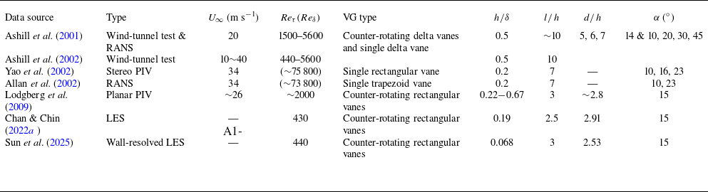
 δ
 h
 l
 d
 α
 Reδ=U∞δ/ν
 U∞
 δ
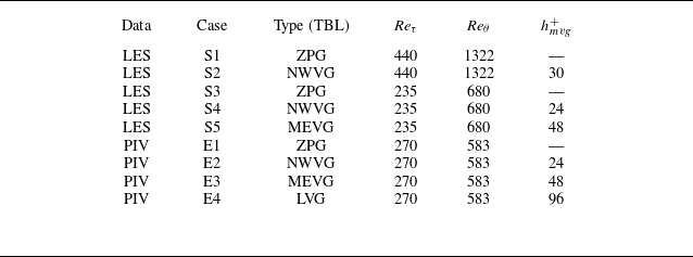
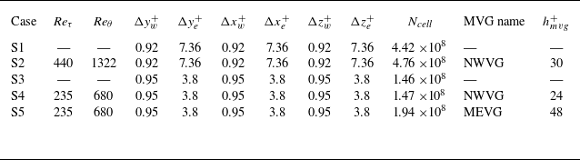
 Reτ
 Reτ
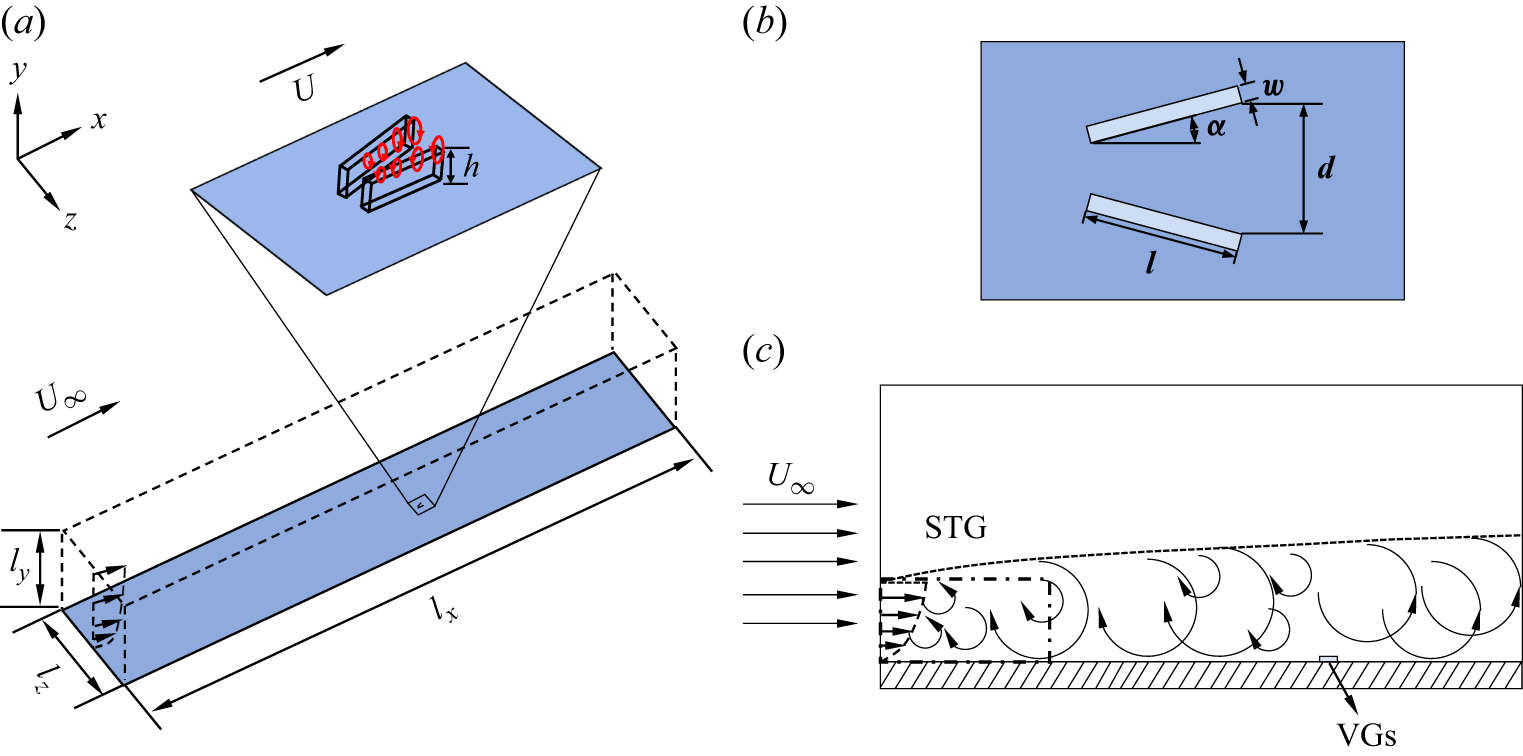
 a
 b
 c
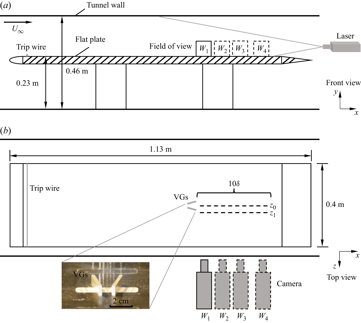
 y−x
 a
 b
 W1
 W2
 W3
 W4
 z=0
 z1=1.5h
 h
 x
 δ
 δ
 W1

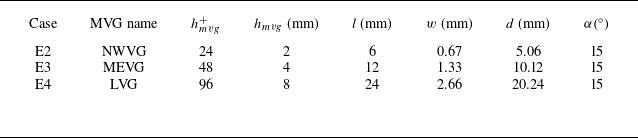
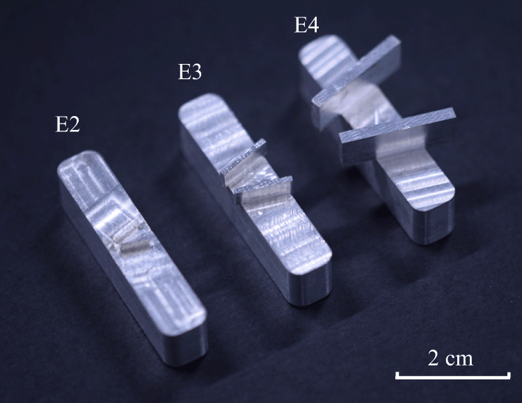
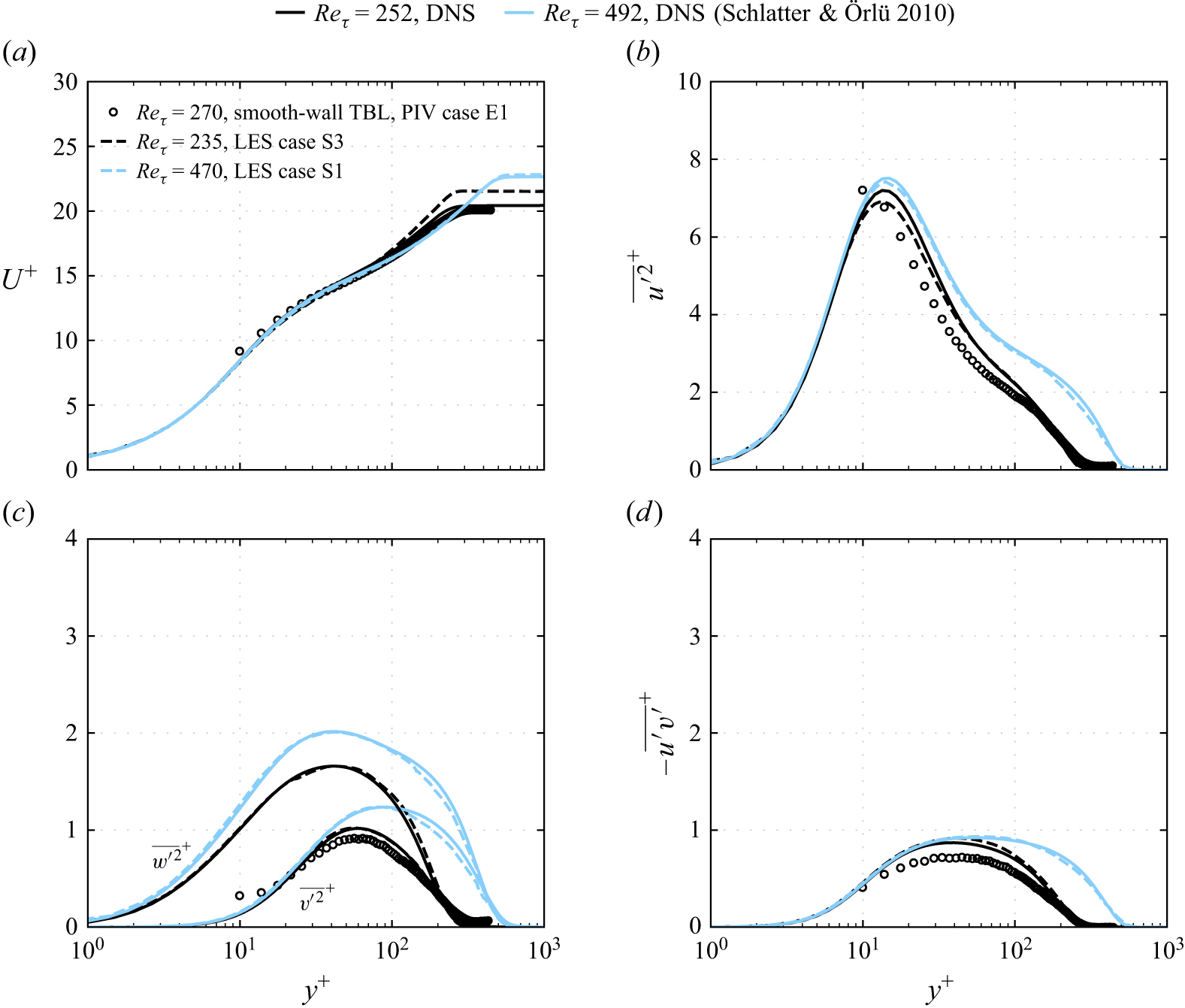
 Reτ
 Reτ
 Reτ

 λ2
 a
 h+=24
 b
 h+=48
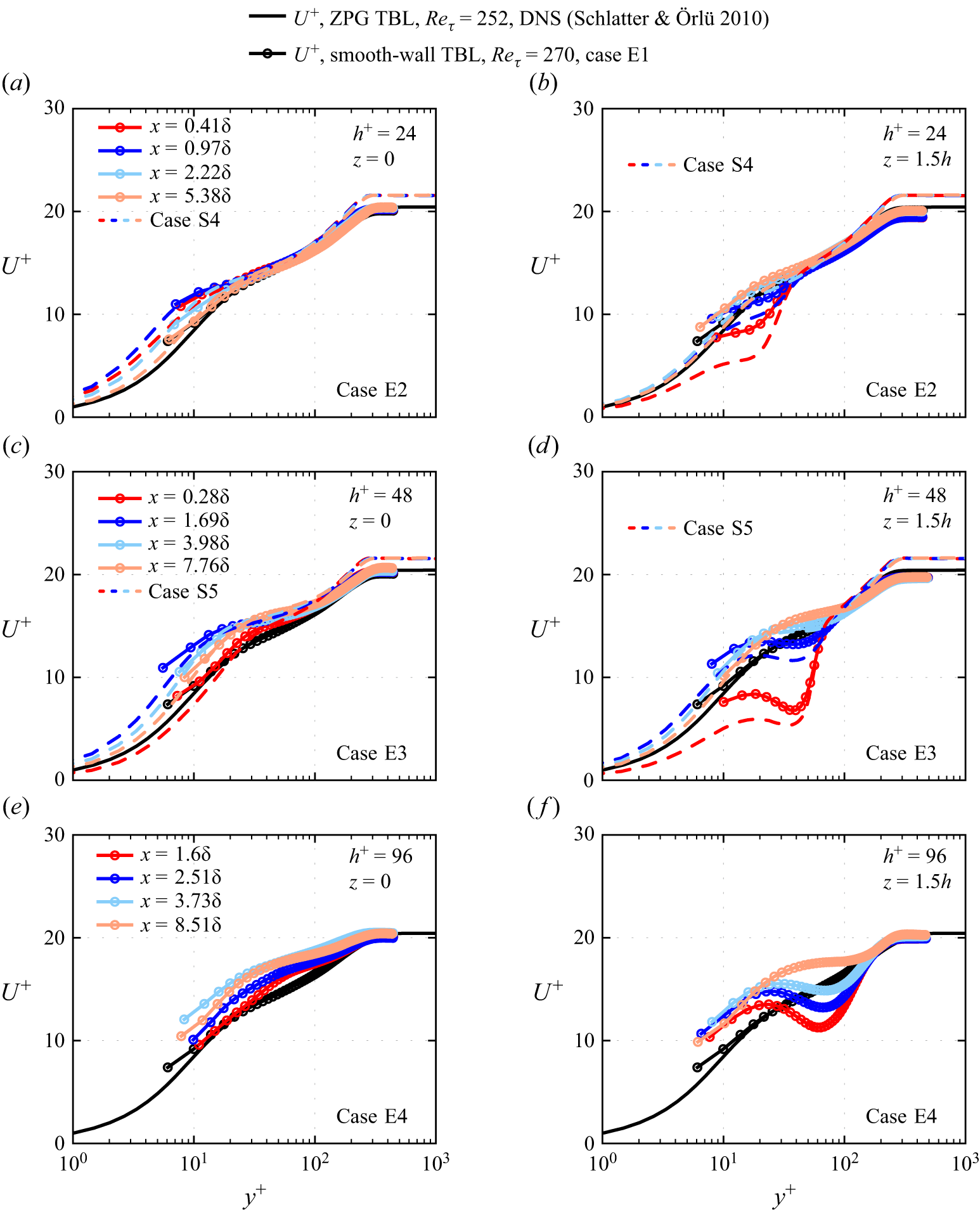
 z=0
 1.5h
 h+
 h/δ
 uτ
 x
 y
 δ
 δv
 uτ
 δ
 δv
 Reτ=270
 Reτ=235
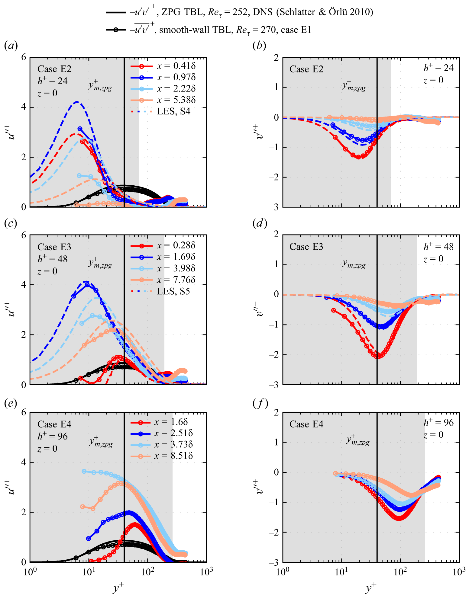
 z=0
 ym,zpg+
 h+
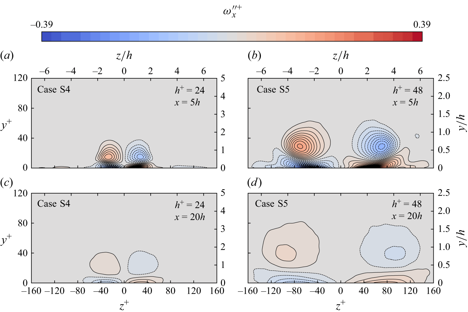
 h+=24
 h+=48
 a,b
 x=5h
 c,d
 x=20h
 y
 z
 h
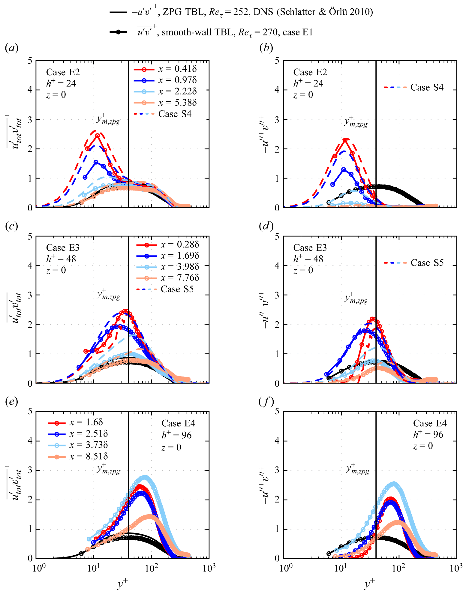
 −utot′vtot′¯
 −u′′v′′
 z=0
 ym,zpg+
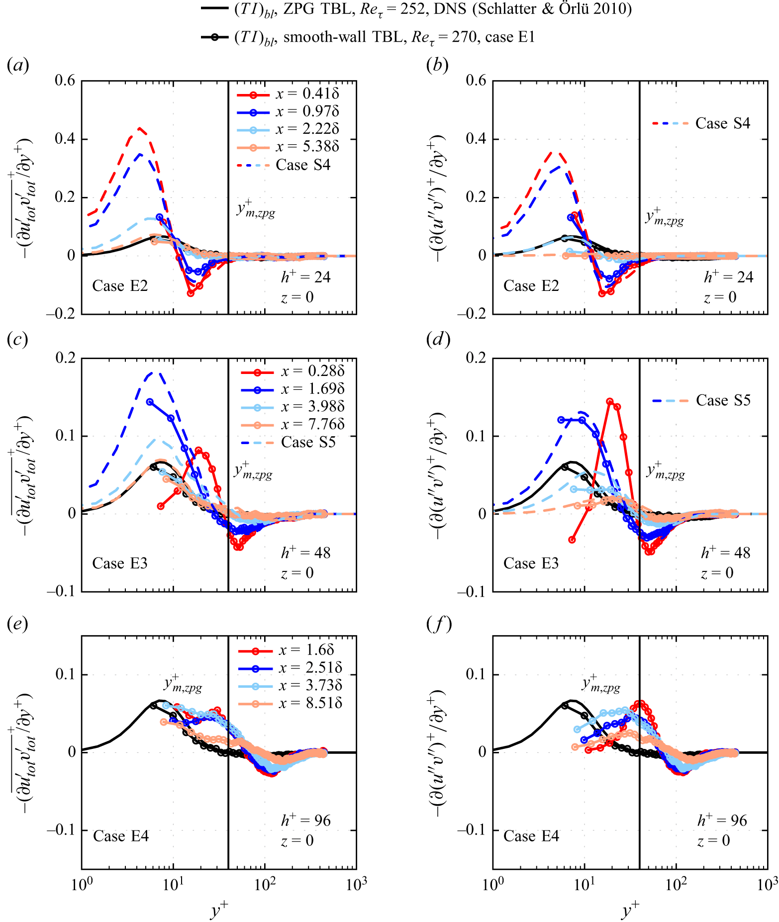
 a,c,e
 (TI)tot
 b,d,f
 (TI)′′
 z=0
 (TI)bl
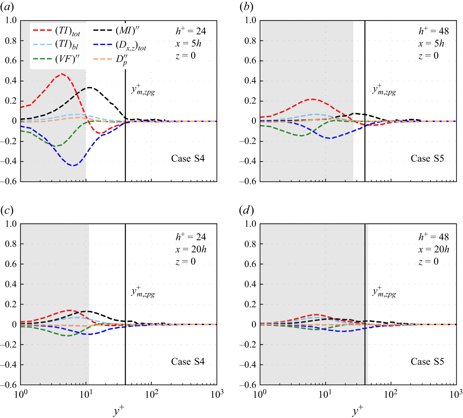
 z=0
 a,b
 x=5h
 c,d
 x=20h
 h+=24
 h+=48
 (TI)tot
 (TI)bl
 (VF)′′
 (MI)′′
 (Dx,z)tot
 x
 Dp′′
 (TI)tot−(TI)bl>0
 ym,zpg+∼40
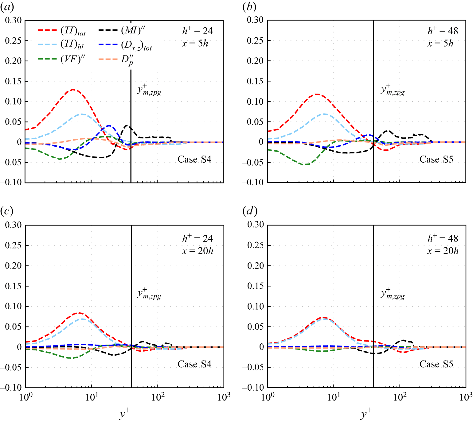
 Δz≈10h
 a,b
 x=5h
 c,d
 x=20h
 h+=24
 h+=48
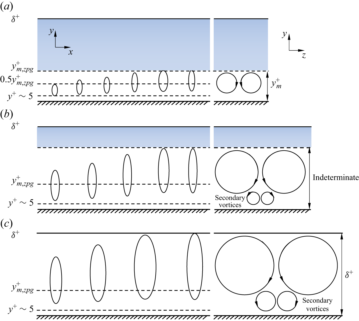
 a
 h+=24
 h+=30
 b
 h+=48
 h+=96
 y
 x
 y
 z
 ym,zpg+
 δ+
 b
 c
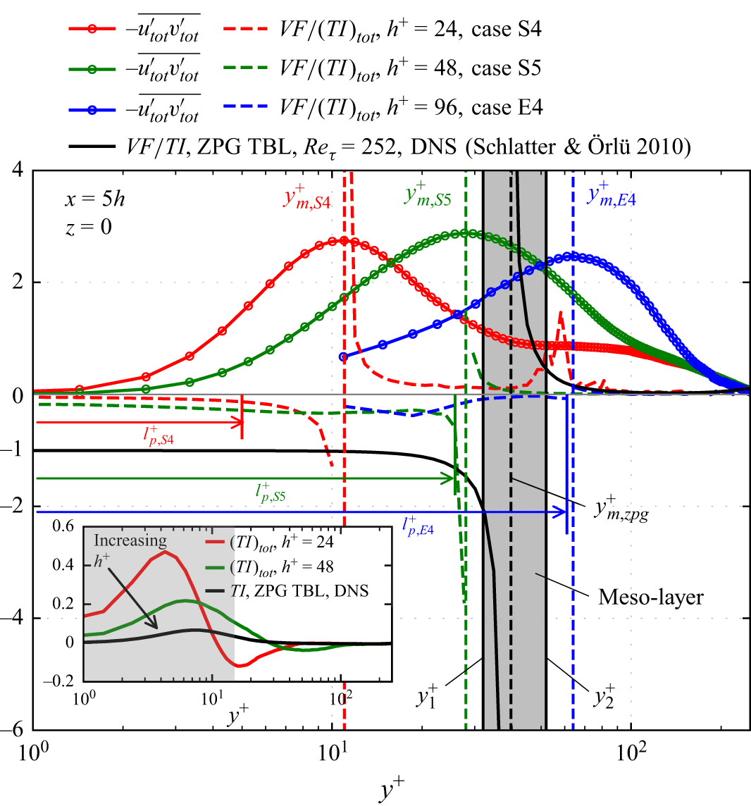
 VF/(TI)tot
 −utot′vtot′¯
 z=0
 x=5h
 VF/TI
 −utot′vtot′¯
 y1+
 VF/TI=−2
 y2+
 VF/TI=0.5
 ym,zpg+∼2δ+
 lp+
 yp+
 VF/(TI)tot
 yp+
 VF/(TI)tot=−0.4
 yp+
 ym,E4+
 (TI)tot
 h+
 VF/TI≈
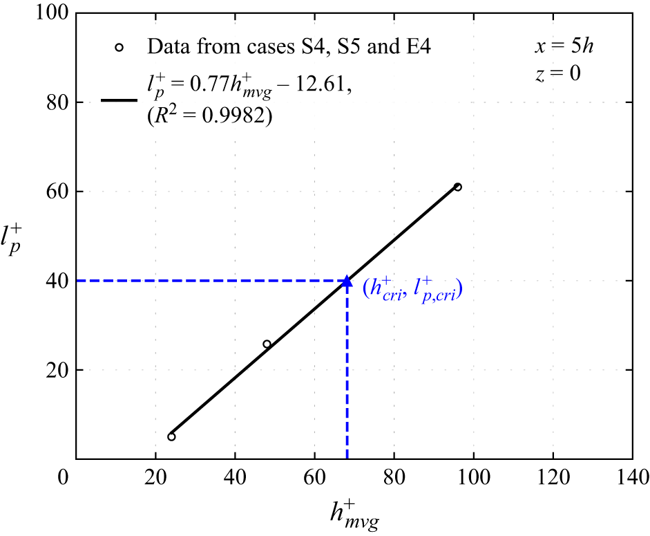
 lp+
 hmvg+
 lp+
 x=5h
 z=0
 R
 95%
 hcri+
 lp,cri+(=ym,zpg+≈40)
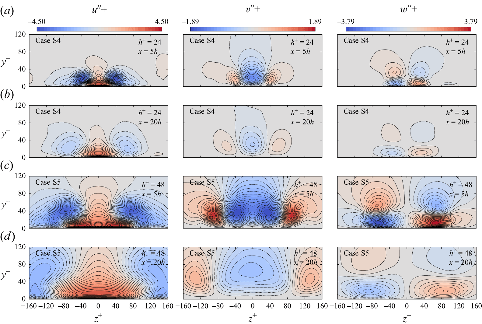
 a,b
 h+=24
 a,b
 c,d
 h+=48
 a,c
 x=5h
 b,d
 x=20h
 y
 z
 u′′
 v′′
 w′′
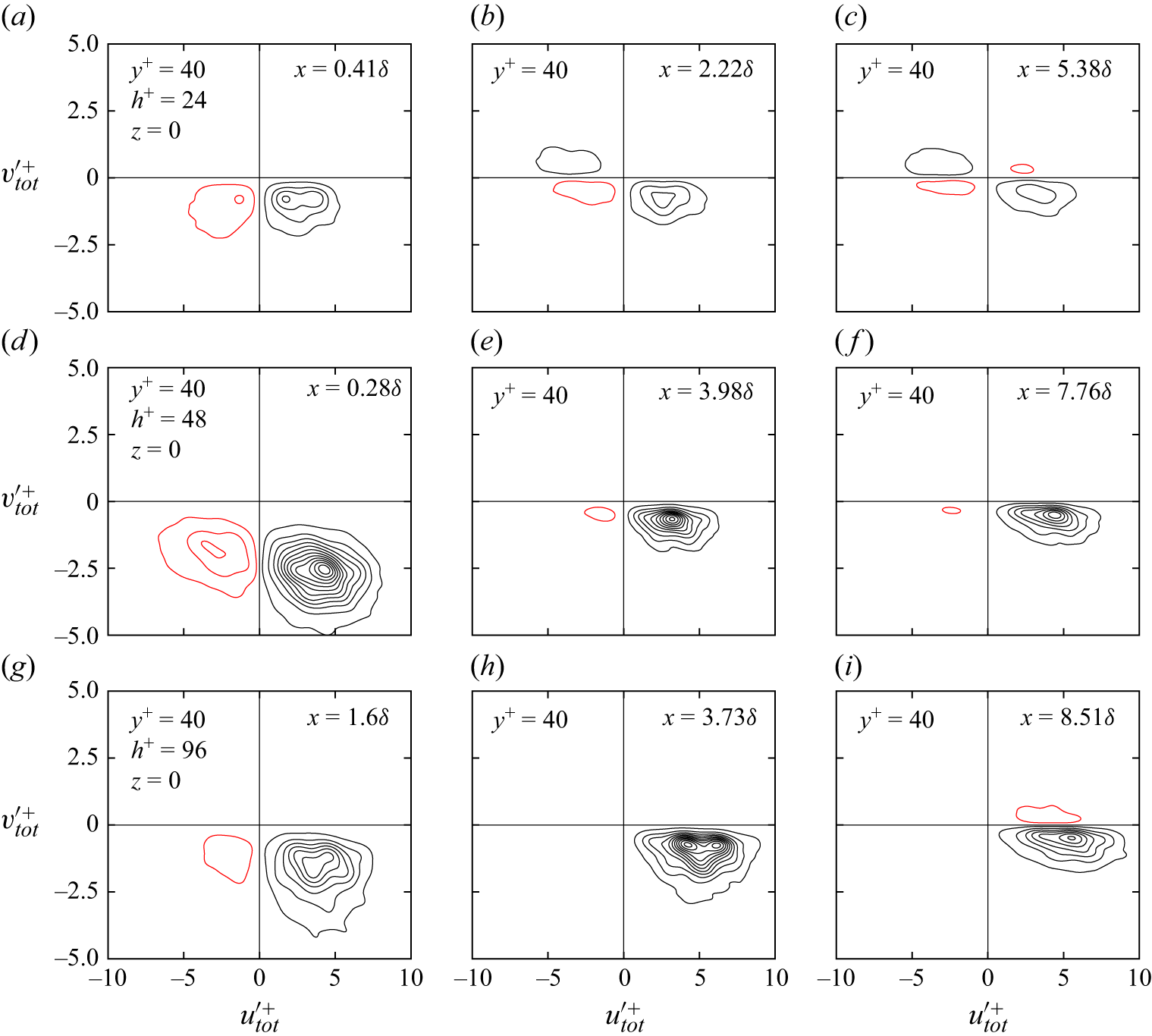
 utot′
 vtot′
 ym,zpg+=40
 z=0
 h+=24,48
 96
 x
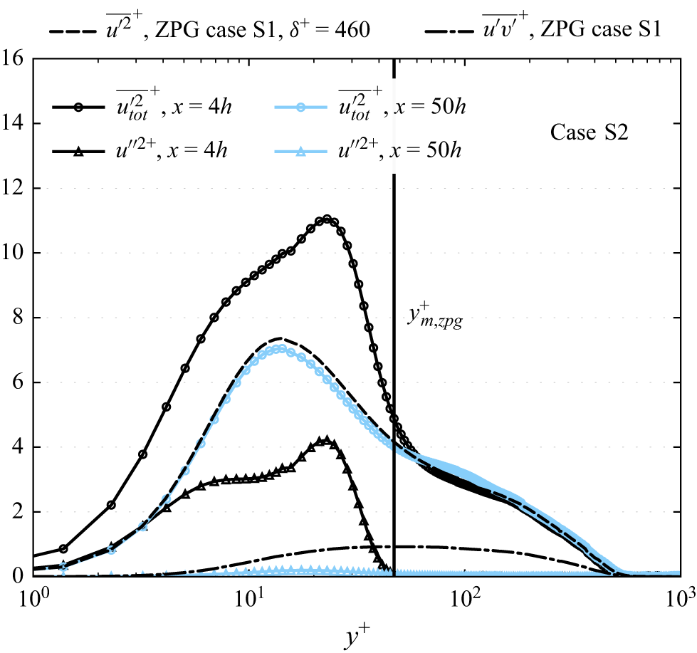
 Δz≈10h
 x=4h
 50h
 utot′2¯+
 u′′2+
 u′2¯+
 −u′v′¯+
 δ+=460
 ym,zpg+≈47
 −u′v′¯+

 Open access

