

1. Introduction
Stresses are nonuniform along fault planes. Stress intensities reach their maxima towards the fault termination zone as implied from fracture experimentation (Lawn & Wilshaw, Reference Lawn and Wilshaw1975). Consequently, fault rupture and growth, secondary faulting and seismic activities are closely associated with fault terminations (Chinnery, Reference Chinnery1966a,Reference Chinneryb; Aki, Reference Aki, Schwartz and Sibson1989; King, Reference King1986); therefore, detailed familiarity with the properties of fault termination zones is essential for the understanding of these phenomena.
Secondary faulting can be considered an extension of the primary fault (Pr), characteristically along planes that deviate in orientation from that of the primary one. We consider here a contractional jog fault termination in which fault segmentation into one or more curved ruptures occurs. Fault terminations have been studied in various scales, shapes and tectonic settings (Ringenbach et al. Reference Ringenbach, Pinet, Stephan and Delteil1993; Couzens & Dunne, Reference Couzens and Dunne1994; Little & Roberts, Reference Little and Roberts1997; Simancas et al. Reference Simancas, Azor, Martinez Poyatos, Gonzalez Lodeiro and Caro1997; Klerks, Theunissen & Delvaux, Reference Klerks, Theunissen and Delvaux1998; Dhont et al. Reference Dhont, Chorowicz, Yurur, Froger, Kose and Gundogdu1998; Bayasgalan et al. Reference Bayasgalan, Jackson, Ritz and Carretier1999; Salvini, Billi & Wise, Reference Salvini, Billi and Wise1999; Kim, Peacock & Sanderson, Reference Kim, Peacock and Sanderson2003; Oskin & Iriondo, Reference Oskin and Iriondo2004; Alik, Mueller & Schubert, Reference Alik, Mueller and Schubert2005). Yet, detailed field characterizations of fault terminations are rare (see e.g. Cruikshank, Shao & Johnson, Reference Cruikshank, Shao and Johnson1991 and references therein). The present study concerns a unique exposure of a fault termination zone from Middle Eocene chalks near Beer Sheva, Israel, which reveals the end of a primary fault, secondary fault segmentation and a joint set genetically associated with the secondary faulting (Bahat, Rabinovitch & Frid, Reference Bahat, Rabinovitch and Frid2005, p. 494).
We use fracture mechanical calculations to estimate the stress field inducing the faulting from the geometry of the fault termination zone. We apply Chinnery's model (Reference Chinnery1963, Reference Chinnery1966a,Reference Chinneryb and references therein) as it provides a very good first approximation.
We have made the following rather crude approximation. The changes brought by the time development of the secondary fracture upon the total stress field are ignored and all the secondary fracture evolution is based on the field caused by the Pr. The motivation for such an approximation is twofold: (1) the secondary fault (S1) is of a smaller length than the Pr and hence the total field is not supposed to be significantly influenced by the former; (2) the time interval of the secondary fault propagation is assumed small compared with the stress field adjustment time.
2. Background
Calculations of stress fields in the area of fault termination zones have been carried out by Chinnery (Reference Chinnery1963, Reference Chinnery1966a,Reference Chinneryb), Das & Scholz (Reference Das and Scholtz1982) and Cruikshank and others (Reference Cruikshank, Shao and Johnson1991). Du & Aydin (Reference Du and Aydin1995) simulated shear fracture paths extending from an isolated fault. We adapt Chinnery's method because it relates to a relatively large distance from the edge of the primary fault and covers a section of the first part of the curved fault (S1). Our purpose is to analyse the primary fault and the curved fault, and we found that for this purpose it was reasonably easy to extend Chinnery's method. Moreover, these extended theoretical results best fit our field observations. We examine four possibilities in a contractional jog (versus Chinnery's investigation, which was limited to fracture at 30° in compression and at 45° in extension).
Strike-slip faults commonly occur under the action of uniaxial compression inclined at about 30° to the fault plane. Chinnery (Reference Chinnery1966a,Reference Chinneryb) also considered strike-slip movements in regions of pure shear and extension. Rayleigh & Marone (Reference Rayleigh, Marone, Hobbs and Heard1986) suggested that, ‘ideally’, strike-slip faults are driven to failure by pure shear loading. Bombolakis (Reference Bombolakis, Podwysocki and Earle1976, fig. 4) summarized the four end-member conditions of failure by triaxial tests: fracture occurs in compression at 0° and at 30°, and fracture occurs in extension at 0° and at 45°
3. Field characterization of a fault termination zone of a contractional jog
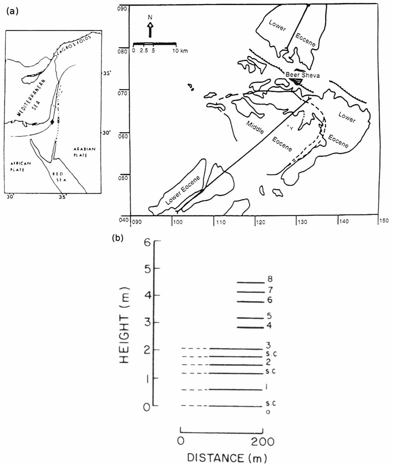
The present study relates to a physical analysis of a fault termination zone that occurs in chalks of Eocene age (Horsha Formation) in Wadi Naim, some 9 km south of Beer Sheva, Israel (Fig. 1a). The termination zone occurs in layer 1 of a cliff marked in Figure 1b, and is mapped (Fig. 2a). The map is a product of a mosaic of 40 photographs partly superposing each other. The combined set of pictures has been photographed from 1 m height at an angle of 90° to the outcrop face (Bahat Reference Bahat1991, p. 275).
(a) Location map at left, rhomb is study area. Area map on the right, showing Beer Sheva at the centre. Curved heavy lines are the boundaries of exposed Eocene rocks and lighter lines (partly dashed) are boundaries between Lower and Middle Eocene formations. Barbed lines are inferred faults south of Beer Sheva. The investigated outcrop at Y. (After Bahat, Reference Bahat1987.) (b) Middle Eocene horizontal chalk layers in outcrop Y. Indurated chalk layers are marked by numbers. Soft chalks (s.c.) alternate with indurated chalk beds in the platform near the base of the exposure. Dashed lines indicate that the platform beds are slightly discontinuous near outcrop. (After Bahat, Reference Bahat1987.)

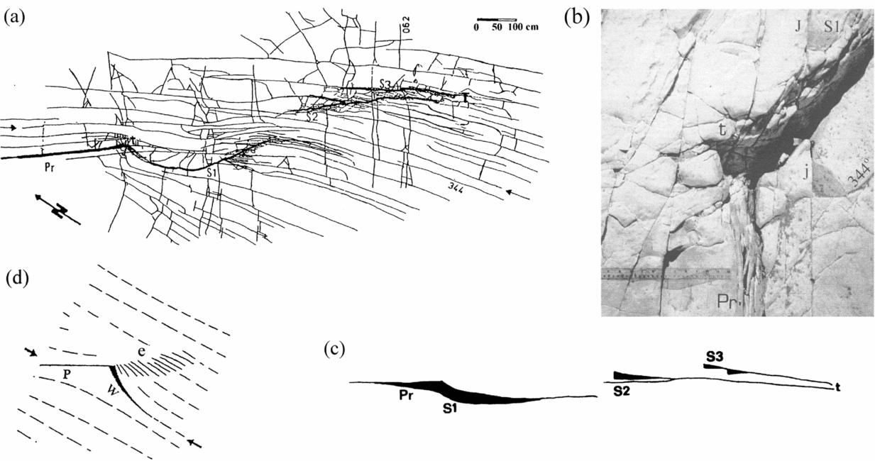
(a) Map of various components of the fault termination zone in layer 1: the primary fault Pr, three segments of the secondary faults S1–S3, and termination at T. The thin lines, which show joint set 344° that crosses the termination zone, change strike close to Pr and S1. (b) Photograph of the end of primary fault Pr, where at its tip t, S1 starts curving. The gap is in the black shadow underneath S1. J and j are joints that belong to set 344°, which changes strike at various locations in the termination zone. The right end of the ruler of 30 cm almost touches the gouge zone along Pr. (c) A perspective scheme of the primary fault Pr, the three en échelon segments (S1–S3) of the secondary fault and the fault termination at T. The vertical displacements along Pr and the three en échelon segments are shown by black areas. Note the rhythmic maxima in S1, S2 and S3. (d) Compression applied at a small angle to primary fault P (arrow), resulting in secondary fractures w and e. The secondary fracture w resembles the initiation of S1, and e resembles the en échelon set S1–S3 in (c) (modified after Petit & Barquins, Reference Petit and Barquins1987, Reference Petit and Barquins1988).

The fault under investigation is a left-stepping bend with right-lateral shear that produced a contractional (anti-dilational) jog. The maximum displacement in the middle of the strike-slip fault transformed into other manifestations of strain around the tip of the fault, where the slip approached zero (e.g. Muraoka & Kamata, Reference Muraoka and Kamata1983). Such changes often lead to a complex geometry in the fault termination zone, including jogs, bulging, secondary faults, joints and bending in the fracture components (e.g. Trudgill & Cartwright, Reference Trudgill and Cartwright1994). In this particular case, failure in the weak chalk has resulted in a unique combination of a primary fault and eight secondary structures (Bahat, Reference Bahat1991, p. 275; Bahat, Rabinovitch & Frid, Reference Bahat, Rabinovitch and Frid2005, pp. 494–503).
We consider the approximately straight fault striking 317° (Pr in Fig. 2a) to be the exposed part of the primary fault. The extent of the fault continuation towards the northwest into the cliff is not known. The southwestern side of the fault was downthrown in relation to the northeastern one.
The primary fault is followed at its end by a series of three fault segments that constitute a left-stepping en échelon set (S1–S3, Fig. 2a). The secondary faulting, together with the end of the primary fault, describes the fault termination zone.
The first segment (S1) is curved with its concave side towards the northeast. Combined with the primary fault, it forms a sickle shape. This is the segment that we fitted with our calculations.
A second segment (S2), which is slightly concave towards the southwest, overlaps about 0.6 m of the first segment and terminates at its southeastern end (T). At its northwestern end the segment has a splay about 70 cm long. There is a third segment (S3), which is almost straight and its entire length overlaps the second segment. The end of the third segment is assumed to be the fault termination location (T in Fig. 2a). The distance between the third and the second segments varies from about 40 cm at their northwestern ends to about 15 cm at their southeastern ends. The straight chord lengths (ignoring curvatures) of the three segments are 3.7 m, 3.9 m and 2.9 m, respectively.
There is a gap between the fault walls that continues laterally along S1 (Fig. 2b). There are some gouge remnants of secondary material in this area, suggesting that possibly more material had filled the gap before being washed away. The gap is irregular and its reconstruction to its original condition may be achieved in two alternative ways.
The rock is considerably ruptured into splinters that range in size from several centimetres to several millimetres along the en échelon segments (mostly between the second and third segments). There is a component of vertical displacement along these en échelon segments. The offset is generally maximal at the northwestern part of each segment and it vanishes towards its southeastern end. The maxima of vertical displacement along the three en échelon segments are 15 cm, 8 cm and 6 cm, respectively (Fig. 2c). The offsets occur along vertical planes, and in all places the southwestern side of the fault moved down with respect to the northeastern side. Opening of about 1 cm is observed along major parts of the three en échelon segments.
The joint set 344° is spatially confined on both sides of the fault in a zone some 7 m wide in layer 1 and does not appear elsewhere in the Wadi outcrop. It is bounded along the northeastern side by talus, and along its southwestern side it has contacts with a joint set oriented at 028° in a manner implying that set 028° is younger (Bahat, Reference Bahat1987). Both sets are cut by a third fracture set 062°, which has a local extent. A fuller description of this fault termination zone is given in Bahat, Rabinovitch & Frid (Reference Bahat, Rabinovitch and Frid2005, p. 494).
The fault has certain features that resemble a normal fault, like vertical displacement and almost no offsets close to its tip. Nevertheless, this structure is identified as a termination zone of a strike-slip fault for the following reasons (there are no indications of oblique slip):
(1) The gouge zone along the primary fault reaches the width of 7 cm at its tip, and is sheared, resulting in slightly curved left-stepping R-shears (Fig. 2b) resembling the right-lateral shear zones obtained experimentally by Bartlett, Friedman & Logan (Reference Bartlett, Friedman and Logan1981, fig. 6).
(2) Closing of the gap between Pr and S1 (Fig. 2b) can be achieved by two alternative movements: either the downthrown side is brought in contact with Pr by laterally overlapping the shear zone, leaving about 0.5 cm right-lateral displacement along Pr; alternatively, a left-lateral slip of 2.5 cm of the downthrown side along the gouge would close S1 quite well. Thus, both closings would indicate an original right-lateral displacement along Pr and S1, while the latter mechanism is more convincing.
(3) Petit & Barquins (Reference Petit and Barquins1987, Reference Petit and Barquins1988) demonstrated experimental results obtained from polymethyl metacrylate and sandstone under uniaxial compression, creating a ‘wing crack’, resembling the first part of S1, like the fracture geometry in the termination zone in terms of stress direction (Fig. 2d). Furthermore, S1 combined with the primary fault Pr forms a sickle shape very similar to Chinnery's model produced by a strike-slip displacement. The vertical displacements along the strike-slip fault and opening across the en échelon segments compensated for the lack of lateral displacements along Pr (Lensen, Reference Lensen1958).
(4) There were 16 fracture episodes of faulting, jointing and displacements in the termination zone (Bahat, Rabinovith & Frid, Reference Bahat, Rabinovitch and Frid2005, table 6.2), of which, bulging is perhaps the most characteristic phenomenon. There is a gradual increase in vertical displacement from NW to SE along Pr towards its tip from 0 to 10 cm, initiating the bulge. When the lateral offset along Pr was exhausted at around the tip, further stress release resulted in vertical stresses producing bulging of the first part of S1 (Fig. 2b, c), as well as other secondary fractures (more details are given in Bahat, Rabinovitch & Frid, Reference Bahat, Rabinovitch and Frid2005, pp. 494–503).
(5) The three left-stepping en échelon fault segments (Fig. 2a) reflect a right-lateral shear.
(6) The almost lack of interaction of joints of set 344° suggests a major stress coaxial to the strike of the joints (Bahat, Reference Bahat1991, p. 320). This supports our model of a lateral stress at 26° to the primary fault.
(7) In a strike-slip contractional jog, a vertical upthrow along one side of the fault would occur in the compressional regime and a downthrow would occur in the tensional one (Chinnery & Petrak, Reference Chinnery and Petrak1968). Accordingly, bulging along the primary and secondary faults is exhibited in the upthrown block (Fig. 2c) as observed in the termination zone. The rhythmic maxima in the vertical displacements along S1, S2 and S3 imply that these bulges occurred concurrently with each individual fault. A single vertical displacement of normal faulting at a later time would be expected to have been monotonous with a gradual change from maximum to minimum throughout the termination zone rather than a rhythmic one. This rhythmic mechanism suggests an incremental growth of the secondary faults with each lateral stress.
(8) Our calculations resulted in almost pure lateral shear supporting the strike-slip assumption.
4. The model
We assume that the remote stress field direction did not change during the complete sequence of the fault termination process, but its amplitude was repeatedly modified, thus producing the secondary features. Our analysis is based on the shape of S1, limiting our calculations to the conditions associated with the lateral strain in the termination zone. The calculations are an adaptation of Chinnery's (Reference Chinnery1963, Reference Chinnery1966a) model. They are based on the following method. The exact shape of the secondary fault (S1, Fig. 2a) is assumed to be dependent on (1) the initial stress field τ 0, which created the primary fault Pr, (2) the stress change τ 1 due to the faulting, and (3) the exact point of initiation of the secondary fault. The field τ 1 in turn depends upon the geometry of Pr and upon the Lamé constants of the rock involved. Several parameters are known while the unknown parameters are varied within reasonable ranges. For each set of such parameters the shape of S1 is calculated. The parameters which give the best fit to the observed shape of S1 are supposed to be the correct ones.
We assume that Pr was caused by an initial uniform stress field τ 0. Throughout this work we apply the convention that positive stresses denote compression, while negative ones denote tension. This is in contrast to Chinnery's convention. The stress field τ0, using its principal axes σ 1 and σ 3 (σ 1 > σ 3) and neglecting the vertical σ 2, is given by:

The principal axes are assumed to be in the following conventional directions: the first, σ 1, is parallel to joint set 344° (assuming coaxiality of the set with the maximum horizontal principal stress σ 1) and horizontal with approximate error of ± 5° (Figs 2a, 3). The second, σ 3, is perpendicular to the first and is also along the Earth's surface, and the third, σ 2, is directed vertically downwards.
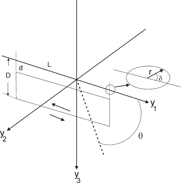
Model of the primary fault: 2L, d, D are the fault's length and the fault's depths. In our calculations we assume d = 0. Inset: sign convention for δ.

Pr is assumed to be of a rectangular shape with length 2L and vertical depths d and D (Chinnery, Reference Chinnery1966a) (Fig. 3). The axes y 1, y 2 (horizontal) and y 3 are defined such that the primary fault is in the y 1–y 3 plane. Note that the order of y 1, y 2, y 3 is according to the mathematical convention. The stress σ 1 is tilted horizontally by an angle θ (which is measured counterclockwise) from the positive direction of y 1.
The creation of Pr is assumed (Chinnery, Reference Chinnery1966a) to have relieved locally a partial amount τ 1 of the stress field. At the end of the process, the remaining stress field given by

is the cause for the secondary fault.
The value of τ 1 is calculated by the ‘dislocation theory’ (Steketee, Reference Steketee1958): a nonstressed semi-infinite material having elastic constants λ and μ is cut along the rectangular fault slit shown in Figure 3. One side is moved a distance a with respect to the other and the cut is then sealed. This ‘dislocation’ of slip a creates a stress field of size −τ1, which can be readily calculated (Chinnery, Reference Chinnery1963). A summary of the results is as follows:
Let  denote an arbitrary point, which, due to the ‘dislocation’, experiences a displacement
 and is relocated at
 .
For an arbitrary function f(x 1, x 3) we define

(note that x 1, x 3 are only auxiliary variables) and use this notation to calculate  (Chinnery, Reference Chinnery1966a) by


where

and

Once  is known, the symmetric stress tensor τ1 = {(τ1)ij}, 1⋚i, j⋚3 is given by

All the derivatives in Eq. (9) can be computed numerically using finite differences. Throughout this work computations were restricted to two-dimensional problems in the plane y 1–y 2. Consequently only the entries τ 11, τ 22, τ 12 of τ were considered.
Transforming the initial stress field of Eq. (1) (reduced to its 2D representation) to the y 1–y 2 coordinate system, yields

where θ is the angle between y 1 and σ 1.
5. The calculation procedure
In order to uniquely determine a secondary fault, it is sufficient to specify the parameters L, D, d, a, λ, μ, σ 1, σ 3, θ, y 10, y 20 where (y 10, y 20) is the starting point of the secondary fault. In our case, the angle θ (between 344° and the primary fault direction) is pre-fixed from Figure 3 as θ = 154° ± 5° (−26° ± 5°, see also Fig. 2a). Since it is assumed (Chinnery, Reference Chinnery1966a) that at (0, 0), at the centre of the fault, all shear stress has been relieved, i.e. (τ)12(0, 0) = 0, another unknown parameter is eliminated and the stresses σ 1 and σ 3 can be replaced by a single parameter k = −σ 3/σ 1. The parameter k was chosen between 0.5 and 1, since k < 0.5 led to completely unreasonable S1 (see Section 6). The remaining unknowns are divided into two categories: (1) configuration parameters which affect both the magnitude of τ and the secondary fault's path; (2) scaling parameters which affect the magnitude of τ but preserve the path's shape.
By defining ν = λ/[2(λ + μ)] (Poisson's ratio), ν becomes a configuration parameter while λ remains only a scale parameter (Eqs (8, 9)). Another scale parameter is the displacement a (Eqs (4–6), (9)). We also assume d = 0 (see Fig. 3) and thus one needs to assign values to only six parameters, namely L, D, k, ν, y 10, y 20, in the process of best approximating the secondary fracture's shape.
A reasonable choice for a starting point is the endpoint of the primary fault. However, (L, 0) is a singular point at which Eqs (4–6) expire. We therefore choose (y 10, y 20) as being ‘sufficiently close’ to (L, 0) (Brace & Bombolakis, Reference Brace and Bombolakis1963). Let (r, −δ) denote the polar coordinates of (y 10, y 20) with respect to (L, 0) as an origin (Fig. 3, inset). Note that δ is measured counterclockwise with respect to the positive direction of y 1.
The competitive requests that r be as small as possible but at the same time that the starting point remains outside the singular point (L, 0) where Eq. (9) is not valid, dictated the value of r as 0.1 cm ≤ r ≤ 0.5 cm.
The rock under investigation has the Lamé constants λ = 3.45 × 10⁹ dyn/cm2 and μ = 2.3 × 10⁹ dyn/cm2, i.e. ν = 0.3. These constants were calculated from Koifman & Flexer (Reference Koifman and Flexer1975). The primary fault's dimensions L and D are assumed to satisfy 1000 cm ≤ L ≤ 4000 cm and 50 cm ≤ D ≤ 500 cm. The vertical dimension D of the fault is assumed to cut at least one layer (of the thickness of 60 cm) and possibly several such layers, but it probably does not penetrate to greater depths, as estimated from the appearance of other small faults in the investigated area. The fault length L is approximated to be the general size of the small faults in the investigated syncline.
The numerical procedure was as follows. We first carried out a systematic check to determine the relative influence of each parameter on the shape of S1. We next, for an initial choice of k, varied the remaining parameters sequentially, moving from the most to the least effective parameter (on the shape of S1). For each parameter set we simulated S1 and if the best simulation was not sufficiently close to the real S1, we changed k and repeated the process.
Each simulation consisted of two steps:
Step 1: Starting the path. As previously stated, the secondary fault starts at some point (r, −δ) where r satisfies 0.1 cm ≤ r ≤ 0.5 cm. The choice for δ is also limited (Chinnery, Reference Chinnery1966a) since secondary faulting is ‘very likely’ to be initiated in the region of tension, i.e. where the stress invariant τ 11 + τ 22 is negative. For example, in the particular cases of pure shear (σ 3 = −σ 1) and uniaxial compression (σ 3 = 0), this restriction yields y 20 < 0, 0° < δ < 180° (see Chinnery, Reference Chinnery1966b, Fig. 4). However, throughout this work, we took 45° ≤ δ ≤ 60°. Any other choice tried in the calculations did not generate an acceptable S1 (see Section 6).

Step 2: computing the next point. We assumed that (1) when the ground was in extension, i.e. τ11 + τ22 ≤ 0, failure occurred at an angle of 45° (Chinnery, Reference Chinnery1966a) or 0° (Bombolakis, Reference Bombolakis, Podwysocki and Earle1976) to the principal axis; (2) when the ground was in compression, i.e. τ11 + τ22 ≥ 0, failure occurred at 30° (Chinnery, Reference Chinnery1966a) or 0° (Bombolakis, Reference Bombolakis, Podwysocki and Earle1976) to the principal axis. However, since the angle between the Pr in the present study and σ 1 was ≈ 30° (26° ± 5°), we have assumed that under the conditions here, the only failure direction in compression was 30°.
The implementation of these ‘rules’ defines two possible procedures for constructing the shape of S1. They are denoted by F(45, 30) (used by Chinnery), and F(0, 30), respectively. The first and the second numbers of any of the pairs indicate the angles chosen throughout the regions of extension and compression, respectively.
At each point there may be two forward directions along which the secondary fault may propagate. The chosen direction was that which was closer to the direction of the previous step. Thus, a secondary fault which is continuous and smooth, except at the boundary between regions of extension and compression, is computed. At this boundary τ11 + τ22 = 0 we obtain a jump in the fault's direction.
Step 2 is repeated until the complete secondary fault is simulated. Numerical results are given in the next Section and consist of (1) preliminary testing of the secondary fracture's sensitivity to changes in D, δ, k, ν, and (2) producing the parameter set which best approximates the curved fault of Figure 2a.
6. Results and discussion of model calculations
The computations performed throughout this work strongly indicated that the path of S1 is mostly sensitive to changes in the starting point (y 10, y 20), the vertical dimension of Pr, D, and k. The remaining parameters, L and ν, have less effect on that path. In fact, the fracture is almost independent of L.
Throughout the computations it became evident that the procedure which led to a reasonable computed S1 was F(45, 30). The procedure F(0, 30) (and F(0, 0) as well) provided secondary faults that immediately turn backwards for all δ (Fig. 4; note that the length scale is for r, see step 1), and could not be considered for reconstructing S1.
Fracturing at 45° to the direction of maximum compression in extension mode is rarely discussed, because fractures in rocks in this mode generally occur at 0° to the maximum compression direction. An explanation for this deviation is required. As can be deduced from the geological analysis (Bahat, Reference Bahat1999), faulting in the termination zone preceded other processes in the outcrop. It is quite possible that fracture occurred before full uplift, when the rock was below the water table, i.e. the wet rock was very weak, soft and ductile (G. Hayati, unpub. Ph.D. thesis, Israel Inst. Technology, 1975; Bahat, Rabinovitch & Frid, Reference Bahat, Rabinovitch and Frid2001), and maintained low compressive strength. Buchbinder et al. (Reference Buchbinder, Benjamini, Mimran and Gvirtzman1988) investigated the Horsha Formation and found evidence for shear displacements in these chalks while the rock was still partially lithified. Metals under extension in a ductile state would fracture along the planes of maximum shear (while the angle of internal friction is zero) (Knott, Reference Knott1973, fig. 5.3). Accordingly, an analogy to the behaviour of metals would explain our F(45, 30) result in a wet, soft and ductile chalk.
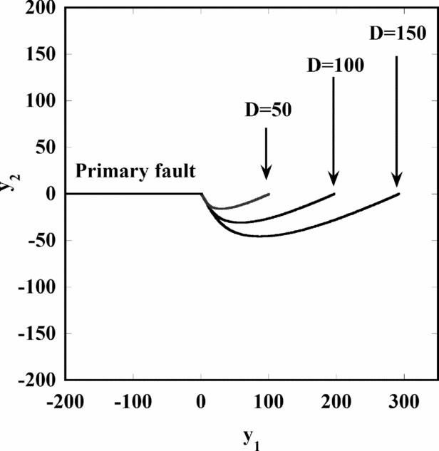
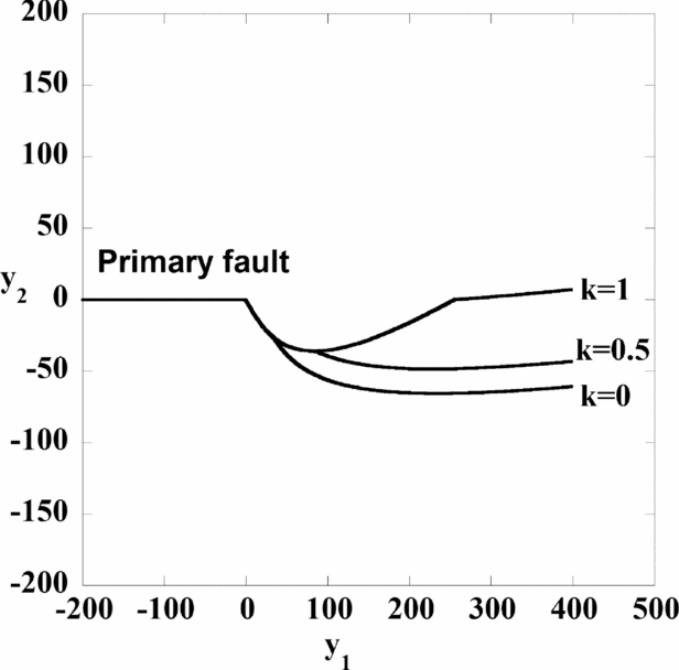
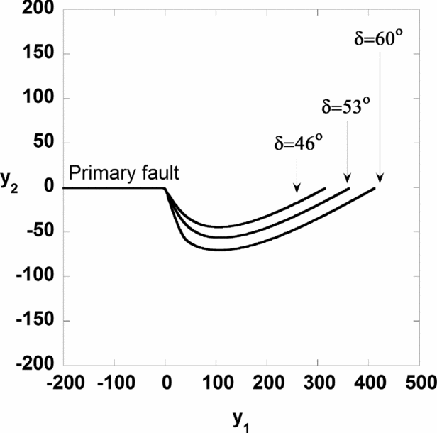
The fracture's shapes for L = 4000 cm, d = 0, θ = 155°, ν = 0.3, k = 1 (pure shear), δ = 53° and various values of D are given in Figure 5. The results for F(45, 30) and F(45, 0) are the same since throughout the calculation we remain in the extension zone. It is seen that the path's length increases almost linearly with D. The effects of changes in k and δ on the path's configuration are shown in Figures 6 and 7, respectively. In both figures we chose D = 150 cm. In Figure 6 one notices an interesting phenomenon: systems with identical parameter sets, except for k, have identical secondary fault shapes for a while before striking off. This follows directly from the basic assumption τ 12(0, 0) = 0, as follows:
The dependence of the computed S1 segment of the secondary fault on the fault's depth D, for L = 4000 cm, d = 0, θ = 155°, ν = 0.3, k = 1 and δ = 53°.

The dependence of the computed S1 segment of the secondary fault on the principal stress ratio k, using F(45, 30) with D = 150 cm, L = 4000 cm.

The dependence of the computed S1 segment of the secondary fault on the angle δ between S1 and the primary fault for D = 190 cm and L = 4000 cm.

At each point, the principal axes of τ = τ 0 − τ 1 are determined by

Since identical parameter sets (except for k) produce identical stress release τ 1, the corresponding secondary faults differ only in τ 0, the original state of stress. However, from Eq. (10) we get

which should be equal to (τ 1)12(0, 0) to model total stress drop. Thus σ 1(1 + k) is independent of k. Also

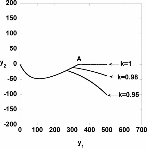
and consequently tan(2ϕ) is independent of k. Therefore, at a given point, secondary faults with different k's but otherwise identical parameter sets will develop identically, as long as the region is either a region of tension or a region of compression (note that τ11 + τ22 is usually different for different k’s). Upon crossing from tension to compression a jump is generated in the fault's direction. The jump's location varies with k (note point A in Fig. 8).
The shapes of curved fault S1 calculated for F(45, 0). The transition between the first and the second parts of the curved fault is at A.

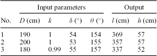
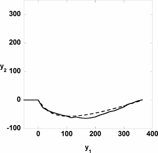
The computer search was conducted as follows. Let l and h denote the y 1 and y 2 projections of S1, respectively. From Figure 2a l should be 370 ± 25 cm while h should be 65 ± 5 cm. A computer search for L, D, k, δ values, which produce a good approximation to the observed fault path, yields L > 1000 cm and several choices of D, k and δ are given in Table 1.
Several parameter sets which approximate the fracture shown in Figure 2a

It should be pointed out that whenever k was less than 0.98 or δ less than 45° or greater than 60°, no computed secondary fracture resembled the one in Figure 2a. The secondary fracture produced by the first parameter set of Table 1 is given in Figure 9.
The best computed shape of S1, calculated by using D = 190 cm, k ≈ 1, δ = 54° and θ = 154°. The observed S1 is given by a solid line. The computed S1 is given by a dashed line.

The exact offset along the primary fault, a, is not known. Note that σ 1 is proportional to a. In assessing the results we need to consider a reasonable range for this parameter. The gouge along the primary fault possibly implies considerable displacement. The observed displacement values close to the edge of the primary fault vary from 0.5 cm to 2.5 cm, more likely the latter. On the other hand the vertical (y 3) displacement at the end of Pr is of the order of 10–15 cm. We propose that this uplift is in fact a transfer of the a movement. A direct displacement in the y 1 direction is impossible owing to the same process which stopped the creation of the main crack (Pr). This displacement (a) was therefore transformed into a displacement in the y 3 direction. Combining the values 0.5–2.5 cm in the y 1 direction with 10–15 cm in the y 3 direction, the offset along the primary fault should have been in the range of 11–20 cm. It appears that the 18 cm vertical displacement along the primary fault, which reflects an element of folding, partially reflects the stored energy involved in the reduction from the assumed displacement of 11–20 cm to the observed displacement of 2.5 or 0.5 cm.
The secondary fault S1 was formed under 45° in extension along its curvy part (Fig. 2a), beyond which it slightly rotated clockwise and continued to propagate sub-parallel to the joints. The propagation sub-parallel to the joints was under 0° in compression. In addition, local changes by 30° (compression) possibly shifted fracture continuation from the end of S1 to the area of S2 initiation. We speculate that the 30° (compression) affected the propagation of both S2 and S3. This compression should explain the angularity formed between the initial S2 (Fig. 2a) and the joints, as well as the fragmentation of the rocks along the stretch between S2 and S3. However, the parallelism between S2, S3 and the joints suggests that the continuation of S2 as well as the full propagation of S3 was mostly controlled by the stress that induced the joints, i.e. 0° (compression) apparently prevailing towards the fault termination.
The magnitudes of σ 1 and σ 3 can be calculated by inserting the values of a, λ and μ in Eq. (9). The relevant parameters used here are λ = 3.46 × 10⁹ dyn/cm2, μ = 2.3 × 10⁹ dyn/cm2, 10 cm < a < 20 cm and L = 4000 cm and the optimal values obtained for Figure 9 are D = 190 cm, k ≈ 1 (almost pure shear), θ = 154° and δ = 54°. The values of σ 1 and σ 3 thus obtained are 3.8 MPa < σ 1 < 7.6 MPa and 3.65 MPa < σ 3 < 7.3 MPa. In our outcrop, since the maximum lateral displacement is unknown, our estimates of σ 1 and σ 3 have but a limited value. For exposures in which the maximal lateral displacement is known, however, our method would yield estimates of the real initial principal stresses.
It is to be noted that Price & Cosgrove (Reference Price and Cosgrove1990), while discussing the previous studies of the formation of secondary fracturing, pointed out the ‘inherent inconsistency’ in Anderson's (Reference Anderson1951) and Chinnery's analyses. We assume that our approach to this problem overcomes that difficulty. We have applied two extensions of Chinnery's techniques. Firstly, we consistently ran the ‘initial point of departure’ method. Secondly, we proceeded incrementally from this point, while the propagation forward from each point depended on the specific trend of the stress field.
The calculations using our modified Chinnery's method show the following two significant results: (1) The obtained direction (54°) of the initial point of departure is in perfect agreement with the field measurement of 50° ± 5°. Moreover, as was pointed out, any different direction values we tried led to vastly different shape forms. (2) The obtained shape of the complete sickle shows almost a full agreement with the curved shape of the secondary fault S1. These results demonstrate the validity of this approach. The calculated stress field, τ, showing almost lateral pure shear fracture conditions, also supports the strike-slip assumption.
7. Summary
An adapted Chinnery method is used to calculate the parameters governing the development of the sickle-like secondary fault for the contractional jog. This method is more applicable than other methods for long distances along the secondary fault and is more readily modified to fit the present calculations; it also agrees well with the present field observations.
From the two conditions that were tested, both F(45, 30) and F(45, 0) procedures lead to a reasonable computed secondary fault, up to the end of the sickle. That is, when the ground is in extension, failure occurs at 45° to the maximum principal axis, while when the ground is in compression, failure occurs at 30° to this axis.
Changes in the overall length, L, of the primary fault and in the Poisson's ratio of the rock, ν, have a small effect on the shape of the secondary fault, while the path is very sensitive to the primary fault vertical dimension, D, to the ratio σ 1/σ 3 and to the initial secondary fault direction, δ.
The best values for the parameters to fit the field data are D = 190 cm, δ = 54° and k = σ 1/σ 3 ≈ 1, which is almost (but not quite) pure shear.
The maximum offset along the primary fault is not known. The observed offset close to the edge of the fault is very small, as expected. The observed vertical displacement in this location is a reasonable substitute for a larger horizontal displacement and is capable of explaining the S1, S3 values and yields an estimation of the existing stresses at incipience. These are estimated to be 3.8 MPa < σ 1 < 7.6 MPa and 3.65 MPa < σ 3 < 7.3 MPa.
Acknowledgment
This study was supported in part by grant No. 91/88 of the Israeli Academy of Science.