

1. INTRODUCTION
There is a large literature within demography and population science analyzing fertility patterns and trends. Within economics, the emphasis is placed on understanding fertility behavior, whereby fertility data is a fundamental ingredient to achieve this goal.Footnote 1 Most “fertility facts,” especially in developing countries, are based on surveys about the reproductive behavior of women, whereas male fertility is largely ignored since most surveys ask only women about their child-bearing behavior. Greene and Biddlecom (Reference Greene and Biddlecom2000) already emphasized this lack of research on male fertility as a problem more than a decade ago, pointing to several specific directions of future research on male reproductive behavior. While this call has stimulated research on the role of men in reproductive behavior (i.e., it is now more common to model reproductive behavior as a bargaining outcome between two partners), the measurement itself has not changed, except for some notable exceptions described below. Because women may remember pregnancies and births better than men, it is often believed that measuring fertility purely based on women’s reproductive behavior is sufficient, and avoids double-counting. In this paper, we seek to question this view by conducting a systematic analysis of gender gaps in completed fertility in a region of the world where these differences are likely to be the largest due to high fertility levels and marriage practices.
Even though each child has two parents, we show that completed fertility rates of men and women need not coincide.Footnote 2 When populations are growing and large age gaps are common, gender gaps in fertility are likely. Such a situation typically goes hand in hand with men fathering children with multiple women.Footnote 3 This could be due to formal polygyny, or simply having children with multiple partners (informal polygyny), which frequently occurs outside of polygynous societies. Another possibility is remarriage after divorce, separation, or death – having additional children with the new partner has largely been ignored in the empirical fertility literature. A traditional household survey only asks women about their reproductive histories and children are rarely assigned to a particular birth father.
There are a few recent notable exceptions of surveys in which men are asked about their reproductive histories. The Survey of Family Growth in the US started interviewing men about their reproductive behavior in 2002. Based on this data, Guzzo and Furstenberg (Reference Guzzo and Furstenberg2007) find that 8% of American men had children with more than one partner. The number among poor African American men is as high as one third, and 16% of them report children with three or more women. Recent waves of the World Values Survey and the Population Acceptance Study also include questions on male fertility, specifically in European countries.Footnote 4 The analysis of administrative register data has become more common in recent years, particularly in Scandinavian countries. Such data typically include information on fathers and mothers. From population registers, it is often possible to construct fertility measures for fathers separate from mothers.Footnote 5 However, this possibility has not been used much in the literature to date.Footnote 6 There is also some related work in demography. For instance, Pison (Reference Pison1986)’s work is close to this paper in spirit and we reach similar conclusions in terms of average male and female fertility. Yet Pison analyzes the marriage market and resulting male–female average fertility differentials for one particular polygynous tribe in Senegal at one point in time.Footnote 7
In sum, what is lacking are attempts to explore systematically the extent to which conventional “fertility facts” would be different if measured based on data from men rather than women. To fill this void, we analyze gender gaps in average fertility, fertility inequality, desired fertility, and demographic transitions across Sub-Saharan African countries. We look at recent waves of the DHS. Starting from the early 1990s, DHS surveys often include a sample of men who are asked about their reproductive behavior.Footnote 8 We select eight countries based on sample size, i.e., those with the largest male samples. To analyze whether there are any robust patterns across countries, we conduct the same analysis in each country. For each country, we piece information together from different waves of the DHS to compare the completed fertility of men and women of the same birth cohort.
We document some striking facts. First, we find that on average men have more children than women of the same cohort in seven out of the eight countries considered. The gaps are large, ranging from 0.8 children in Zambia to 4.6 children in Burkina Faso, but appear to be decreasing over time. For example, in Burkina Faso, we find a gap of 4.6 for the 1944–1948 birth cohort and a smaller gap of only 2.8 for the 1951–1955 birth cohort. Similarly, the gap in Malawi is 2.1 for the 1946–1950 cohort, falls to 1.7 for the 1950–1954 cohort and further decreases to 1.1 for the 1956–1960 cohort. Positive gaps mean that men are bearing children with younger women on average, and that either a larger fraction of women relative to men remains childless or men are bearing children with multiple women. If men reproduce with women who are on average younger and population size is growing, gender gaps in completed fertility will necessarily be positive. Indeed, we find that the size of the gap is positively related to the gender gap in the age of first birth and the degree of formal polygyny.
Second, we document a larger heterogeneity in fertility outcomes among men than among women. The coefficient of variation (CV) of fertility for women is lower than that for men in all countries we analyze, except one cohort in Malawi. In other words, with the exception of this one cohort, women are more similar to each other in their reproductive behavior than are men. The gap is largest in the high polygyny countries Burkina Faso and Benin. Third, we find that differences in the desire to have children can be explained to a large extent by differences in realized fertility. Fourth, we document that the demographic transition started earlier and was steeper when considered from a male perspective.
We believe that these findings are important for a number of reasons. First, investments in children heavily depend on the resources of fathers. There is a large body of the literature investigating how inequality becomes amplified through endogenous fertility and child investments.Footnote 9 The literature shows that it matters how children are spread across families. Given that a large fraction of wealth worldwide is owned by men, it matters how children are distributed across men specifically. In other words, since men control the majority of resources, the number of siblings who share the same father may be more informative than the number of siblings who share the same mother.Footnote 10 A related complication that arises from the fact that men frequently have children who live outside of the household is that the typical assumption that parents’ investment in children can be captured by expenditures on children living in the household is no longer valid. This can lead to inaccurate measurement in the amount that parents invest in their children when living in multiple partnership settings. Fathers’ investment in children will be systematically underestimated when their offspring live in multiple households.
Second, it is often emphasized that men desire more children than women (Bankole and Singh, Reference Bankole and Singh1998). Such discordant preferences are thought to lead to conflict and are sometimes modeled as a bargaining game between spouses (Rasul, Reference Rasul2008; Doepke and Kindermann, Reference Doepke and Kindermann2013).Footnote 11 However, our results show that differences in demand for children are often mirrored in differences in actual achieved fertility, such that there is no innate contradiction surrounding fertility behavior within couples.
In the next section, we describe our data. In Section 3, we document the extent to which average completed fertility differs by gender. Section 4 analyzes differences in fertility inequality for men versus women. In Section 5, we analyze differences in desired fertility and how it relates to actual fertility. Section 6 reconsiders the demographic transition from a male perspective, and Section 7 concludes. The Appendix contains additional data and a simple model.
2. THE DATA
2.1. Some Preliminaries
To analyze fertility behavior of men versus women, we compare “completed fertility rates” (or children ever born) based on self-reported fertility histories.Footnote 12 When using this measure to compare completed fertility rates over time, one usually compares children ever born by birth cohorts of mothers. We follow the same approach here, computing completed fertility rates for men by birth cohorts and comparing them to women of the same birth cohort.Footnote 13 Although men and women of the same birth cohort do not typically have children with each other, the purpose of the paper is to investigate the extent to which cohorts of men and women born at the same time and living during the same years (and hence facing the same economic conditions over their lifetime) differ in their fertility behavior.
The main challenge we face in documenting male fertility is setting the appropriate age cut-off since men can in theory bear children late in life. To ensure that respondents had truly completed childbearing, one would need to use data from relatively old men. However, using data from, say, 70-year-olds in countries where life expectancy is around 50 introduces important concerns about selective mortality. Furthermore, the oldest men included in the DHS, of which we make use, are 59 and the oldest women are 49. Given that constraint, wherever possible, we measure completed fertility based on men aged 55 to 59 and women aged 45 to 49. Thus, one important caveat is that our analysis is unable to capture children born late in life, which biases downward our measures of fertility. This bias will be larger for men than for women.Footnote 14
To compare men and women of the same birth cohort, we have to piece together information from different survey years. For example, we can construct male fertility for the 1941–1945 cohort of men by using 55–59 year-old men from a 2010 survey. If we used the oldest women from the same survey (45–49 years old), they would correspond to a different birth cohort. However, we can use data from a second survey (ideally 2000) to compute the completed fertility rate for the 1941–1945 female cohort by analyzing 45–49 year-old women from the earlier survey. Unfortunately, the DHS surveys are not always spaced exactly 10 years apart. Therefore, we sometimes have to use slightly different ages in our comparisons. The exact combination of data sets, ages, and cohorts used in our analysis will be detailed further below.
2.2. The DHS Samples
We focus on Sub-Saharan Africa and use recent waves of the DHS for our analysis. We picked eight countries based on data availability.Footnote 15 Concretely, our analysis contains those eight countries in Sub-Saharan Africa with the largest male samples and for which a female sample that can be matched with it is available. This leads us to analyze the following eight countries: Benin, Burkina Faso, Ethiopia, Madagascar, Malawi, Rwanda, Zambia, and Zimbabwe.
The spacing between consecutive DHS waves in the same country is typically 5 years, although there are exceptions. Each survey is a representative sample of households.Footnote 16 To assure representativeness on national, regional, and residence levels, individual sample weights are included, which we use in our calculations unless otherwise noted.
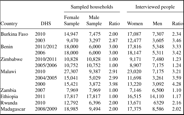
Even though the DHS is a household survey, not all household members are interviewed. The main target group are women of reproductive age (15–49 years). However, recent waves also include interviews with a sub-sample of men (aged 15–54/59). The fraction of men interviewed varies by country and year, with the fraction of households eligible for male interviews varying from around every 1.6th to every 4th household. The final ratio of interviewed women and men also differs due to (small) differences in non-response rates by gender.Footnote 17 The sex ratio of interviewed people for the surveys used are given in Table A2 in the Appendix.
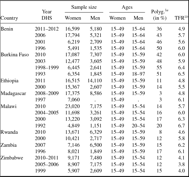
In each of the eight countries, we use all DHS waves that include a male sample with at least 3,000 males. Depending on the country, there are either one (Madagascar, Rwanda, Ethiopia, Zambia), two (Burkina Faso, Benin, Zimbabwe), or three (Malawi) waves that include a large enough male sample. When available, we incorporate an additional earlier wave with only female interviewees, since, as explained above, we use women from earlier surveys to construct the completed fertility rates of the same birth cohorts of men and women. In Table 1, we provide an overview of the surveys used.Footnote 18 The table includes sample sizes by gender and the age ranges of the interviewed people. For the majority of countries, the most recent waves of the DHS were conducted in 2010 or 2011. Only for Madagascar and Zambia was the latest data collected in 2008/2009 and 2007, respectively.
DHS information

Notes: Individual sample weights are used for the calculations. (1a) Polygyny is measured as the fraction of all women, who are married or live together with their partner, with at least one cowife, taking out the missing values. (1b) Total fertility rates are taken from the statcompiler which is based on the corresponding DHS data.
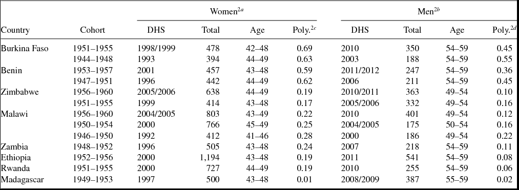
Table 1 also includes the polygyny rates – measured as the fraction of all married women with at least one co-wife – and the total fertility rates (TFR). It is worth noting that our definition of polygyny only considers men who co-reside with multiple women, and does not account for men who co-parent with multiple women living in different households. The highest polygyny rates can be found in Burkina Faso (55% in 1998/1999) and the lowest in Madagascar (3% in 2008/2009).
As explained before, the goal is to compare the number of children ever born by birth cohorts of the parents. Combining men born within a given period of 5 years into one birth cohort ensures sufficiently large sample sizes. For the reasons discussed above, whenever possible we use men between the ages of 55 and 59 and compare them to women aged 45 to 49 from a survey conducted 10 years earlier.
Table 2 provides an overview of which birth cohorts we actually use, from which DHS the information is taken and the respondents’ ages at the time of the interview. We have ordered the countries by their degree of male polygyny, putting Burkina Faso first and Madagascar last.Footnote 19 Note that the (female) polygyny rates reported in Table 2 are higher than those in Table 1 for most countries. This is unsurprising, since the rates in Table 1 also include younger women and people become more polygynous as they age (and polygyny has been falling over time). The table also includes the sample sizes of the relevant birth cohorts, which are obviously much smaller than the size of the overall surveys given in Table 1. Note that we used surveys only around 5 years apart to construct data for the same birth cohorts of men and women in the cases of Malawi and Zimbabwe, given that men were included only up to the age of 54 in these countries, while the oldest women in the survey are 49. Comparing surveys 5 years apart leads to the oldest men and women respectively being from the same birth cohort.
Summary statistics
Notes: Individual sample weights are used to calculate the statistics. (2a) Information is based on the sample of women who provide information on the number of born children. (2b) Information is based on the sample of men who provide information on the number of born children. (2c) Polygyny is measured as the fraction of women who are married or live together with their partner with at least one cowife. (2d) Polygyny is measured as the fraction of men with more than one wife/partner.
The second reason why we cannot always compare exactly 45–49 year-old women to 55–59 year-old men is that the spacing between the surveys is rarely exactly 5 or 10 years. Our procedure here was to use the oldest men for which data is available and adjust the ages of the women so that they are from the exact same birth cohort. This logic explains why the women of the 1951–1955 cohort in Burkina Faso are aged 42–48, for example, given that the DHS are 11–12 years apart.Footnote 20 Fortunately, the surveys include a question on the year of birth, upon which we base our selection of men and women. However, depending on the exact birth date and the month of the survey, 5 years of birth cohort can include people of more than 5 different ages, as the example of Burkina Faso shows. The final sample sizes are obviously much smaller than the size of the surveys. They range from 394 (Burkina Faso DHS 1993) to 1,194 (Ethiopia DHS 2000) for women and from 175 (Malawi DHS 2004/05) to 541 (Ethiopia DHS 2011) for men.
3. GENDER GAPS IN FERTILITY
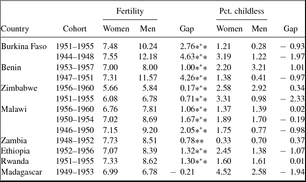
We now compare the average completed fertility for men and women of the same birth cohort. As Table 3 shows, men have many more children than women in almost all countries that we consider. The gap is particularly pronounced in countries with high levels of polygyny. In Burkina Faso, men born in 1944–1948 had on average 12.18 children, compared to only 7.55 for women. The data look similar for Benin, another high polygyny country. Men born in 1947–1951 have on average 11.57 children, while women of the same cohort have only 7.31 – men have on average 4.26 more children than women of the same cohort.
Average completed fertility by gender
Notes: Fertility is measured by the average number of children born to the cohort, considering also men and women with no children. The significance levels are denoted by ***1%, **5%, and *10%. The means are tested on equality based on a two-sample t-test with sampling weights.
The gaps are smaller but positive and significant in all countries but Madagascar. Madagascar depicts the only negative gap, but it is not statistically significantly different from zero. Note that Madagascar is essentially a monogamous country. As Table 2 shows, only 1% of women are in a polygynous union. A positive relationship between polygyny and gender gap in completed fertility is more generally true, as Figure 1 shows. The correlation between the (male) polygyny rate and the gender fertility gap is 0.86. The figure includes a fitted regression line with an R 2 of 0.73. Finally, for those countries where we have multiple cohorts to compare, we see that the gender gap in completed fertility is falling over time. For example, while in Burkina Faso, men of the 1944–1948 cohort had 4.6 children more than women of the same cohort, this gap had fallen to 2.8 for the 1951–1955 cohort. Similarly, the gap for the 1946–1950 Malawian cohort is two children and falls to one child just 10 years later. Benin is the starkest example, where the gap falls from 4.3 to 1 child between two cohorts not even 10 years apart.
Gender gap in fertility versus male polygyny rate.
The data can be used to check how reasonable our assumption of completed fertility at ages 50–54 for men and 42–45 for women is. We do this by calculating the fraction of children below the age of one by age. Details are given and discussed in Appendix A.1. We find that very few women aged 45 or older have any children below one in the household. The numbers for men are somewhat higher, making it difficult to argue that men have truly completed their fertility by age 54. However, this finding biases our results concerning average male fertility downwards. Gender gaps in fertility would be even larger if one could measure true completed fertility.
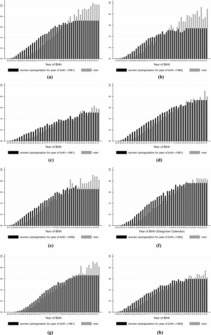
Men achieve these high completed fertility rates by continuing to have children beyond their mid-40s, at ages when women are essentially no longer fertile. To observe this, we depict the number of children born over the life-cycle. Since the DHS are not panels, but rather consist of repeated cross sections, we cannot compute fertility rates for the same cohorts over their life-cycle. Instead, we construct an artificial life cycle by piecing together different cohorts.Footnote 21Figure 2 depicts one life-cycle profile for each country, based on the most recent DHS wave in each of our eight countries. To make it more transparent how these graphs were constructed, we have labeled them with the birth cohort of the mothers and fathers, respectively. To convert the birth years into ages, note that these profiles start at the age 15 and continue to 59 for men in all countries apart from Zimbabwe and Malawi, where the highest age is 54. Furthermore, for women, we have data only until the age of 49. However, female fecundity after the age 49 is essentially zero. Thus, to make the increasing gap between men and women at older ages more visible, we have added figures for the older cohorts of women to the graphs by assuming that fertility does not grow after the age of 49.Footnote 22
Number of children born by birth cohorts. (a) Burkina Faso. (b) Benin. (c) Zimbabwe. (d) Malawi. (e) Zambia. (f) Ethio. (g) Rwanda. (h) Madagascar.
The first thing to note from Figure 2 is that men start having children later in life than women. Accordingly, young women have more children than young men, which is true in all countries that we consider. For example, in Burkina Faso, women in the 1986 cohort, i.e., those aged 24 when asked about their children, already have two children, whereas men of the same age have less than one child on average. However, the gap closes as age increases, which is of course unsurprising given the age gap in marriage. What is more interesting is that the gap eventually reverses sign. In other words, men continue to increase their fertility well into their 50s, while women stop in their mid-40s. This pattern is most pronounced in Burkina Faso and Benin, the most polygynous countries. We can see a similar pattern in the other countries, albeit to a lesser degree.
3.1. The Importance of Population Growth, Mortality, and Age Gaps
Large gender gaps in fertility may seem puzzling and one may suspect measurement issues (which we discuss in the next section). However, gender gaps in fertility are perfectly feasible and do not violate any adding up constraints caused by the fact that each child has a father and a mother. The key ingredient is that men have children with cohorts of women that are larger than their own. Such a situation arises naturally when populations are growing, mortality before childbearing ages is significant and men have children with younger women. A growing population makes it possible for a large fraction of men to have more than one wife or for a larger fraction of women than men to remain childless.Footnote 23 This in turn widens the gap between male and female completed fertility. Since the fraction of women with zero children is very small for the countries/cohorts we consider (see Table 3 above and Figure 5 below) – and in most cases not larger than the fraction of men – polygyny must be an important factor. Significant mortality before childbearing ages (together with the age gap) increases the number of women per man even further.
In Appendix B.1 we demonstrate the above logic formally. Suppressing time and cohort indices, we can write the gender gap in fertility as
 $$\begin{equation}
\frac{f^m}{f^w} = \frac{W}{M} \xi ^{g},
\end{equation}$$
where  $\frac{W}{M}$ denotes the ratio of cohort sizes of women to men who marry each other, and ξ is a time trend in fertility. The age gap, g, enters both directly as an exponent of the last term and indirectly in determining the marriage cohort sizes. Similarly, mortality is an important factor in determining the ratio
 $\frac{W}{M}$.
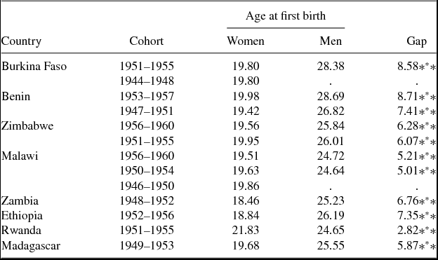
As the theory predicts, we do see large age gaps in the countries with large fertility gaps. Table 4 shows the average age at first birth by gender and the resulting age gap for all eight countries. The age gap is highest in the highly polygynous countries, namely Benin and Burkina Faso. For example, the gender age gap at first birth in Burkina Faso is 8.6 years. For the lower polygyny countries, such as Zimbabwe, Malawi, Zambia, and Ethiopia, the age gap is significantly smaller. For Rwanda, it is particularly small while it is somewhat surprisingly high for Madagascar.
Age at first birth by gender
Notes: ***1%, **5%, and *10% significance level. The means are tested on equality based on a two-sample t-test with sampling weights.
Yet, are the age gaps large enough to quantitatively explain the extremely large fertility gaps we found? We can use equation (1) to check. Consider the 1951–1955 cohort in Burkina Faso as an example. From Table 4 we know that on average women have their first birth at 19.8 and men at 28.4. Looking at population data from the 1980 census, we find that there were 225,200 25–29 year-old men at the time, and 355,000 15–19 year-old women, i.e., a ratio of 1.58 women per man.Footnote 24 Assuming ξ = 1 (i.e., no time trend in fertility), equation (1) would predict that there are 1.58 as many children per man than per women. Equivalently, given that female fertility in the data is 7.48, one would predict that male fertility should be 11.8. The predicted gap of 4.3 is even larger than the actual fertility difference we observe in the DHS of that cohort (2.76), and hits the data for the cohort of 1944–1948 almost exactly.
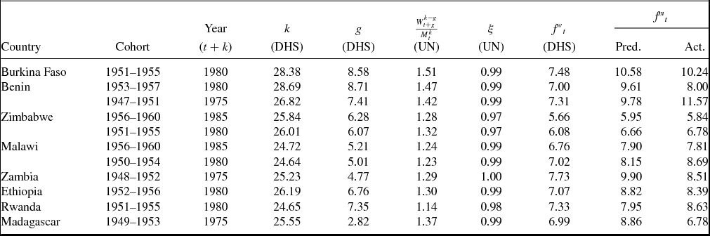
In Appendix B.2, we perform a more precise version of this calculation for all cohorts where age at first birth is available. Specifically, for each gender we compute gender sex ratios using population sizes at the appropriate ages (reported in the UN World Population Prospects, 2015) and take the time trend in female fertility rates into account. The resulting estimate for male fertility of the cohort of 1951–1955 in Burkina Faso is 10.58 and hence a fertility gap of 3.1 children, which is very close to the 2.76 observed in DHS data.
Figure 3 plots predicted male fertility against actual male fertility for all countries and cohorts where age at first birth is available. The correlation between the two is quite high (0.74). While the actual fertility difference will depend on the exact matching of partners across cohorts, which is unobservable in the DHS, Figure 3 illustrates that our observed gender gaps are close to what we would estimate with available information on age gaps and cohort sizes, and hence not likely to purely reflect measurement error in fertility reporting.
Predicted versus actual male fertility.
3.2. Alternative Explanations Based on Measurement Issues
In this section, we explore whether the large gender gaps in fertility could be an artifact of measurement. First, it is possible that differential mortality biases our estimates of average fertility. Naturally, by using retrospective fertility outcomes of men and women aged between 40 and 59, we focus on people who survive to that age. If high fertility increased mortality for women, then we could be systematically missing the high fertility women, which would downward bias the female fertility estimates. However, we find this an unlikely explanation, because if women die due to pregnancy-related reasons, they often die when pregnant with their first child.Footnote 25 This would bias results in the opposite direction and could clearly not explain why the fertility of men is higher than that of women. Furthermore, the fact that the fertility gap is very different across countries, makes differential mortality unlikely to be the main explanation, unless one considered that such differential mortality only existed in some of the countries.
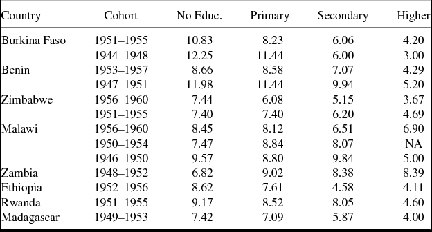
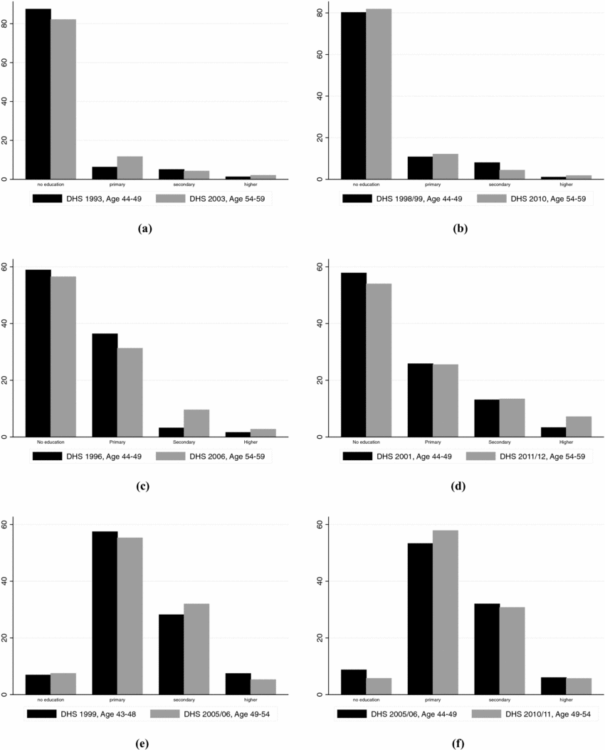
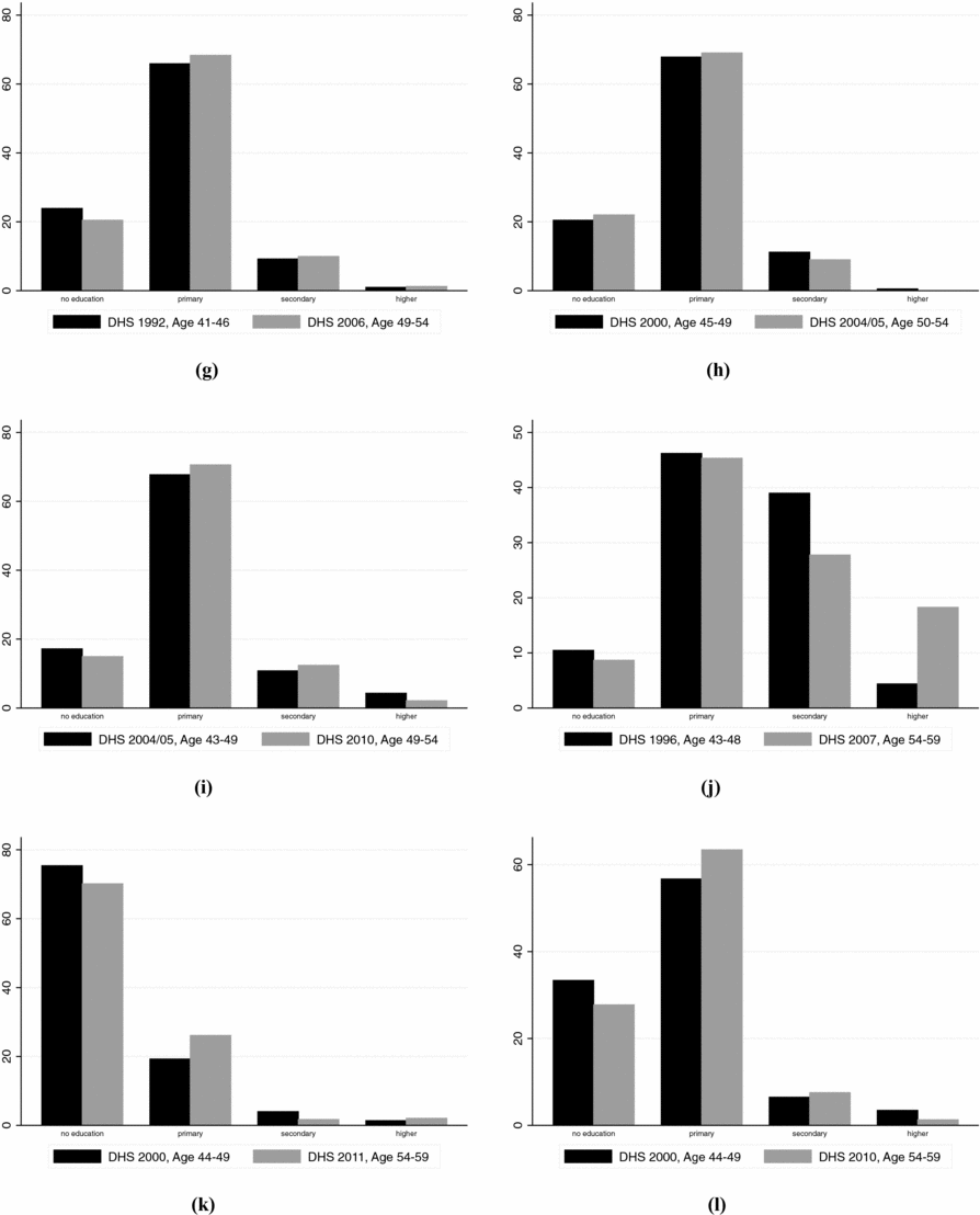
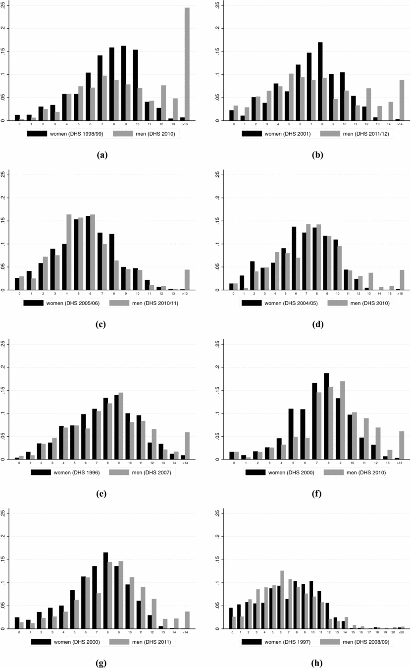
Similarly, it could be possible that richer men live longer and have more children than poorer men, which would bias our male fertility estimates upwards. To get a sense of whether selective male mortality by wealth is an issue, we compare men of the same cohort across survey rounds. Since there is no good measure of wealth in the data, we use education instead. For each country, we compare completed schooling levels among men of a particular cohort at different ages using two consecutive DHS samples to gauge whether average education is different when measured at older ages (which would surely be due to selective mortality rather than schooling investment!). Figure A1 in Appendix A depicts education histograms for each cohort we analyze. The first thing to note is that the histograms look remarkably similar when measured at different ages. Where the histograms differ, the discrepancies do suggest that more educated men live longer. This is most pronounced in Zambia, and to some extent also in Benin. However, it is also the case that male fertility is decreasing in education for all countries in our sample other than Malawi and Zambia, where it is relatively constant across education levels (Table A3). This suggests that, without selective mortality, average male completed fertility would be even higher and hence gender gaps would be even larger than those reported in the paper in six out of eight countries, and should not bias our fertility results in the remaining two.
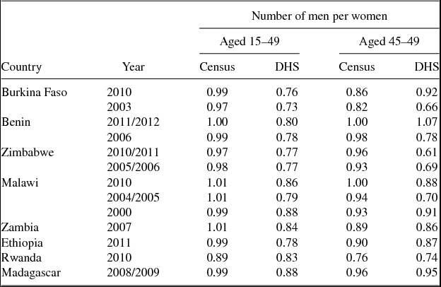
Second, it could be the case that the DHS is not representative of men and we are systematically missing those men who remain childless.Footnote 26 As one indicator, we compare the sex ratios (number of men per woman) based on national census data published by the UN with those in the DHS. If men were systematically missing in the DHS data, the sex ratios would be significantly lower than in the census data. We calculate the ratio of interviewed men and women, adjusting for the fraction of sampled households in which men are supposed to be interviewed. These sex ratios are presented in Table 5, with the left two columns presenting the ratios for the age group of 15 to 49 years and the right two columns only for those aged 45–49. Such a comparison is not possible for older cohorts (50–59), namely those of relevance for our analysis, since women are only interviewed until age 49. Even though the DHS sex ratios are systematically lower for the whole age group 15–49 in all countries (indicating that the DHS covers fewer men than would be representative) this is mainly driven by the younger cohorts. For the cohort aged 45–49, closest to the relevant group of people, the discrepancies between the sex ratios is less pronounced and even negative for the surveys in Burkina Faso in 2010 and Benin in 2011/2012. Thus, we do not believe that the large gender gaps could only be explained by missing men in our analysis.
Sex ratios
Source: The Census sex ratios are published by United Nations (2015) and based on national census data.
Third, could there be some systematic over- or under-reporting of fertility, differing for men and women? Given that women spend nine months in pregnancy and typically another year or more nursing, and since giving birth itself can be a long and painful process, it seems unlikely that a woman would not remember all her children. These arguments do not apply to men. Moreover, a man can never be absolutely sure that a child is truly his own. Thus, there could be double-counting of children if several men claimed the same child. Alternatively, there could be under-reporting of male fertility if some children were not attributed to any father. A small body of the literature exists concerning the issue of reporting bias in male fertility. There seems to be some evidence of male under-reporting of fertility (for example, Rendall et al., Reference Rendall, Clarke, Peters, Ranjit and Verropoulou1999, find that men tend to severely under-report their non-marital births in data from the US and the UK), although other papers find no difference in reporting bias between men and women (e.g., Fikree, Gray, and Shah, Reference Fikree, Gray and Shah1993, based on a small sample of men and women in Vermont). Probably more relevant for our study is evidence from other African countries. Ratcliffe et al. (Reference Ratcliffe, Hill, Harrington and Walraven2002) analyze data from the Gambia, a highly polygynous country, finding no difference in the reliability of male versus female fertility reports. Similarly, Hertrich (Reference Hertrich1998) finds no difference in the reliability of reporting live births between men and women in Mali. Given that none of the studies find that men over-report fertility, it seems highly unlikely that the gender gaps we find in fertility are an artifact of male reporting biases.
4. FERTILITY INEQUALITY HIGHER FOR MEN
Thus far, we have established that on average men have more children than women in almost all our samples. We now turn to analyzing the heterogeneity in fertility behavior separately for men and women. Heterogeneity of fertility has implications for the evolution of income inequality in a society because the correlation between fertility and income determines the resource distribution in the next generation. In general, endogenous fertility leads to an amplification of income inequality over time since the relationship between income and fertility is negative in most societies – see Jones and Tertilt (Reference Jones, Tertilt and Rupert2008). If fertility inequality is much larger for men than for women, models of income inequality should take this into account.
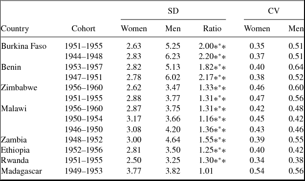
To investigate this, Table 6 displays two measures of fertility inequality for the eight countries: the standard deviation and the CV. The first thing to note is that the standard deviation of fertility of men is much higher than for women. For example, the standard deviation of the 1951–1955 cohort in Burkina Faso is 5.25 for men, compared to only 2.63 for women.
Fertility inequality by gender
Notes: SD represents the standard deviation. CV is the coefficient of variation. ***1%, **5%, and *10% significance level. All variance ratio tests (with or without weights) lead to the same conclusion that the variances are statistically different from each other at the 1% confidence level, except for Madagascar where the test with weights suggests they are different while the test without weights does not.
To better compare fertility inequality across gender and countries with very different means, the table also includes the CV. Even controlling for the fact that mean fertility is lower for women, we find a larger degree of inequality for men than women in all countries.Footnote 27 Accordingly, women are more similar to each other in their fertility behavior than men are to each other in almost every country that we consider. Again considering the example of the 1951–1955 cohort in Burkina Faso, we find a CV for men of 0.51 compared to only 0.35 for women. Interestingly, the CV for men is very similar across countries, at around 0.5.
The finding that male fertility inequality is larger than female inequality is strongest in the high polygyny countries. Figure 4 plots relative fertility inequality against the polygyny rate. The correlation is high (0.94) and the R 2 of the fitted regression line is 0.89. In Burkina Faso and Benin, the highest polygyny countries, the gender ratio of the standard deviations is about 2 – compared to a ratio of about 1.3 in most of the medium polygyny countries. In Madagascar, which is essentially monogamous, the standard deviation is almost identical for men and women. Put differently, high male heterogeneity in fertility directly translates into high female heterogeneity in monogamous countries. This is not the case in countries with a high degree of polygyny where men have another margin of adjustment. Those men who want many children do not necessarily need a woman who agrees, but rather they can have children with multiple women.
Gender gaps in fertility inequality versus male polygyny rate.
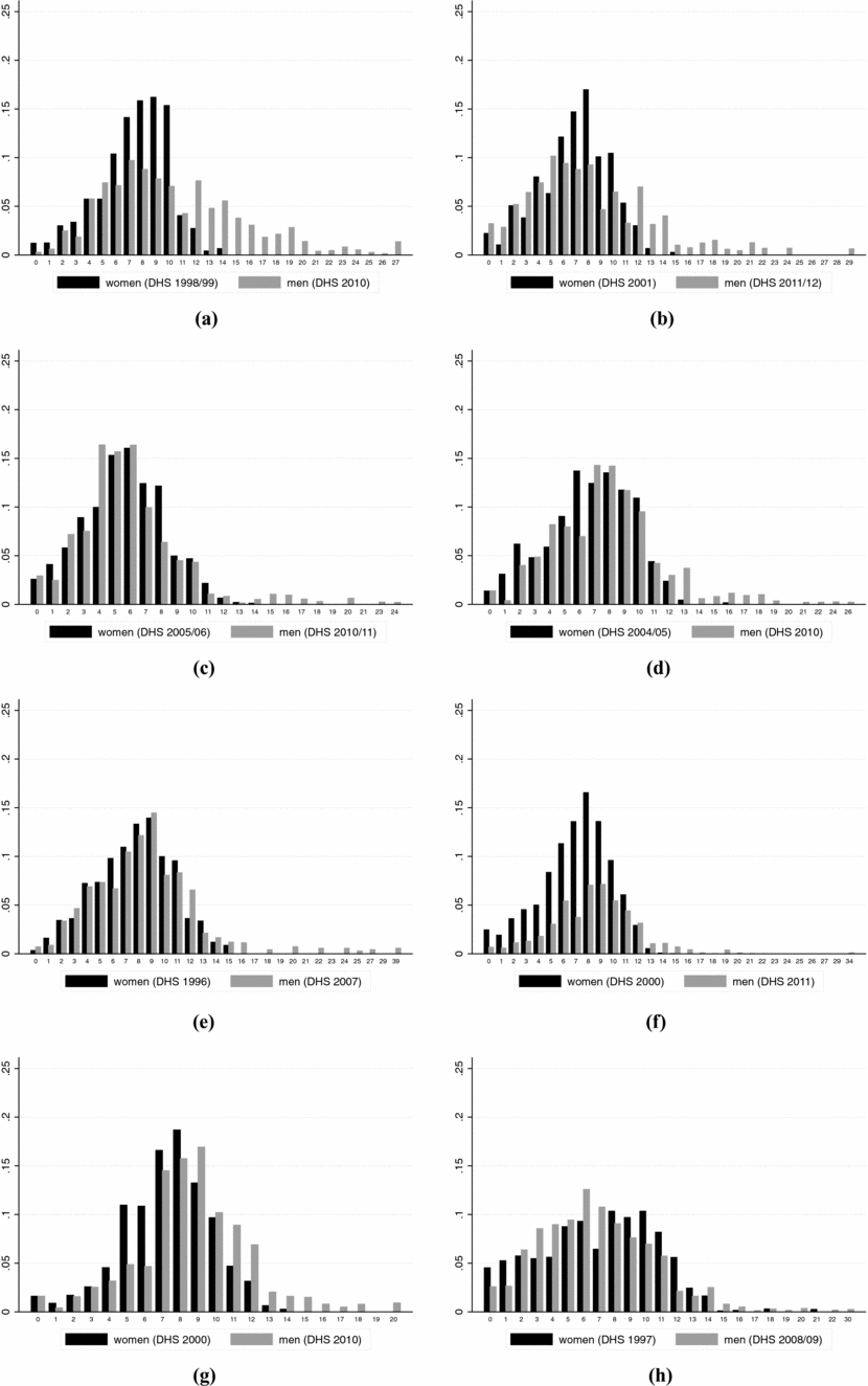
To gain a better sense of how male and female fertility behaviors differ, Figure 5 displays the distribution of fertility outcomes. For each country, we have plotted only one distribution, based on the most recent cohort for which we have data. Each panel includes separate distributions for men and women. The first thing to note is that the distribution for men is flatter than the female distribution and shifted to the right. Again, the differences between men and women are most striking for Burkina Faso and Benin. While there are no women with more than 14 (15) children in Burkina Faso (Benin), many men have higher completed fertility rates, with some having up to 29 children. The percentage of men with more children than the highest fertility of women is quite large, at 19% in Burkina Faso and 8% in Benin. Figure A2 in the Appendix shows the fertility distribution censored at the maximum female completed fertility rate. It shows that while 24% (9%) of the men in Burkina Faso (Benin) have more than 13 (14) children, only 0.7% (0.3%) of the women do.
Fertility distribution. (a) Burkina Faso (Cohort 1951–1955). (b) Benin (Cohort 1953–1957). (c) Zimbabwe (Cohort 1956–1960). (d) Malawi (Cohort 1956–1960). (e) Zambia (Cohort 1948–1952). (f) Ethiopia (Cohort 1952–1956). (g) Rwanda (Cohort 1951–1955). (h) Madagascar (Cohort 1949–1953). Note: Women and men with no children at all are also considered.
In the countries with moderate polygyny, the pattern is less pronounced, but qualitatively similar. In each case, there is a sizable fraction of men having more children than the highest fertility women, at 4% in Zimbabwe, 3% in Malawi, 5% in Zambia, 2% in Ethiopia, and 4% in Rwanda. What is also interesting is that no large fraction of childless men is observed in any of the eight countries. One might have thought that high male fertility inequality means many men with high numbers of wives and children and equally many with no wives and children, yet this is clearly not the case. On the contrary, as shown in Figure 5, for the youngest cohorts we consider the fraction of men without any children is lower than the fraction of women with no children in Burkina Faso, Madagascar and Ethiopia. In Malawi and Rwanda, the fractions are essentially the same. Only in Benin, Zimbabwe and Zambia do we have a slightly higher fraction of childless men than women, although the numbers are still small in absolute terms, with around 3% of men having no children in Benin and Zimbabwe and less than 1% in Zambia (for older cohorts, see Table 3).
Finally, turning to Madagascar, the only country with essentially no polygyny in our sample, it is striking how similar the distributions are for men and women. Less than 1% of men have more children than the highest female fertility (which admittedly is particularly high at 21 children).
5. GENDER GAPS IN DESIRED VERSUS ACTUAL FERTILITY
It is well-known that the desired fertility of men and women often does not coincide in survey data. Especially in developing countries, men tend to say that they desire more children than women (Bankole and Singh, Reference Bankole and Singh1998).Footnote 28 The typical interpretation is that women bear a higher share of the cost of child-rearing, which makes children relatively more expensive for women. For example, one cost is the risk of dying in child birth, which is obviously born by women only. But how is this discrepancy in preferences resolved? One could view the actual fertility outcome as the result of a bargaining game between husband and wife, possibly with asymmetric information. This is the approach of Doepke and Kindermann (Reference Doepke and Kindermann2013), who built a model of spousal bargaining over fertility outcomes to analyze fertility in Europe, as well as Rasul (Reference Rasul2008), who analyzes discordant fertility preferences in Malaysia. The importance of asymmetric information is emphasized in Ashraf, Field, and Lee (Reference Ashraf, Field and Lee2013), who provide evidence from a field experiment that women conceal contraceptive use from their husbands if given a chance, reducing child-bearing.
Our finding of a gender gap in realized fertility allows a novel interpretation of the gender gap in desired fertility. In particular, it shows that spouses do not need to agree on fertility outcomes. If men want more children than women, they can do so by having children with multiple women.Footnote 29 Thus, we now analyze the extent to which the gap in desired fertility is explained by the gap in actual fertility. If the two gaps coincided, then no bargaining about babies would be necessary, given that each spouse can realize their desire individually.Footnote 30
To calculate desired fertility, note that the DHS asks two questions on the issue. If a person has living children, she/he is asked: “If you could go back to the time you did not have any children and could choose exactly the number of children to have in your whole life, how many would that be?” For people without living children, the question is rephrased as: “If you could choose exactly the number of children to have in your whole life, how many would that be?” Naturally, these questions are somewhat problematic as they are asked retrospectively. For example, a person with many children might be reluctant to report having wanted fewer. However, we see no reason to believe that such ex-post rationalization should differ systematically by gender. Since, we are interested in the difference between men and women, we do not see the reporting bias as a major concern. As in our previous analysis, we report averages by birth cohorts. In other words, we are not comparing gaps within couples, but rather analyze average gaps within cohorts of men and women.
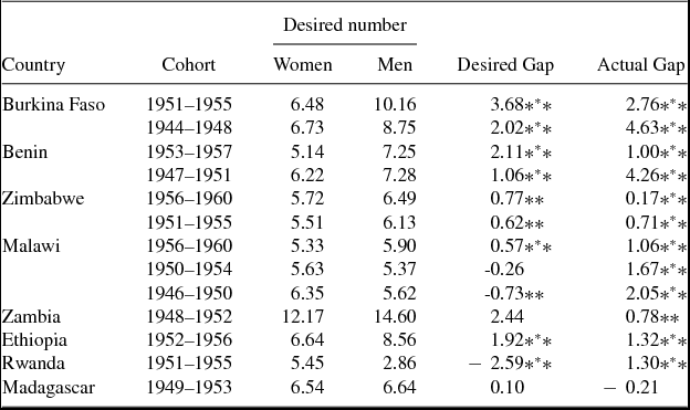
Table 7 shows the mean desired number of children for men and women for all countries and cohorts under consideration. The first thing to note is that we indeed find a large positive and significant gap in the desired number of children in eight of the cohorts that we consider. However, we also observe no significant gap or even a negative one (women wanting more children) in some countries. The positive gaps in Zambia and Madagascar are also not statistically significant. In Malawi, the results differ by cohort: for the youngest cohort, we find a significant positive (though relatively small) gap of half a child, while the gap for the older cohorts is negative or insignificant.
Desired number of children by gender
Notes: People are asked how many children they would like to have in life. Those who answer, “whatever god wants” or “don’t know” are not considered here. The significance levels are ***1%, **5%, and *10%. The means are tested on equality based on a two-sample t-test with sampling weights.
The size of the gap again seems quite systematically related to polygyny. Figure 6 plots the desired fertility gap against the polygyny rate. The correlation is fairly high (0.52) and the R 2 of the fitted regression line is 0.27. The two high polygyny countries have extremely large gaps. In Burkina Faso, men of the 1951–1955 cohort want on average 3.68 more children than women. Similarly, in Benin, men want between 1 and 2.1 more children than women, depending on the cohort considered. We see more mixed results in Malawi, Zambia, Ethiopia, and Rwanda, the countries with relatively low levels of polygyny. Here, the gap is never larger than 2.5 children, and is either negative or insignificant for several cohorts. Finally, in Madagascar, the country with almost no polygyny, we do not see men wanting more children at all. There is no significant positive gap.
Desired gender gap in fertility versus male polygyny rate.
Comparing the desired gap with the actual gap, it becomes clear that a large fraction of the desired gap is actually realized in many of the countries we consider (see Table 7). Figure 7 illustrates this visually.Footnote 31 The ratio of desired fertility (male to female) is on the horizontal axis and the actual fertility ratio on the vertical axis. We included the 45-degree line as a benchmark on which all of the desire gap would be realized. Clearly, there is a strong positive relationship between the desired ratio and the realized ratio. Thus, a large part of the disagreement in fertility seems to translate into men having children with multiple women, although not all of it.
Desired versus actual fertility ratios across countries.
6. DEMOGRAPHIC TRANSITION
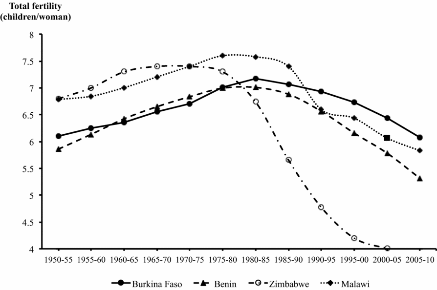
Conventional wisdom is that the demographic transition in most Sub-Saharan African countries started relatively late and its pace has been slower than in other regions (see Casterline, Reference Casterline2001; Bongaarts, Reference Bongaarts2008).Footnote 32 Such statements are usually based on TFR, i.e., measures of female fertility. Figure 8 plots TFR for Benin, Burkina Faso, Malawi, and Zimbabwe over the second half of the 20th century. With the exception of Zimbabwe, TFR did not start falling until the late-1980s, and even then, they fell relatively slowly. For example, in Burkina Faso, total fertility at its peak in the mid-1980s was about 7.2 children per woman, before falling within the next two decades to only 6.1 – a little more than a one child decline over a period of 20 years.
Demographic transition based on total fertility rates.
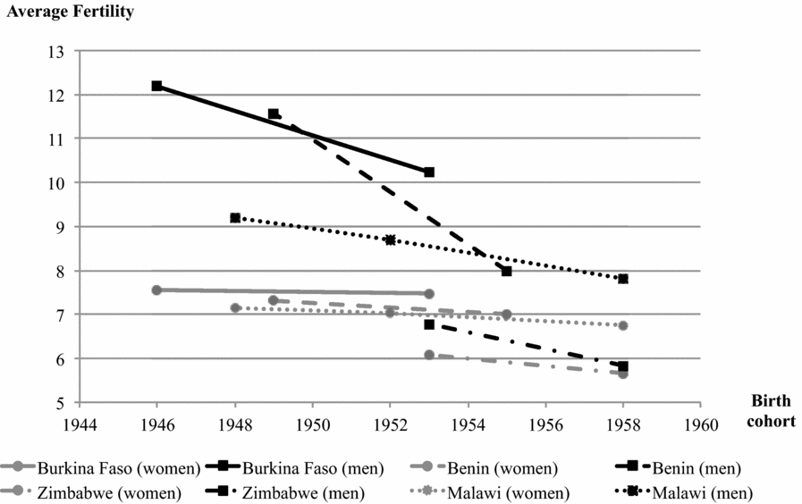
Clearly it is not only relevant when choices are made (when children are born), but also who makes those choices. Thus, one would like to know which cohorts of parents started choosing to have smaller families. Figure 9 plots children ever born by birth cohorts from the DHS data. The average numbers of children are depicted in red for women and blue for men. Naturally, given the limited number of cohorts in our data, the figure does not give a complete picture of the entire demographic transition.Footnote 33 Nonetheless, we observe a striking pattern, even for the short time span that we consider. While there is essentially no visible decline in fertility in any of the four countries for women born between 1944 and 1960, we see a sharp decline for men of the same cohorts in all countries. While men of the 1944–1948 cohort in Burkina Faso had 12.2 children on average, less than 10 years later, this had declined to 10.2. Similarly, in Benin we see an extremely sharp decline, from 11.6 to 8.0 within 6 years. Also, in Malawi, the number of children per man fell from 9.2 to 7.8 within 10 years. Finally, in Zimbabwe, where we consider relatively recent cohorts, fertility levels for both men and women are already lower than in the other countries. Still, male fertility declined from 6.8 to 5.8 in 5 years, almost reaching female fertility of 5.7 for the last cohort born between 1956 and 1960.
Demographic transition based on children ever born by gender of parent.
This analysis raises the possibility that the idea of a slow demographic transition, or even a stalling fertility decline, which has been much emphasized by demographers, could be an artifact of focusing exclusively on female fertility. With regard to men, Figure 9 suggests, fertility has been falling quite sharply. We do believe that documenting the differential speed of the demographic transition by gender is quite important. Lower fertility typically goes hand-in-hand with higher child quality (greater investments into or higher bequests to each child). If this quantity–quality trade-off is at work, and if men have more resources than women, then the fact that fertility is falling steeply for men should be more relevant than that it is stalling for women. Of course, we show only a 10-year window for each country, i.e., only a short snapshot of the demographic transition. It remains to be seen how robust this differential speed is when considering longer time series and more countries.
7. CONCLUSION
We use novel data provided by the DHS male questionnaires to analyze differences in completed fertility by gender in Sub-Saharan Africa. For Benin, Burkina Faso, Zimbabwe, Zambia, Malawi, Ethiopia, and Rwanda, we observe on average higher completed fertility for men than for women of the same birth cohorts. The empirical analysis shows that this discrepancy is largest in highly polygynous countries. We document that an important factor for the large gender gaps is that men have children beyond their mid-40s (the onset of menopause for the majority of women). We show that in countries with growing population and large age gaps, male fertility is necessarily higher than female fertility. Such a situation typically coincides with men having multiple wives, although this is not strictly necessary.
Second, for highly polygynous countries, we document a notably higher inequality in male fertility than in female fertility, measured through the standard deviation of fertility. This is less pronounced in countries with low or almost no polygyny. This means that for (almost) monogamous countries, heterogeneity in male fertility translates one-to-one into female heterogeneity, while men in highly polygynous countries have an additional margin of adjustment breaking the link between male and female heterogeneity.
Third, the difference in average fertility provides a novel interpretation for the gender gap in desired fertility. Existing interpretations are based on the assumption that realized fertility does not differ between spouses. We show that average realized fertility between men and women of the same cohort can differ, and that there is a positive relationship between the average desired and realized fertility gaps. In line with the literature, we find that men want more children than women in most of the countries. However, a disagreement in these desires can be resolved by men having children with more than one woman.
Finally, we find that the size and speed of the demographic transition depends on the gender considered. In Burkina Faso, Benin, Malawi, and Zimbabwe the size and speed of the fertility decline have been much more pronounced for men than for women of the same cohort.
We believe that these results may be important for researchers building theories of fertility behavior. This paper shows that the facts may look somewhat different depending on whether they are derived from men or women. Inequality in fertility is a strong example. Our results show that heterogeneity in fertility outcomes is much larger for men than for women. How does this affect the resource distribution in the next generation? Historically, the relationship between income and fertility is negative in most societies. Thus, endogenous fertility leads to an amplification of income inequality over time. Taking the distribution of children across men into account, this amplification could be even more severe than estimates based on women would suggest. However, if it is the rich men who have the most children in those societies where men have children with multiple women, then this would mitigate the endogenous inequality propagation across generations.
In this paper, we have analyzed fertility gaps across gender in eight Sub-Saharan African countries. Conducting a similar analysis for other countries would be very interesting and is left for future research. Finally, while we speculate that polygyny is the most important factor in explaining gender gaps in fertility, we have not formally investigated this hypothesis. Other possibilities are non-marital child-bearing, divorce followed by remarriage, death with subsequent remarriage, or simply large fractions of women remaining childless. Decomposing the observed gender fertility gaps according to these various possibilities would be an interesting avenue to pursue, although data constraints will not make this an easy task.
A. DATA APPENDIX
A.1. Robustness on Completed Fertility
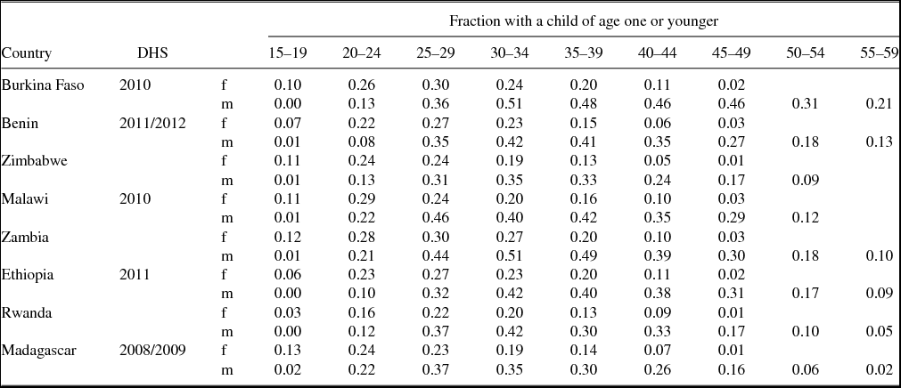
We can also use the data to check how reasonable our assumption of completed fertility is at ages (depending on the country/cohort) 50–54 for men and 42–45 for women. The survey includes a question on the age of the youngest child. We calculate the fraction of men and women of various ages who have a child below one, based on the most recent DHS for each country. The numbers are given in Table A1, which shows a hump-shaped pattern in all countries and for both sexes. The peak fertility occurs for women between the ages of 20 and 29 in all countries, before falling rapidly after age 34. For example, while a quarter to a third of all 25–34 year-olds have a child that was born in the last year, this declines to 11% or less by 40–44. Very few women aged 45 or older have infants in the household. The highest percentage is in Benin, Malawi, and Zambia, with 3% of 45–49 year-old women having a child born during the previous year. Therefore, we think that it is fairly innocuous to use completed fertility rates of women aged 41 and older as a proxy for completed lifetime fertility rates.
Indicator for completed fertility
Sample implementation
Male completed fertility by education
The corresponding figures for men look somewhat different, particularly in highly polygynous Burkina Faso. For men, peak fertility occurs at later ages, between 25 and 34 in all countries, but remains very high until age 49. In some countries, there is still a large fraction of men in the oldest age group who have a child aged one or younger, as high as 21% for 55–59 year-old men in Burkina Faso. Therefore, it is difficult to argue that men have truly completed their fertility by this age. However, this finding biases our results concerning the average fertility of men downwards. In other words, adjusting for children that men have at even older ages would further increase the male fertility rates and thereby increase the gender gaps in fertility reported in Table 3. Note also that for countries with low levels of polygyny, the fraction of men with a child born in the previous year peaks at an earlier age and is considerably lower for the older ages and thus even less problematic for our assumption that fertility is completed for men in their mid-50s.
A.2. Additional Tables and Figures
Male distribution of education. (a) Burkina Faso, Cohort 1944–1948. (b) Burkina Faso, Cohort 1951–1955. (c) Benin, Cohort 1947–1951. (d) Benin, Cohort 1953—1957. (e) Zimbabwe, Cohort 1951–1955. (f) Zimbabwe, Cohort 1956–1960. (g) Malawi, Cohort 1946–1950. (h) Malawi, Cohort 1950–1954. (i) Malawi, Cohort 1956–1960. (j) Zambia, Cohort 1948–1952. (k) Ethiopia, Cohort 1944–1948. (l) Rwanda, Cohort 1951–1955.
Fertility distribution (censored). (a) Burkina Faso (Cohort 1951–1955). (b) Benin (Cohort 1953–1957). (c) Zimbabwe (Cohort 1956–1960). (d) Malawi (Cohort 1956–1960). (e) Zambia (Cohort 1948–1952). (f) Rwanda (Cohort 1951–1955). (g) Ethiopia (Cohort 1952–1956). (h) Madagascar (Cohort 1949–1953).
B. FERTILITY AND MARRIAGE MARKET ACCOUNTING
B.1. Theory
This appendix demonstrates how male and female fertility can differ even though each child has a father and a mother. It illustrates that male and female fertility need not coincide, not even on average. We also show that polygyny is likely an important factor (even though it is theoretically not necessary). The notation is closely related to Neelakantan and Tertilt (Reference Neelakantan and Tertilt2008).
Let fmt be the completed fertility rate of men of cohort t and fwt the completed fertility rate of women in cohort t. Let Mkt be the size of the male cohort born in t at age k, i.e., in year t + k. Similarly, Wkt denotes the number of women of cohort t at age k. Now, assume that men have children when they are k years old. Then, the total number of children born in year t + k to all men is fmtMkt. Further, assume that men have children with women who are g years younger. Then, the number of children born to all women in year t + k is fw t + gW k − gt + g.
Clearly, the aggregate number of children born to all women in year t + k and the number of all children fathered in the same year must coincide. Thus, we get the following fertility “market clearing” condition:Footnote 34
 $$\begin{equation}
f^m_t M^k_t = f^w_{t+g} W^{k-g}_{t+g} .
\end{equation}$$
Note that our data compares fertility of the same birth cohorts of men and women, not, as the expression above, children born in the same year. Thus, our data gives fmt and fwt. Define  $\xi = \frac{f^w_{t+1}}{f^w_t}$ as the change in (completed) female fertility from one cohort to the next. Then, male fertility of cohort t can be written as
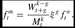 $$\begin{equation}
f^m_t= \frac{W^{k-g}_{t+g}}{M^k_t} \xi ^{g}f^w_{t}.
\end{equation}$$
The equation tells us that if there is more than one women per man at childbearing age ( $\frac{W^{k-g}_{t+g}}{M^k_t}>1$) and female fertility is stable across cohorts, ξ = 1, male fertility will be higher than female fertility, fmt > fwt.
Even though the sex ratio at birth is typically close to one, the sex ratio at childbearing age ( $\frac{W^{k-g}_{t+g}}{M^k_t}$) may be greater than one for at least three reasons. First, population growth in conjunction with age gaps in childbearing, g > 0, implies that we are comparing different cohorts of women and men–women coming from a larger cohort. Second, even if the population was not growing, mortality may differ by gender. If male mortality is higher, e.g., due to wars, then the relevant sex ratio will be greater than one. Third, even if mortality rates do not differ by gender and the population is constant, the sex ratio at childbearing age will still be greater than one as long as men have children with younger women and there is some (gender-neutral) mortality.
In addition, ξ would typically be smaller than one for most countries. Thus, fertility decline adds another reason for male and female fertility of the same cohort to differ: the faster (female) fertility is decreasing across cohorts, the smaller the gender gap in fertility – assuming men have children with younger women. The size of the age gap matters here as well as it multiplies the effect of declining fertility. Note that this last point alone (i.e., declining fertility over time coupled with positive age gaps) would lead to a gender fertility gap below one, i.e., men would have fewer children than women.
One might wonder if different marriage cohort sizes necessarily imply polygyny. This is actually not the case. So far we have only considered aggregate demand and supply for children in a given year, i.e., market clearing for fertility. What about market clearing for marriage? Following the notation in Neelakantan and Tertilt (Reference Neelakantan and Tertilt2008), let nt be the average number of wives per man of cohort t. Further, let smt and swt be the fraction of males and females of cohort t that remain single. Note that we are equating being single here with not having children. Similarly, we use the word “wife” for all women a man has children with. Then, the total number of brides that are being demanded by men of cohort t is
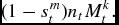 $$\begin{equation*}
(1-s^m_t) n_t M_t^k.
\end{equation*}$$
Again, assuming these men marry women g years younger than them, and assuming polyandry (i.e., women marrying multiple men) does not existFootnote 35, the total number of brides offered by women in year t + k is (1 − sw t + g)W k − gt + g. Marriage market clearing says that the demand and supply for brides needs to be equal, which can be written as:
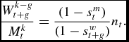 $$\begin{equation}
\frac{ W_{t+g}^{k-g}}{ M_t^k} = \frac{(1-s^m_t)}{ (1-s^w_{t+g})} n_t.
\end{equation}$$
This expression shows that if there are more women than men having children in year t + k (which is needed for a positive fertility gap, as explained above), then either the average man is fathering children with more than one wife (nt > 1) or more women remain childless than men (sw t + g > smt).
B.2. Empirics
The goal of this appendix is to use additional data together with the theory in the previous section to investigate whether the gender fertility gaps we measured in our eight countries are reasonable, i.e., not an artifact of measurement. As equation (3) above showed, gender gaps in fertility are directly related to relative marriage cohort sizes. As the theory showed, the age gap plays an important role. Now, we use data together with equation (3) to verify this.
For each cohort, we first find proxies for k, g, Mkt, W k − gt + g and ξ either from our own calculations based on the DHS or from the United Nations (2015). We then use female completed fertility rates from Table 3 together with equation (3) to predict male fertility. Next, we compare the predicted male completed fertility rate to the actual male completed fertility rate in Table 3.
Specifically, we predict male fertility for each of the 11 cohorts in Table 3 for which age at first birth is available (see Table 4). For each cohort, we need data on male and female ages at first birth (k and g) and the sizes of the relevant male and female cohorts (W k − gt + g, Mkt). We also need a long-run trend in (female) fertility as a proxy for ξ. We now describe in detail what data we use for each of these items. The data is reported in Table A4 and A5.
• Average age at first birth for men (k) is calculated directly from DHS (see Table 4). Since this information is not available for Burkina Faso 1944–1948 and Malawi 1946–1950, we drop these two cohorts.
• The age gap between men and women (g) is simply the difference in the ages at first birth for men and women. This gap is also taken directly from Table 4.
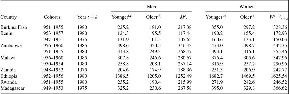
• Mkt and W k − gt + g: These are simply the absolute number of people of a specific cohort at a specific age (namely at marriage). In principle, these could be directly taken from the data. In practice, we use data from United Nations (2015) which provides population sizes by year and age in 5-year age brackets, which for this particular calculation are too coarse categories. Take Rwanda as an example. Our 1951–1955 male birth cohort marries on average at age 24.65 (see Table 4). Thus, ideally we need to know how many males of age 24.65 were around in 1976–1980, which is not available. Instead, we have population numbers for age categories 20–24, 25–29, 30–35, etc. in 1980. In the Rwanda example, in 1980 there were 235,200 men in the 20–24 age category and only 190,400 in the 25–29 age category. Since 24.65 is in the middle of the two brackets and since the population sizes are very different from each other, simply using one of those numbers will not be a good proxy. Instead, we take a weighted average where the weights are such that the average age is exactly 24.65. In this specific example, since on average men in the 20–24 category are 22.5 years old and those in the 25–29 category are 27.5 years old, the weights are 0.57 and 0.43 respectively (since 0.57 × 22.5 + 0.43 × 27.5 = 24.46). Using these weights, we calculate that the relevant male marriage cohort size is 215,990. Redoing the same for women in Rwanda, we find a relevant female marriage cohort size of 246,520.
We use the same procedure to construct the sizes of the relevant marriage cohorts of men and women for all countries/cohorts we analyze. The details are summarized in Table A5. Note that the birth cohort year reported in the table is the male year, while the female cohort is born g years later. The columns labeled “younger” and “older” (both for men and women) always give the raw numbers from the United Nations (2015) for the two age categories closest to the age we actually need, while the columns Mkt and W k − gt + g give the weighted average we constructed as described above. Table A4 reports the ratio
 $\frac{W^{k-g}_{t+g}}{M^k_t}$.
• Change in female fertility across cohorts one year apart, i.e, ξ. From the United Nations (2015), we get age-specific fertility rates for 5 year age-groups and 5 year periods from 1950–2015. First, we calculate the cohort fertility rate for the 1950–1955 birth cohort by adding up the fertility rates for age 15–19 from 1970–1975, age 20–24 from 1975–1980, age 25–29 from 1980–1985, age 30–34 from 1985–1990, age 35–39 from 1990–1995, age 40–44 from 1995–2000 and age 45–49 from 2000–2005. Second, we calculate the cohort fertility rate of the 1960–1965 cohort by adding up age-specific fertility rates from 1980 to 2015. Since these cohorts are 10 years apart, the ratio between these two fertility rates is then equal to ξ10 from which we can infer ξ. Column 7 in Table A4 reports the results for each country.
• Column 8 simply repeats female completed fertility from our main Table 3.

Predicted versus actual male fertility
Population size at childbearing age
Equipped with all these ingredients, we now use equation (3) to predict male fertility. The last two columns in Table A4 show the predicted and the actual male fertility side by side – they look remarkably similar. Figure 3 illustrates this finding graphically. The coefficient of correlation between predicted and actual male fertility is 0.74. These results give confidence to the main result of our paper – namely that male and female fertility in Sub-Saharan Africa are often quite different and not an artifact of measurement problems.