1. Introduction
This paper considers two types of M/G/1 queues with impatient customers. In the first model, each customer has her own waiting-time deadline; if her waiting time reaches the deadline then she leaves the system immediately. In this model, once a customer starts to receive her service she does not leave the system until the end of the service. In the second model, on the other hand, each customer has her own sojourn-time deadline, where customers in service also renege when their deadlines expire. For each model we assume that customers arrive according to a Poisson process, and their service times are independent and identically distributed (i.i.d.). We also assume that the lengths of deadlines (called patience times hereafter) are i.i.d. We denote the first model (resp. the second model) by M/G/1+Gw (resp. M/G/1+Gs) as introduced in [Reference Boxma, Perry and Stadje3]. We use the notation M/G/1+G to collectively denote the M/G/1+Gw and M/G/1+Gs queues.
We consider M/G/1+Gw and M/G/1+Gs queues that are characterized by the same arrival rate λ (λ > 0), the same service time distribution, and the same patience time distribution. Let H (resp. G) denote a generic random variable for service times (resp. patience times). For simplicity, we assume P(H = 0) = P(G = 0) = 0.
Throughout this paper we use the following conventions: For any non-negative random variable Y, Y(x): = P(Y ≤ x) denotes the cumulative distribution function (CDF),  $\overline Y (x): = 1 - Y(x)$ denotes the complementary CDF, and y(x) denotes the probability density function (p.d.f.) provided it exists. In addition, we denote quantities in the M/G/1+Gw (resp. M/G/1+Gs) queue with a superscript ‘w’ (resp. ‘s’).
We assume that patient customers may exist, who do not leave the system until the end of the service. Such customers are regarded to have infinite patience times, so that the CDF of patience times may be defective, i.e.  $\mathop {\lim }\nolimits_{x \to \infty } \overline G (x) = {g_\infty }$, where g ∞ ∈ [0, 1) denotes the probability that a randomly chosen customer is patient. On the other hand, we assume that the service time distribution has finite mean E[H]. We define ρ: = λE[H] as the traffic intensity, and we assume that ρg ∞ < 1, which ensures the stability of the M/G/1+Gw and M/G/1+Gs queues. Note that this stability condition can readily be obtained from [Reference Browne and Sigman6, Theorem 2.1].
For the M/G/1+Gw and M/G/1+Gs queues, various analytical results can be found in the literature [Reference Baccelli, Boyer and Hebuterne1, Reference Boxma, Perry and Stadje3, Reference Brandt and BRANDT4, Reference Daley8, Reference Inoue and Takine9, Reference Inoue and Takine10, Reference Kovalenko11, Reference Perry and Asmussen13]. In particular, it is shown in [Reference Kovalenko11] that the virtual waiting time distribution in each of the M/G/1+Gw and M/G/1+Gs queues is determined by a Volterra integral equation of the second kind, and the loss probability P loss is given in terms of it. Let V denote a generic random variable for the stationary virtual waiting time. With the level-crossing argument [Reference Brill and Posner5, Reference Cohen7], we have
 $${v^{\rm{w}}}(x) = \lambda \pi _0^{\rm{w}}\overline H (x) + \lambda \int_0^x {v^{\rm{w}}}(y)\overline G (y)\overline H (x - y) {\rm{d}}y,\quad x \gt 0,$$
 $${v^{\rm{s}}}(x) = \lambda \pi _0^{\rm{s}}\overline H (x)\overline G (x) + \lambda \int_0^x {v^{\rm{s}}}(y)\overline H (x - y)\overline G (x) {\rm{d}}y,\quad x \gt 0,$$
where π 0 denotes the probability that the system is empty, and it satisfies
 $$\pi _0^{\rm{w}} + \int_0^\infty {v^{\rm{w}}}(x) {\rm{d}}x = 1,\quad \quad \pi _0^{\rm{s}} + \int_0^\infty {v^{\rm{s}}}(x) {\rm{d}}x = 1.$$
Equations (1) and (2) are Volterra integral equations of the second kind, which along with the normalization conditions (3) uniquely determine the virtual waiting time distributions [Reference Pipkin14, Section 5.2].
Because Poisson arrivals see time averages (PASTA), the loss probability P loss in each model is then given by
 $$P_{{\rm{loss}}}^{\rm{w}} = {\rm{P}}(G \le {V^{\rm{w}}}) = \int_0^\infty {v^{\rm{w}}}(x)G(x) {\rm{d}}x,$$
 $$\matrix{
{P_{{\rm{loss}}}^{\rm{s}}} \hfill & = \hfill & {{\rm{P}}(G \le {V^{\rm{s}}} + H)} \hfill \cr
{} \hfill & = \hfill & {\int_{x = 0}^\infty {\rm{d}}G(x)\left(\pi _0^{\rm{s}}\overline H (x) + \int_{y = 0}^x {v^{\rm{s}}}(y)\overline H (x - y) {\rm{d}}y + \int_{y = x}^\infty {v^{\rm{s}}}(y) {\rm{d}}y\right).} \hfill \cr
} $$
Using (1), we can rewrite (4) as
 $$P_{{\rm{loss}}}^{\rm{w}} = 1 - {{1 - \pi _0^{\rm{w}}} \over \rho }.$$
The loss probability in the M/G/1+Gw queue is thus given in terms of  $\pi _0^{\rm{w}}$, whereas it seems difficult to obtain such a simple formula for the M/G/1+Gs queue.
The purpose of this paper is to derive comparison results between the M/G/1+Gw and M/G/1+Gs queues. Most previous works have focused on analysis of each model or a general impatience mechanism [Reference Brandt and BRANDT4, Reference Daley8, Reference Kovalenko11] including both of them as special cases, and only a few papers have dealt with a comparison between them. A key reference is [Reference Van Velthoven, Van Houdt and Blondia19], where  $P_{{\rm{loss}}}^{\rm{w}} \le P_{{\rm{loss}}}^{\rm{s}}$ is proved for a general discrete-time queue with geometric service times. The proof is based on the facts that
 $\pi _0^{\rm{w}} \le \pi _0^{\rm{s}}$ can be proved with a sample-path argument, and that
 $P_{{\rm{loss}}}^{\rm{s}}$ is expressed in terms of
 $\pi _0^{\rm{s}}$ (cf. (6)) if service times follow a geometric distribution [Reference Van Velthoven, Van Houdt and Blondia18]. Because the assumption of geometric service times is essential in this approach, it is not straightforward to extend this result for other service time distributions. Note that the inequality
 $P_{{\rm{loss}}}^{\rm{w}} \le P_{{\rm{loss}}}^{\rm{s}}$ is not trivial because it does not hold in general [Reference Van Houdt, Lenin and Blondia17].
Comparison between the M/G/1+Gw and M/G/1+Gs queues with the same parameters λ, H(x), and G(x) arises in the following situation, for instance. Suppose that each impatient customer is unaware of her service initiation, and she receives a notification from the server only when her service is completed. In this case, impatience refers to the sojourn time (M/G/1+Gs queue). On the other hand, if the server notifies customers of their service initiation, and if customers do not renege once their services start, then the system is represented as an M/G/1+Gw queue. Therefore, we can evaluate the effect of the notification of service initiation on the system performance by means of a comparison between the M/G/1+Gw and M/G/1+Gs queues with the same parameters λ, H(x), and G(x).
We first show that the stationary distributions of the virtual waiting time, the actual waiting time, and the sojourn time in the M/G/1+Gs queue are given in terms of those in the corresponding M/G/1+Gw queue. With this result, we then derive comparison results between the M/G/1+Gw and M/G/1+Gs queues. In particular, we provide a sufficient condition for  $P_{{\rm{loss}}}^{\rm{w}} \le P_{{\rm{loss}}}^{\rm{s}}$. Finally, we show that
 $P_{{\rm{loss}}}^{\rm{w}}$ and
 $P_{{\rm{loss}}}^{\rm{s}}$ are directly related by simple equations in two special cases: exponential service times (M/M/1+G) and exponential patience times (M/G/1+M).
The rest of the paper is organized as follows. We first consider the M/G/1+Gw and M/G/1+Gs queues in Section 2. We then consider their special cases in Section 3. Finally, we conclude the paper in Section 4.
2. Relations between M/G/1+Gw and M/G/1+Gs queues
Throughout the paper, a random variable Y conditioned on an event 𝒜 is denoted by [Y | 𝒜]. Let W denote a generic random variable for the actual waiting times of customers who receive their (partial or full) services. Also, let D denote a generic random variable for the sojourn times of customers who receive their full services. Owing to PASTA, the virtual waiting time seen by a randomly chosen arriving customer has the same distribution as V. Therefore, the waiting times W w and W s are equal to the following conditional random variables:
 $${W^{\rm{w}}}{ = _{{\rm{st}}}}\,[{V^{\rm{w}}}|{V^{\rm{w}}} \lt G],$$
 $${W^{\rm{s}}}{ = _{{\rm{st}}}}\,[{V^{\rm{s}}}|{V^{\rm{s}}} \lt G],$$
where =st denotes the equality in distribution. Similarly, we have
 $${D^{\rm{s}}}{ = _{{\rm{st}}}}[{V^{\rm{s}}} + H\,|\,{V^{\rm{s}}} + H \lt G].$$
In addition, we obtain D w from its definition:
 $${D^{\rm{w}}}{ = _{{\rm{st}}}}\,{W^{\rm{w}}} + H.$$
Lemma 1. In the stationary M/G/1+G w and M/G/1+G s queues with the same arrival rate λ , the same service time distribution H(x) (x ≥ 0), and the same patience time distribution G(x) (x ≥ 0),
 $${V^{\rm{s}}}{ = _{{\rm{st}}}}{W^{\rm{w}}}.$$
Proof. With (4) and (7), the distribution of W w is characterized as
 $${\rm{P}}({W^{\rm{w}}} = 0) = {{\pi _0^{\rm{w}}} \over {1 - P_{{\rm{loss}}}^{\rm{w}}}},\quad \quad {w^{\rm{w}}}(x) = {{{v^{\rm{w}}}(x)\overline G (x)} \over {1 - P_{{\rm{loss}}}^{\rm{w}}}},\quad x \gt 0.$$
We can then verify from (1) that P(W w = 0) and w w(x) satisfy
 $${w^{\rm{w}}}(x) = (\lambda {\rm{P}}({W^{\rm{w}}} = 0)\overline H (x) + \lambda \int_0^x {w^{\rm{w}}}(y)\overline H (x - y) {\rm{d}}y)\overline G (x),\quad x \gt 0.$$
This equation is identical to the integral equation (2), which in combination with the normalization condition (3) uniquely determines the distribution of V s. We thus conclude that V s = st W w, noting that W w is also uniquely determined by this integral equation and the normalization condition  ${\rm{P}}({W^{\rm{w}}} = 0) + \int_0^\infty {w^{\rm{w}}}(x) {\rm{d}}x = 1$.
Remark 1. The relation (11) can also be interpreted as follows. Let (U t)t ≥0 denote a stationary storage process with level-dependent release rate  $1/\overline G (x)$, and compound Poisson input with intensity λ and jump size distribution H(x). We define U as a generic random variable for the stationary distribution of (Ut)t ≥0. As shown in [Reference Perry and Asmussen13, Theorem 2.2], we have for the M/G/1+Gs queue,
 $${V^{\rm{s}}}{ = _{{\rm{st}}}}\,U.$$
This relation follows from the fact that U satisfies the level-crossing equation [Reference Bekker, Borst and Boxma2]
 $${{u(x)} \over {\overline G (x)}} = \lambda {\rm{P}}(U = 0)\overline H (x) + \lambda \int_0^x u(y)\overline H (x - y) {\rm{d}}y,$$
which is identical to (2).
On the other hand, we can relate the virtual waiting time process  ${(V_t^{\rm{w}})_{t \ge 0}}$ in the M/G/1+Gw queue to the storage process (Ut)t ≥0 by [Reference Perry and Asmussen13, p. 112]
 $${U_t} = V_{\tau (t)}^{\rm{w}},\quad t \ge 0,$$
where τ(t) (t ≥ 0) denotes a time-transformation function defined as
 $$\tau (t) = {\hat \tau ^{ - 1}}(t),\quad \quad \hat \tau (t) = \int_0^t \overline G (V_y^{\rm{w}}) {\rm{d}}y.$$
Intuitively, τ(t) represents a clock which runs 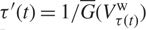 $\tau '(t) = 1/\overline G (V_{\tau (t)}^{\rm{w}})$ times faster than the original clock at time t. Because upward jumps in
 ${(V_t^{\rm{w}})_{t \ge 0}}$ occur according to a Poisson process with level-dependent intensity
 $\lambda \overline G (V_t^{\rm{w}})$, occurrences of upward jumps in
 ${(V_{\tau (t)}^{\rm{w}})_{t \ge 0}}$ follow a homogeneous Poisson process with rate λ (see also [Reference Perry and Asmussen13, p. 112]). We can then verify (14) from the fact that
 ${(V_{\tau (t)}^{\rm{w}})_{t \ge 0}}$ decreases at rate
 $1/\overline G (x)$ when
 $V_{\tau (t)}^{\rm{w}} = x$. Note that W w represents the virtual waiting time
 ${(V_t^{\rm{w}})_{t \ge 0}}$ observed just before an upward jump, which is also equal to
 ${(V_{\tau (t)}^{\rm{w}})_{t \ge 0}}$ observed just before an upward jump. Because PASTA holds for
 ${(V_{\tau (t)}^{\rm{w}})_{t \ge 0}}$, we then obtain from (14) that
 $${W^{\rm{w}}}{ = _{{\rm{st}}}}\,U.$$
Theorem 1. In the stationary M/G/1+G w and M/G/1+G s queues with the same arrival rate λ, the same service time distribution H(x) (x ≥ 0), and the same patience time distribution G(x) (x ≥ 0),
 $${V^{\rm{s}}}{ = _{{\rm{st}}}}\,[{V^{\rm{w}}}\,|\,{V^{\rm{w}}} \lt G],\quad {W^{\rm{s}}}{ = _{{\rm{st}}}}\,[{W^{\rm{w}}}\,|\,{W^{\rm{w}}} \lt G],\quad {D^{\rm{s}}}{ = _{{\rm{st}}}}\,[{D^{\rm{w}}}\,|\,{D^{\rm{w}}} \lt G].$$
Proof. Equation (16) immediately follows from (7), (8), (9), (10), and (11).
Remark 2. Let  ${D'^{\rm{s}}}$ denote a generic random variable for the sojourn time of a randomly chosen (accepted or lost) customer in the M/G/1+Gs queue. By definition, we have
 ${D'^{\rm{s}}}{ = _{{\rm{st}}}}\,\min ({V^{\rm{s}}} + H,G)$. We then obtain, from (10) and (11),
 $${D'^{\rm{s}}}{ = _{{\rm{st}}}}\,\min ({D^{\rm{w}}},G).$$
Theorem 1 shows that the stationary distributions of the virtual waiting time, the actual waiting time, and the sojourn time in the M/G/1+Gs queue are given by the conditional distributions of those in the corresponding M/G/1+Gw queue. A direct consequence of this result are the following stochastic ordering relations.
Definition 1. [Reference Shaked and Shanthikumar15, Equation (1.A.1)] Consider two non-negative random variables X and Y. X is said to be smaller than Y in the usual stochastic order (denoted by X ≤st Y) if and only if P(X > x) ≤ P(Y > x) for all x ≥ 0.
Remark 3. X ≤st Y holds if and only if E[ϕ(X)] ≤ E[ϕ(Y)] holds for all non-decreasing functions ϕ(x), provided the expectations exist [Reference Shaked and Shanthikumar15, (1.A.7)]. In particular, we have X ≤st Y ⇒ E[X] ≤ E[Y].
Corollary 1. In the stationary M/G/1+G w and M/G/1+G s queues with the same arrival rate λ, the same service time distribution H(x) (x ≥ 0), and the same patience time distribution G(x) (x ≥ 0),
 $${V^{\rm{s}}}\,{ \le _{{\rm{st}}}}\,{V^{\rm{w}}},\quad \quad {W^{\rm{s}}}\,{ \le _{{\rm{st}}}}\,{W^{\rm{w}}},\quad \quad {D^{\rm{s}}}\,{ \le _{{\rm{st}}}}\,{D^{\rm{w}}}.$$
Proof. It suffices to show that [X | X ≤ Z] ≤st X holds for any two independent non-negative random variables X and Z satisfying P(X ≤ Z) > 0; this immediately follows from [Reference Shaked and Shanthikumar15, Theorem 1.C.1] and [Reference Shaked and Shanthikumar15, Example 1.C.60].
Roughly speaking, Corollary 1 indicates that given the same parameters λ, H(x)(x ≥ 0), and G(x)(x ≥ 0), the M/G/1+Gs queue is less congested than the M/G/1+Gw queue. In particular, we can readily verify from  ${V^{\rm{s}}}{ \le _{{\rm{st}}}}{V^{\rm{w}}}$ that
 $\pi _0^{\rm{s}} \ge \pi _0^{\rm{w}}$ holds. One might expect this to imply that losses are more frequent in the M/G/1+Gs queue, i.e.
 $P_{{\rm{loss}}}^{\rm{w}} \le P_{{\rm{loss}}}^{\rm{s}}$ holds. However, this is not always the case, as we will see in Section 3. Below we derive a sufficient condition for
 $P_{{\rm{loss}}}^{\rm{w}} \le P_{{\rm{loss}}}^{\rm{s}}$.
Lemma 2. Consider the stationary M/G/1+G w and M/G/1+G s queues with the same arrival rate λ, the same service time distribution H(x) (x ≥ 0), and the same patience time distribution G(x) (x ≥ 0). The loss probabilities in these models are given by
 $$P_{{\rm{loss}}}^{\rm{w}} = {\rm{P}}(G \le {V^{\rm{w}}}) = {\rm{E}}[G({V^{\rm{w}}})],$$
 $$P_{{\rm{loss}}}^{\rm{s}} = {\rm{P}}(G \le {D^{\rm{w}}}) = {\rm{E}}[G({D^{\rm{w}}})].$$
Proof. Equation (17) is immediate from (4). Equation (18) follows from (5), (10), and (11).
Remark 4. Equation (18) shows that the loss probability  $P_{{\rm{loss}}}^{\rm{s}}$ in the M/G/1+Gs queue is equal to the probability that in the corresponding M/G/1+Gw queue, the sojourn time of an accepted customer is not smaller than a generic impatience time.
Definition 2. [Reference Mθller and Stoyan12, p. 49]. A non-negative random variable X is said to be new better than used in expectation (NBUE) if and only if
 $${\rm{E}}[X - t\,|\,X \ge t] \le {\rm{E}}[X],\quad {\rm{for\,all}}\;t\; \ge \;0 .$$
Lemma 3. In the M/G/1+G w queue, if the service time distribution is NBUE then
 $${V^{\rm{w}}}\,{ \le _{{\rm{st}}}}\,{D^{\rm{w}}}.$$
Proof. Let  $\tilde H$ denote an equilibrium random variable for service times, i.e.
 $\tilde h(x) = \overline H (x)/{\rm{E}}[H]$. Using (6) and (12), we can rewrite the right-hand side of (1) as
 $${v^{\rm{w}}}(x) = (1 - {\pi _0})[{\rm{P}}({W^{\rm{w}}} = 0)\tilde h(x) + \int_0^x {w^{\rm{w}}}(y)\tilde h(x - y) {\rm{d}}y],\quad x \gt 0,$$
which implies that
 $$[{V^{\rm{w}}}\,|\,{V^{\rm{w}}}{ \gt 0] = _{{\rm{st}}}}\,{W^{\rm{w}}} + \tilde H.$$
If the service time distribution H(x) is NBUE, we have [Reference Shaked and Shanthikumar15, Theorem 1.A.31]
 $$\tilde H\,{ \le _{{\rm{st}}}}\,H.$$
From (10), (20), and [Reference Shaked and Shanthikumar15, Theorem 1.A.3], we then have
 $$[{V^{\rm{w}}}\,|\,{V^{\rm{w}}}{ \gt 0] = _{{\rm{st}}}}\,{W^{\rm{w}}} + \tilde H{ \le _{{\rm{st}}}}\,{W^{\rm{w}}} + H{ = _{{\rm{st}}}}\,{D^{\rm{w}}}.$$
Lemma 3 now follows because for x ≥ 0,
 $${\rm{P}}({V^{\rm{w}}} \gt x) = (1 - \pi _0^{\rm{w}}){\rm{P}}({V^{\rm{w}}} \gt x\,|\,{V^{\rm{w}}} \gt 0) \le {\rm{P}}({V^{\rm{w}}} \gt x\,|\,{V^{\rm{w}}} \gt 0) \le {\rm{P}}({D^{\rm{w}}} \gt x).$$
Theorem 2. Consider the stationary M/G/1+G w and M/G/1+G s queues with the same arrival rate λ, the same service time distribution H(x) (x ≥ 0), and the same patience time distribution G(x) (x ≥ 0). If the service time distribution H(x) is NBUE, we have
 $$P_{{\rm{loss}}}^{\rm{w}} \le P_{{\rm{loss}}}^{\rm{s}}.$$
Proof. Because G(x) is a non-decreasing function, we have E[G(V w)] ≤ E[G(D w)] from (19) (see Remark 3). Equation (22) thus follows from (17) and (18).
3. Special Cases
3.1. Exponential service times (M/M/1+G)
We assume that service times follow an exponential distribution with parameter μ. Owing to the memoryless property of the exponential distribution, we have  $\tilde H\,{ = _{{\rm{st}}}}\,H$ in this case. Therefore, it follows from (10) and (20) that (cf. (21))
 $$[{V^{\rm{w}}}\,|\,{V^{\rm{w}}}{ \gt 0] = _{{\rm{st}}}}\,{D^{\rm{w}}}.$$
Theorem 3. In the M/M/1+G w and M/M/1+G s queues with the same arrival rate λ,the same mean service time 1/μ, and the same patience time distribution G(x) (x ≥ 0),
 $$P_{{\rm{loss}}}^{\rm{s}} = {{P_{{\rm{loss}}}^{\rm{w}}} \over {\rho (1 - P_{{\rm{loss}}}^{\rm{w}})}}.$$
Proof. From (17) and the assumption G(0) = 0, we have
 $$P_{{\rm{loss}}}^{\rm{w}} = (1 - \pi _0^{\rm{w}}){\rm{E}}[G({V^{\rm{w}}})\,|\,{V^{\rm{w}}} \gt 0].$$
Therefore, it follows from (6), (18), and (23) that
 $$P_{{\rm{loss}}}^{\rm{w}} = \rho (1 - P_{{\rm{loss}}}^{\rm{w}}){\rm{E}}[G({D^{\rm{w}}})] = \rho (1 - P_{{\rm{loss}}}^{\rm{w}}) \cdot P_{{\rm{loss}}}^{\rm{s}},$$
which implies (24).
Remark 5. Because the exponential distribution is NBUE,  $P_{{\rm{loss}}}^{\rm{w}} \le P_{{\rm{loss}}}^{\rm{s}}$ follows from Theorem 2. We can directly confirm this inequality with (24), noting that (6) implies
 $\rho (1 - P_{{\rm{loss}}}^{\rm{w}}) = 1 - \pi _0^{\rm{w}} \lt 1$.
Remark 6. In the M/M/1+Gw queue,  $\pi _0^{\rm{w}}$ is explicitly given by [Reference Inoue and Takine9, Reference STANFORD16]
 $$\pi _0^{\rm{w}} = (1 + \lambda \int_{x = 0}^\infty \exp [ - \mu x + \lambda \int_{y = 0}^x \overline G (y) {\rm{d}}y]{\rm{d}}x{)^{ - 1}},$$
so that  $P_{{\rm{loss}}}^{\rm{w}}$ is obtained from (6). Therefore, we can compute
 $P_{{\rm{loss}}}^{\rm{s}}$ with (24).
3.2. Exponential patience times (M/G/1+M)
We assume that patience times follow an exponential distribution with parameter γ (γ > 0). For a non-negative random variable Y, let ℒ[Y](s): = E[e−sY] (Re(s) > 0) denote its Laplace–Stieltjes transform. It then follows from (17) and (18) that
 $$P_{{\rm{loss}}}^{\rm{w}} = 1 - {\cal L}[{V^{\rm{w}}}](\gamma ),$$
 $$P_{{\rm{loss}}}^{\rm{s}} = 1 - {\cal L}[{D^{\rm{w}}}](\gamma ).$$
Theorem 4. In the M/G/1+M w and M/G/1+M s queues with the same arrival rate λ, the same service time distribution H(x) (x ≥ 0), and the same mean patience time 1/λ,
 $$P_{{\rm{loss}}}^{\rm{s}} = 1 - {{{\cal L}[H](\gamma )} \over {{\cal L}[\tilde H](\gamma )}}\left(1 - {{P_{{\rm{loss}}}^{\rm{w}}} \over {\rho (1 - P_{{\rm{loss}}}^{\rm{w}})}}\right).$$
Proof. It is readily verified that (20) implies
 $${\cal L}[{V^{\rm{w}}}](s) - \pi _0^{\rm{w}} = (1 - \pi _0^{\rm{w}}) \cdot {\cal L}[{W^{\rm{w}}}](s) \cdot {\cal L}[\tilde H](s).$$
Letting s = γ, we then have, from (25),
 $$1 - P_{{\rm{loss}}}^{\rm{w}} - \pi _0^{\rm{w}} = (1 - \pi _0^{\rm{w}}) \cdot {\cal L}[{W^{\rm{w}}}](\gamma ) \cdot {\cal L}[\tilde H](\gamma ).$$
From this equation and (6), we obtain
 $${\cal L}[{W^{\rm{w}}}](\gamma ) = {1 \over {{\cal L}[\tilde H](\gamma )}}\left(1 - {{P_{{\rm{loss}}}^{\rm{w}}} \over {\rho (1 - P_{{\rm{loss}}}^{\rm{w}})}}\right).$$
We thus obtain (27) from (26), noting that (10) implies ℒ[D w](γ) = ℒ[W w](γ) ⋅ ℒ[H](γ).
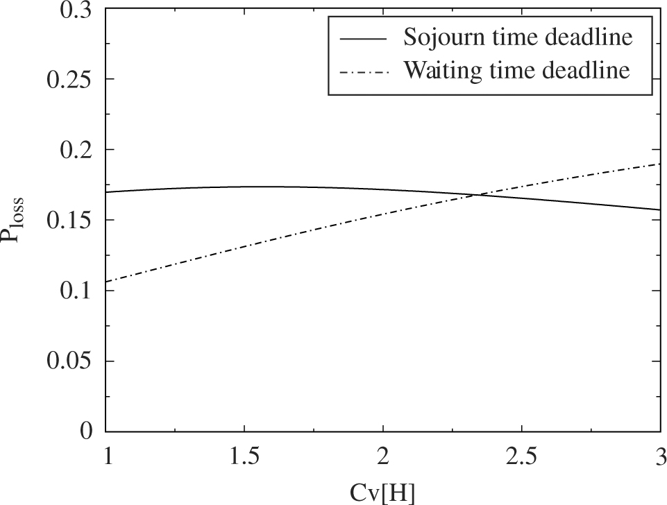
 $P_{{\rm{loss}}}^{\rm{w}}$ and
 $P_{{\rm{loss}}}^{\rm{s}}$ in the M/H2/1+M queue with λ = 0.7, E[H] = 1.0, and E[G] = 10.

Remark 7. Obviously, when service times follow an exponential distribution, 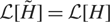 ${\cal L}[\tilde H] = {\cal L}[H]$ holds, so that (27) reduces to (24).
Remark 8. In the M/G/1+Mw queue,  $\pi _0^{\rm{w}}$ is explicitly given by [Reference Daley8, Reference Inoue and Takine9]
 $$\pi _0^{\rm{w}} = (1 + \sum\limits_{n = 1}^\infty {\rho ^n}\prod\limits_{k = 1}^{n - 1} {\cal L}[\tilde H](k\gamma {))^{ - 1}}.$$
 $P_{{\rm{loss}}}^{\rm{w}}$ is then obtained from (6), and we can compute
 $P_{{\rm{loss}}}^{\rm{s}}$ with (27) (cf. Remark 6).
In Figure 1 the loss probabilities in the M/H2/1+Mw and M/H2/1+Ms queues (with balanced hyper-exponential service times) are plotted as functions of the coefficient of variation Cv[H] of service times. We observe that  $P_{{\rm{loss}}}^{\rm{w}}$ monotonically increases as Cv[H] increases, which agrees with the theoretical result [Reference Inoue and Takine9] that in the M/G/1+Gw queue, the loss probability increases with the variability of service times in the convex order [Reference Shaked and Shanthikumar15, Equation (3.A.1)]. On the other hand, Figure 1 shows that
 $P_{{\rm{loss}}}^{\rm{s}}$ starts to decrease at some value of Cv[H], and as a result
 $P_{{\rm{loss}}}^{\rm{w}} \gt P_{{\rm{loss}}}^{\rm{s}}$ holds for large values of Cv[H], which provides a counterexample for
 $P_{{\rm{loss}}}^{\rm{w}} \le P_{{\rm{loss}}}^{\rm{s}}$.
4. Conclusion
We have discussed the relations between M/G/1+Gw and M/G/1+Gs queues. We first showed that the stationary distributions of the virtual waiting time, the actual waiting time, and the sojourn time in the M/G/1+Gs queue are given in terms of those in the corresponding M/G/1+Gw queue. With this result, we then derived comparison results between these models. Finally, we discussed two special cases: exponential service times (M/M/1+G) and exponential patience times (M/G/1+M).
Acknowledgement
This research was supported in part by JSPS KAKENHI grant number JP18K18007.