1. Introduction
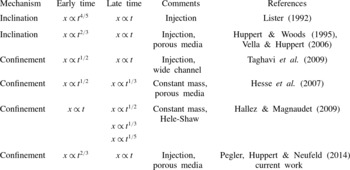
Fluid injection into a porous medium occurs in a large variety of geophysical and industrial processes such as seawater intrusion into coastal aquifers, geological sequestration of carbon dioxide, waste fluid disposal, and oil and gas recovery (e.g. Bear Reference Bear1972; Lake Reference Lake1989; Metz et al. Reference Metz, Davidson, De Connick, Loos and Meyer2005). When the injected and displaced fluids are immiscible, a free boundary problem can be formulated to describe the time evolution of the fluid–fluid interface (e.g. Huppert & Woods Reference Huppert and Woods1995; Nordbotten & Celia Reference Nordbotten and Celia2006; Zheng, Christov & Stone Reference Zheng, Christov and Stone2014). For such free boundary problems, there is often no fixed characteristic length scale in the direction of propagation. Therefore, during the propagation, the horizontal and vertical length scales may be different in the early and late time periods, and hence the solution may exhibit different asymptotic behaviours. In particular, even though the length scales are evolving, the shape of the interface at different times can be found through a transformation of independent variables, i.e. the gravity current may evolve in a self-similar fashion (Barenblatt Reference Barenblatt1979). Table 1 summarizes some typical situations when the propagation of a viscous gravity current exhibits a transition from an early time self-similarity to a distinct late time self-similarity.
Some typical physical situations when the propagation of a viscous gravity current exhibits a transition from an early time self-similar solution to another late time self-similar solution. We summarize the transition of the propagation law for the moving front of a gravity current in Cartesian coordinates. In this table,
 $x$
represents the length of the gravity current, and
 $t$
represents time. For fluid injection, we only summarize the results for constant injection from a line source, although the behaviour can possibly be extended to general power-law injection modes from either line or point sources.

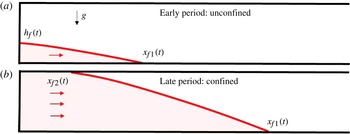
Fluid injection into a porous medium saturated with another fluid. The fluids are assumed immiscible, and the injected fluid (grey, red online) is denser than the displaced fluid (white). (a) For point source injection, the propagation is initially unconfined as the fluid–fluid interface only touches the bottom boundary, with
 $x_{f1}(t)$
denoting the location of the moving front at the bottom boundary;
 $h_{f}(t)$
denotes the location of the vertical tip. Both the length and the height of the injected fluid grow during the injection process. (b) As the height continues to increase, the propagation becomes confined, and the fluid–fluid interface eventually contacts the top boundary;
 $x_{f1}(t)$
still denotes the location of the moving front at the bottom boundary, while
 $x_{f2}(t)$
denotes the location of the moving front at the top boundary.

An example of a free boundary problem with distinct asymptotic limits in time is the release of a viscous fluid onto a slightly inclined plane. At early times, the gradient of the film thickness is large compared to the inclination angle, so the fluid spreads symmetrically. However, at longer times, i.e. the late time period, the flow is predominantly downslope as the effect of inclination becomes increasingly important (Lister Reference Lister1992). Similar time dependence at early and late times is found for the propagation of a gravity current along a tilted impermeable boundary in a porous medium (Huppert & Woods Reference Huppert and Woods1995; Vella & Huppert Reference Vella and Huppert2006), as well as for the problem that includes the effect of residual saturation (e.g. Hesse, Orr & Tchelepi Reference Hesse, Orr and Tchelepi2008; MacMinn, Szulczewski & Juanes Reference MacMinn, Szulczewski and Juanes2010, Reference MacMinn, Szulczewski and Juanes2011). Another example with distinct asymptotic limits is the post-injection movement of a buoyant fluid in a confined porous medium (Hesse et al. Reference Hesse, Tchelepi, Cantwell and Orr2007): initially, the fluid fills the entire depth of the porous medium; as the fluid spreads, the interface detaches from one boundary, and propagates predominantly along the other boundary, and the confinement associated with the detached boundary plays a decreasing role. In this situation, a transition from an early time similarity solution to a distinct late time similarity solution occurs. In fact, the post-injection spreading problem shares similar properties with the classic lock-exchange problem in a Hele-Shaw cell (e.g. Rottman & Simpson Reference Rottman and Simpson1983; Shin, Dalziel & Linden Reference Shin, Dalziel and Linden2004). Recently, Hallez & Magnaudet (Reference Hallez and Magnaudet2009) numerically investigated the lock-exchange problem, including the propagation of both high Reynolds number and low Reynolds number gravity currents, and demonstrated the transition processes from an early time slumping regime to different late time self-similar regimes found in previous studies (e.g. Huppert Reference Huppert1982b ; Huppert & Woods Reference Huppert and Woods1995). The effect of constant fluid injection on the lock-exchange problem in a wide channel has also been studied theoretically and numerically and a transition from an early time similarity solution to a late time compound wave solution for the fluid–fluid interface has been identified (Taghavi et al. Reference Taghavi, Seon, Martinez and Frigaard2009); related stability issues are also discussed in Taghavi et al. (Reference Taghavi, Alba, Seon, Wielage-Burchard, Martinez and Frigaard2012) and Saha, Salin & Talon (Reference Saha, Salin and Talon2013).
In this paper, we analyse the behaviour of a propagating interface when a fluid is injected into a confined porous medium saturated with another fluid in Cartesian coordinates, as shown in figure 1. Assuming the injected fluid is denser than the displaced fluid, then the injected fluid only attaches to the bottom boundary at early times for point source injection. As time progresses, the injected fluid contacts the top boundary, and the fluid flow becomes confined. As we show in this paper, during the propagation process, because of the change of the horizontal and vertical length scales, the solution exhibits a transition from an early time unconfined behaviour to a late time confined behaviour. In § 2, we set up the problem theoretically and derive a nonlinear convection–diffusion equation to describe the time evolution of the fluid–fluid interface. Then, we numerically solve the governing equation, together with appropriate boundary and initial conditions to show the time evolution of the fluid–fluid interface, which highlights the transition from an early time unconfined behaviour to a late time confined behaviour.
Motivated by the numerical results, in § 3 we provide two different scaling arguments, and identify a parabolic approximation of the governing equation in the early time period and a hyperbolic approximation in the late time period. Analytical solutions for both limiting equations are provided. In § 4, we provide two more analytical solutions in the late time period by including the diffusive term in the partial differential equation (PDE) due to buoyancy effects, which provide the structure of the moving front. Then, in § 5, we compare the numerical solutions with the analytical solutions for the time evolution of the fluid–fluid interface and the propagation law of the front, and show the transition processes between the early and late time regimes. In § 6, we identify the five distinct dynamical regimes (in the space of the dimensionless time and the viscosity ratio) for fluid injection into a confined porous medium and provide the approximate boundaries for each regime. We conclude this paper in § 7 by summarizing the main findings and discussing the model assumptions.
We note that, while we were finalizing our paper for submission, we learned of a recent publication by Pegler et al. (Reference Pegler, Huppert and Neufeld2014) that also analysed the problem we consider. Our analysis includes similar limits, but in the present work we have analysed the equation to characterize the flow regimes in which different approximate solutions are valid and we have illustrated the transitions between different asymptotic states representative of the injection process. More discussion about the work of Pegler et al. (Reference Pegler, Huppert and Neufeld2014) is provided in §§ 7.2 and 7.3.
2. Mathematical model and numerical investigation
2.1. The governing equation
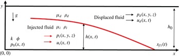
We are interested in the propagation of immiscible injected and displaced fluids in a porous medium, with
 $x$
and
 $y$
denoting the horizontal and vertical directions, respectively, as shown in figure 2. The porous medium with depth
 $h_{0}$
is assumed to be homogeneous and isotropic, with constant permeability
 $k$
and porosity
 ${\it\phi}$
. The injected fluid has a density
 ${\it\rho}_{i}$
and viscosity
 ${\it\mu}_{i}$
; the displaced fluid has a density
 ${\it\rho}_{d}$
and viscosity
 ${\it\mu}_{d}$
. We assume a sharp interface between the injected and displaced Newtonian fluids, with the shape of the fluid–fluid interface denoted by
 $h(x,t)$
; we also neglect the effect of surface tension at the interface. Without loss of generality, we assume the injected fluid is denser than the displaced fluid, i.e.
 ${\rm\Delta}{\it\rho}\equiv {\it\rho}_{i}-{\it\rho}_{d}>0$
; similar analysis applies to the case when the injected fluid is less dense than the displaced fluid, i.e.
 ${\rm\Delta}{\it\rho}<0$
.
Injection of a fluid into a homogeneous porous medium with constant permeability
 $k$
and porosity
 ${\it\phi}$
. The depth of the medium is denoted by
 $h_{0}$
. The injected fluid and the displaced fluid are immiscible, with a sharp interface
 $h(x,t)$
between them. In this diagram, the injected fluid is assumed denser than the displaced fluid, i.e.
 ${\it\rho}_{i}>{\it\rho}_{d}$
.
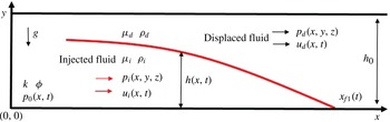
To analyse the flow, we assume that the fluid–fluid interface is long and thin, so that the lubrication approximation holds, and the vertical velocity can be neglected. In this case, the fluids in the porous medium exhibit hydrostatic pressure distributions:
 $$\begin{eqnarray}\displaystyle p_{i}(x,y,t) & = & \displaystyle p_{0}(x,t)-{\it\rho}_{i}gy,\quad \text{for}~y\leqslant h(x,t),\end{eqnarray}$$
 $$\begin{eqnarray}\displaystyle p_{d}(x,y,t) & = & \displaystyle p_{0}(x,t)-{\it\rho}_{i}gh(x,t)-{\it\rho}_{d}g(y-h(x,t)),\quad \text{for}~y>h(x,t),\end{eqnarray}$$
 $p_{i}(x,y,t)$
and
 $p_{d}(x,y,t)$
denote the pressure in the injected and displaced fluid, respectively;
 $p_{0}(x,t)$
represents the pressure at the impermeable bottom boundary. Then, the horizontal velocities of the injected fluid
 $u_{i}(x,t)$
and the displaced fluid
 $u_{d}(x,t)$
can be calculated using Darcy’s law:
 $$\begin{eqnarray}u_{i}(x,t)=-\frac{k}{{\it\mu}_{i}}\frac{\partial p_{i}}{\partial x}\quad \text{and}\quad u_{d}(x,t)=-\frac{k}{{\it\mu}_{d}}\frac{\partial p_{d}}{\partial x}.\end{eqnarray}$$
One-dimensional continuity equations can be written for both the injected and displaced fluids:
 $$\begin{eqnarray}{\it\phi}\frac{\partial h}{\partial t}+\frac{\partial (hu_{i})}{\partial x}=0,\quad {\it\phi}\frac{\partial (h_{0}-h)}{\partial t}+\frac{\partial ((h_{0}-h)u_{d})}{\partial x}=0.\end{eqnarray}$$
Adding the latter together provides a global conservation of mass equation:
 $$\begin{eqnarray}q=hu_{i}+(h_{0}-h)u_{d},\end{eqnarray}$$
where
 $q$
denotes the volumetric injection rate. When fluid is injected at a constant rate,
 $q$
is constant. Assuming fluid injection begins at
 $t=0$
, the global mass conservation equation (2.4) can be re-written in an equivalent form, as a constraint,
 $$\begin{eqnarray}{\it\phi}\int _{0}^{x_{f1}(t)}h(x,t)\text{d}x=qt,\end{eqnarray}$$
with
 $x_{f1}(t)$
denoting the propagating front at the bottom boundary, beyond which
 $h=0$
.
After some rearrangement of (2.1)–(2.4), we obtain a nonlinear convection–diffusion equation for the height of the current (Bear Reference Bear1972):
 $$\begin{eqnarray}{\it\phi}\frac{\partial h}{\partial t}+qM\frac{\partial }{\partial x}\left[\frac{h}{(M-1)h+h_{0}}\right]-\frac{{\rm\Delta}{\it\rho}gk}{{\it\mu}_{i}}\frac{\partial }{\partial x}\left[\frac{h(h_{0}-h)}{(M-1)h+h_{0}}\frac{\partial h}{\partial x}\right]=0,\end{eqnarray}$$
where
 $M\equiv {\it\mu}_{d}/{\it\mu}_{i}$
denotes the ratio of the viscosity of the displaced fluid to the viscosity of the injected fluid. Equation (2.6) describes the time evolution of the fluid–fluid interface. The special case of (2.6) with
 $M=1$
is given in, e.g. Bear (Reference Bear1972) and Huppert & Woods (Reference Huppert and Woods1995), and the axisymmetric form of (2.6) is given by Nordbotten & Celia (Reference Nordbotten and Celia2006).
2.2. Initial and boundary conditions
We assume that the fluid injection occurs for
 $t\geqslant 0$
. Before the injection, only the displaced fluid fills the porous medium. Thus, the initial condition for the problem is
 $$\begin{eqnarray}h(x,0)=0.\end{eqnarray}$$
Now we state the appropriate boundary conditions for this problem. We note that at the moving front along the lower boundary, i.e.
 $x=x_{f1}(t)$
, the boundary condition is
 $$\begin{eqnarray}h(x_{f1}(t),t)=0.\end{eqnarray}$$
We can also integrate (2.6) from
 $x=0$
to
 $x=x_{f1}(t)$
, which gives
 $$\begin{eqnarray}{\it\phi}\int _{0}^{x_{f1}(t)}\frac{\partial h}{\partial t}\text{d}x+\left[\frac{qMh}{(M-1)h+h_{0}}-\frac{{\rm\Delta}{\it\rho}gk}{{\it\mu}_{i}}\frac{h(h_{0}-h)}{(M-1)h+h_{0}}\frac{\partial h}{\partial x}\right]_{0}^{x_{f1}(t)}=0.\end{eqnarray}$$
Substituting the global mass constraint (2.5) and the boundary condition at the front, i.e. (2.8), equation (2.9) can be rewritten as
 $$\begin{eqnarray}\left.\left[\frac{qMh}{(M-1)h+h_{0}}-\frac{{\rm\Delta}{\it\rho}gk}{{\it\mu}_{i}}\frac{h(h_{0}-h)}{(M-1)h+h_{0}}\frac{\partial h}{\partial x}\right]\right|_{x=0}=q,\end{eqnarray}$$
which provides a boundary condition at
 $x=0$
. Note that all solutions we consider obey
 $\lim _{x\rightarrow x_{f1}}h(\partial h/\partial x)=0$
.
Equations (2.7), (2.8) and (2.10) serve as the initial and boundary conditions for the point source fluid injection problem. It should be noted that the governing equation (2.6), together with the initial and boundary conditions, i.e. (2.7), (2.8) and (2.10), do not change after the fluid–fluid interface attaches to the top boundary, as shown in figure 1, though after this event we also keep track of the moving front
 $x_{f2}(t)$
along the upper boundary.
2.3. Non-dimensionalization
For a confined porous medium, a characteristic vertical length scale is the depth of the porous medium
 $h_{0}$
. We start by rewriting (2.6) using dimensionless variables
 $H=h/h_{c}$
,
 $X=x/x_{c}$
,
 $T=t/t_{c}$
, where
 $$\begin{eqnarray}h_{c}=h_{0},\quad x_{c}=\frac{{\rm\Delta}{\it\rho}gkh_{0}^{2}}{{\it\mu}_{i}q},\quad t_{c}=\frac{{\rm\Delta}{\it\rho}gk{\it\phi}h_{0}^{3}}{{\it\mu}_{i}q^{2}}.\end{eqnarray}$$
With these definitions we obtain a dimensionless form of (2.6):
 $$\begin{eqnarray}\frac{\partial H}{\partial T}+\frac{\partial }{\partial X}\left[\frac{MH}{(M-1)H+1}\right]-\frac{\partial }{\partial X}\left[\frac{H(1-H)}{(M-1)H+1}\frac{\partial H}{\partial X}\right]=0,\end{eqnarray}$$
where
 $M\equiv {\it\mu}_{d}/{\it\mu}_{i}$
is the only dimensionless parameter. The initial and boundary conditions can also be rewritten using the dimensionless variables:
 $$\begin{eqnarray}\displaystyle H(X,0) & = & \displaystyle 0,\end{eqnarray}$$
 $$\begin{eqnarray}\displaystyle H(X_{f1}(T),T) & = & \displaystyle 0,\end{eqnarray}$$
 $$\begin{eqnarray}\displaystyle \left.\left[\frac{MH}{(M-1)H+1}-\frac{H(1-H)}{(M-1)H+1}\frac{\partial H}{\partial X}\right]\right|_{X=0} & = & \displaystyle 1,\end{eqnarray}$$
 $X_{f1}(T)\equiv x_{f1}(t)/x_{c}$
denotes the dimensionless location of the front at the bottom boundary.
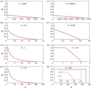
Numerical simulations of the injection of a denser fluid into a confined porous medium saturated with another fluid, assuming the injected and displaced fluids are immiscible.
 $M$
denotes the ratio of the viscosity of the displaced fluid to that of the injected fluid. (a–d)
 $M>1$
(
 $M=5$
), i.e. the injected fluid is less viscous than the displaced fluid. (e–h)
 $M<1$
(
 $M=1/2$
), i.e. the injected fluid is more viscous than the displaced fluid. In both cases, in the early time period the fluid–fluid interface only attaches to the bottom boundary, while in the late time period the interface attaches to both the top and the bottom boundaries. Inset of (h): with
 $M<1$
, the fluid–fluid interface appears to have a linear spatial structure in the late time period. Note that the horizontal length scales are different in each plot.

2.4. Numerical simulation
We conducted direct numerical simulations of the nonlinear convection–diffusion equation (2.12), with boundary and initial conditions given by (2.13), using the finite-difference scheme of Kurganov & Tadmor (Reference Kurganov and Tadmor2000). The details of the numerical procedure are discussed in appendix A. Typical numerical results are shown in figure 3. Specifically, the numerical simulations span a wide range of time. In addition, different values of
 $M$
are used in these simulations, including
 $M>1$
,
 $M=1$
and
 $M<1$
.
First, we show examples when the denser injected fluid is less viscous than the displaced fluid (i.e.
 $M>1$
) in figure 3(a–d). In the early time period for point source injection, the fluid–fluid interface only touches the bottom boundary at
 $X=X_{f1}(T)$
, and the propagation is unconfined. As injection continues, both the length and the height of the fluid–fluid interface grow, and the interface eventually touches the top boundary, creating a second moving front at
 $X=X_{f2}(T)$
along the top boundary of the porous medium. The numerical simulations suggest that the two fronts propagate in the late time period with constant but distinct speeds.
Second, we show examples when the injected fluid has a viscosity higher than or equal to that of the displaced fluid (i.e.
 $M\leqslant 1$
) in figure 3(e–h). Again, in the early time period, the fluid–fluid interface only contacts the bottom boundary; later, the interface contacts the top boundary, and forms a second front
 $X_{f2}(T)$
. In the late time period, the shape of the fluid–fluid interface appears similar to the shape of a shock wave, and both the top and bottom fronts appear to propagate at the same constant speed. If we examine the shape near the propagating fronts, we observe that the fluid–fluid interface is not precisely a (discontinuous) shock wave. Instead, the front has a linear spatial structure, with a slope of
 $-$
2, for example, for
 $M=1/2$
, as shown in the inset of figure 3(h). Further discussion in § 4 shows that the slope of the interface is the constant
 $1/(M-1)$
for
 $M<1$
, while the slope increases in time for
 $M=1$
.
3. Early time and late time approximate solutions
The numerical results motivate us to look for approximate solutions in the early and late time periods. The dimensionless form of the governing equation (2.12) suggests that when
 $T=\text{ord}(1)$
, the convective and the diffusive terms have the same order of magnitude. Thus, they both play an important role in the solution
 $H(X,T)$
, which represents the time evolution of the fluid–fluid interface. The notation
 $\text{ord}(1)$
denotes terms strictly of order unity (Hinch Reference Hinch1991). (Note that, for example, while
 ${\it\epsilon}^{n}=O({\it\epsilon}^{m})$
as
 ${\it\epsilon}\rightarrow 0$
for any
 $0<m\leqslant n$
and
 ${\it\epsilon}^{n}=o({\it\epsilon}^{m})$
for any
 $0<m<n$
,
 ${\it\epsilon}^{n}=\text{ord}({\it\epsilon}^{m})$
only for
 $m=n$
, which then allows us to use
 ${>}$
and
 ${<}$
signs with respect to
 $\text{ord}(\cdot )$
for
 $m\neq n$
.)
However, as time progresses, the convective and diffusive terms can have different orders of magnitude, since the characteristic scales for the length
 $X_{c}(T)$
and the height
 $H_{c}(T)$
of the current can change significantly. Specifically, numerical results in § 2.4, e.g. figure 3, suggest that in the early time period the diffusive term is dominant, while in the late time period the convective term is dominant. We discuss the dynamics in the early time period in § 3.1 and that in the late time period in § 3.2. Estimates of the early and late time periods are provided at the end of each section.
3.1. The early time period
For injection from a point source, in the early time period, the flow is unconfined. The fluid–fluid interface only contacts the bottom boundary; both the length and the height of the injected fluid increase throughout this period.
A posteriori we claim that, in the early time period, the full governing equation (2.12) can be reduced to a nonlinear diffusion equation, which describes the propagation of gravity currents in an unconfined porous medium (e.g. Boussinesq Reference Boussinesq1904; Barenblatt Reference Barenblatt1979; Huppert & Woods Reference Huppert and Woods1995; Zheng et al. Reference Zheng, Christov and Stone2014):
 $$\begin{eqnarray}\frac{\partial H}{\partial T}=\frac{\partial }{\partial X}\left(H\frac{\partial H}{\partial X}\right)\!.\end{eqnarray}$$
Physically, during this early time period, the upper boundary plays no role in the propagation of the fluid–fluid interface; the pressure gradient for the fluid motion is provided by the buoyancy force, and the pressure gradient associated with injection is negligible.
Next, the global mass constraint (2.5) can be rewritten as
 $$\begin{eqnarray}\int _{0}^{X_{f1}(T)}H(X,T)\text{d}X=T.\end{eqnarray}$$
Equations (3.1) and (3.2) possess a well-known self-similar solution that describes the time evolution of the fluid–fluid interface (e.g. Huppert & Woods Reference Huppert and Woods1995).
To construct this self-similar solution, we define a similarity variable
 ${\it\xi}\equiv X/T^{2/3}$
; thus, the front propagates according to
 $X_{f1}(T)={\it\xi}_{f}T^{2/3}$
, where
 ${\it\xi}_{f}$
is a constant to be determined. We then introduce
 $s\equiv X/X_{f1}(T)={\it\xi}(X,T)/{\it\xi}_{f}$
, so that the shape of the interface can be expressed as
 $H(X,T)={\it\xi}_{f}^{2}T^{1/3}f(s)$
. Here
 $f(s)$
and
 ${\it\xi}_{f}$
are the solution of the system
 $$\begin{eqnarray}\displaystyle (\,f\,f^{\prime })^{\prime }+{\textstyle \frac{2}{3}}s\,f^{\prime }-{\textstyle \frac{1}{3}}\,f & = & \displaystyle 0,\end{eqnarray}$$
 $$\begin{eqnarray}\displaystyle f(1) & = & \displaystyle 0,\end{eqnarray}$$
 $$\begin{eqnarray}\displaystyle {\it\xi}_{f} & = & \displaystyle \left(\int _{0}^{1}f(s)\text{d}s\right)^{-1/3},\end{eqnarray}$$
 $s$
. We can determine the asymptotic behaviour near the front of the interface based on (3.3a
,
b
):
 $$\begin{eqnarray}f(s)\sim {\textstyle \frac{2}{3}}(1-s)\quad \text{as}~s\rightarrow 1^{-}.\end{eqnarray}$$
Equation (3.4) provides two boundary conditions near the front
 $s=1$
, i.e.
 $f(1-{\it\lambda})$
and
 $f^{\prime }(1-{\it\lambda})$
with
 ${\it\lambda}\ll 1$
, which can be used in a shooting procedure for numerically solving (3.3a
). The numerically computed shape
 $f(s)$
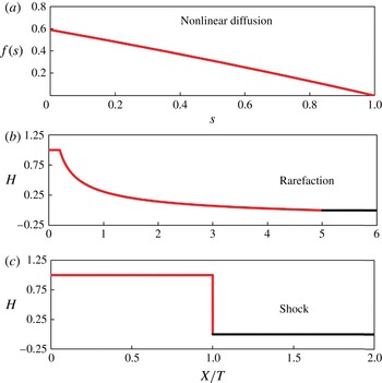
is shown in figure 4(a), and the value of the pre-factor is
 ${\it\xi}_{f}\approx 1.48$
. Thus, we have obtained a self-similar solution for the nonlinear diffusion problem; the front attached to the bottom boundary propagates as
 $X_{f1}(T)\approx 1.48T^{2/3}$
; the vertical tip, i.e. the height of the interface at the injection point
 $X=0$
, grows as
 $H_{f}(T)\equiv H(0,T)\approx 1.30T^{1/3}$
. These calculations are consistent with previous studies (e.g. Huppert & Woods Reference Huppert and Woods1995).
The analytical solutions in the different asymptotic limits. (a) The self-similar solution to the nonlinear diffusion system (3.1) and (3.2); this solution is independent of
 $M$
and holds in the early time period. (b) The rarefaction wave solution (3.9) to the hyperbolic equation (3.6) with
 $M=5$
. (c) The shock solution (3.12) to the hyperbolic equation (3.6) with
 $M=1/2$
. The shock and rarefaction solutions hold in the late time period.

Let us now provide an estimate for the early time period, when the full equation (2.12) can be reduced to the nonlinear diffusion equation (3.1). A more formal discussion is provided in appendix B. Note that in the early time period, the appropriate length scale is the location of the front attached to the bottom boundary, i.e.
 $X_{c}(T)\approx X_{f1}(T)\propto T^{2/3}$
, while the height scale can be chosen to be the location of the vertical tip, i.e.
 $H_{c}(T)\approx H_{f}(T)\propto T^{1/3}$
.
We first need the convective term to be negligible compared with the diffusive term in (2.12), i.e.
 $MX_{c}/(H_{c}(1-H_{c}))\ll 1$
. Substituting in
 $X_{c}(T)=T^{2/3}$
and
 $H_{c}(T)=T^{1/3}$
, we obtain
 $M^{-1}(T^{-1/3}-1)\geqslant \text{ord}({\it\epsilon}^{-1})$
, where
 ${\it\epsilon}\ll 1$
is an arbitrary small number, the notation
 $\text{ord}({\it\epsilon}^{-1})$
denotes terms strictly of order
 ${\it\epsilon}^{-1}$
, and
 ${\geqslant}$
with regard to
 $\text{ord}(\cdot )$
is then used in the sense of Hinch (Reference Hinch1991) as before. With the convective term negligible, when
 $M\gg 1$
, we further require
 $MH_{c}\ll 1$
to reduce (2.12) to the nonlinear diffusion equation (3.1). Thus, we obtain
 $MT^{1/3}\ll 1$
with
 $M\gg 1$
. Note that
 $M^{-1}(T^{-1/3}-1)\geqslant \text{ord}({\it\epsilon}^{-1})$
is a stricter requirement than
 $MT^{1/3}\leqslant \text{ord}({\it\epsilon})$
.
Thus, we obtain an estimate for the early time period:
 $M^{-1}(T^{-1/3}-1)\geqslant \text{ord}({\it\epsilon}^{-1})$
. The value of
 ${\it\epsilon}\ll 1$
is arbitrary, which then determines how close the approximation is to the full problem. In this early time period, the leading-order terms of (2.12) become the nonlinear diffusion equation (3.1). It should be noted that this estimate is based on analysing the behaviour of the governing equations, and it does not include an estimate for the transition period, i.e. how long it takes to develop a self-similar solution from a given initial condition. A direct comparison of the self-similar solution from (3.3) with a numerical solution is necessary to provide a precise crossover time, including the influence of the transition period.
3.2. The late time period
In the late time period, the fluid flow is confined, and the fluid–fluid interface attaches to both the top and the bottom boundaries, and
 $X_{f1}(T)$
and
 $X_{f2}(T)$
denote the location of the fronts, respectively:
 $$\begin{eqnarray}\displaystyle H(X_{f1}(T),T) & = & \displaystyle 0,\end{eqnarray}$$
 $$\begin{eqnarray}\displaystyle H(X_{f2}(T),T) & = & \displaystyle 1.\end{eqnarray}$$
A posteriori we claim that the diffusive term is negligible compared with the convective term in (2.6) in the late time period for the majority of the flow, and that for point source injection the equation for the shape of the current is approximated by a nonlinear hyperbolic equation:
 $$\begin{eqnarray}\frac{\partial H}{\partial T}+\frac{\partial }{\partial X}\left(\frac{MH}{(M-1)H+1}\right)=0.\end{eqnarray}$$
Physically, in this late time period, the pressure gradient for the fluid motion is provided by injection, with the buoyancy force being negligible.
Given appropriate boundary and initial conditions, (3.6) can be solved using the method of characteristics. Specifically, the flux boundary condition (2.13c
) can be rewritten as
 $H(0,T)=1$
as the boundary condition for (3.6), since the interface attaches to both the top and the bottom boundaries in the late time period. The initial condition can be provided by solving (2.12) numerically with boundary and initial conditions given by (2.13) until the ‘beginning’ of the late time period, as we define at the end of this section.
Even without specifying an initial condition for (3.6), we can discuss the generic properties of its solutions. Since (3.6) is a scalar equation with a convex flux function,
 $$\begin{eqnarray}F(H)\equiv \frac{MH}{(M-1)H+1},\end{eqnarray}$$
the theory of hyperbolic conservation laws (e.g. LeVeque Reference LeVeque2002) suggests only two possible ways in which an initial condition satisfying (3.5) can evolve: into a shock wave or into a rarefaction wave. The derivative of the flux function,
 $F^{\prime }(H)$
, determines the local wave speed. Thus, if
 $F^{\prime }(1)>F^{\prime }(0)$
, where we have assumed that any solution of (3.6) in this limit will connect the left and right states
 $H=1$
and
 $H=0$
, respectively, the initial condition becomes double-valued beyond a certain critical time determined, in part, by the difference
 $X_{f1}(T)-X_{f2}(T)$
at the instant
 $T$
at which the initial condition is imposed. On the other hand, if
 $F^{\prime }(1)<F^{\prime }(0)$
, then the initial condition ‘spreads’ and evolves into a rarefaction wave.
Rarefaction waves are, by construction, self-similar solutions
 $H(X,T)=H({\it\zeta})$
in terms of the similarity variable
 ${\it\zeta}\equiv X/T$
. Substituting
 $H({\it\zeta})$
into (3.6), we obtain
 $$\begin{eqnarray}\frac{\text{d}H}{\text{d}{\it\zeta}}\left(\frac{\text{d}F}{\text{d}H}-{\it\zeta}\right)=0.\end{eqnarray}$$
The rarefaction wave is a non-trivial solution, hence
 $\text{d}H/\text{d}{\it\zeta}\neq 0$
everywhere, and (3.8) reduces to
 $\text{d}F/\text{d}H={\it\zeta}$
, which has the solution
 $$\begin{eqnarray}H(X,T)=\left\{\begin{array}{@{}ll@{}}1,\quad & X/T\leqslant 1/M,\\ \left(\sqrt{M/(X/T)}-1\right)/(M-1),\quad & 1/M<X/T\leqslant M,\\ 0,\quad & X/T>M.\end{array}\right.\end{eqnarray}$$
An example rarefaction wave solution is shown in figure 4(b) with
 $M=5$
. It should be noted that the rarefaction wave solution for similar problems has been reported previously (e.g. Nordbotten & Celia Reference Nordbotten and Celia2006; Verdon & Woods Reference Verdon and Woods2007; Gunn & Woods Reference Gunn and Woods2011). As stated earlier, a given initial condition will always evolve into a rarefaction wave under (3.6) if
 $F^{\prime }(1)<F^{\prime }(0)$
or, equivalently,
 $M>1$
. Furthermore, from (3.9), we can show that the front along the bottom boundary is located at
 $X_{f1}(T)=MT$
, while the front along the top boundary is located at
 $X_{f2}(T)=T/M$
. Clearly,
 $X_{f2}(T)$
propagates slower than
 $X_{f1}(T)$
since we have assumed
 $M>1$
.
On the other hand, for
 $F^{\prime }(1)>F^{\prime }(0)$
, or equivalently
 $M<1$
, we must seek a weak solution of (3.6) in the form of a discontinuity (i.e. a shock), connecting the states
 $H=1$
and
 $H=0$
, at some location
 $X_{s}(T)$
. The location of the shock
 $X_{s}(T)$
can be determined by integrating the shock speed relation provided by the Rankine–Hugoniot condition (e.g. LeVeque Reference LeVeque2002):
 $$\begin{eqnarray}\frac{\text{d}X_{s}}{\text{d}T}=\frac{F\left(H\left(X_{s}^{-},T\right)\right)-F\left(H\left(X_{s}^{+},T\right)\right)}{H\left(X_{s}^{-},T\right)-H\left(X_{s}^{+},T\right)}=F(1)-F(0)=1.\end{eqnarray}$$
Hence,
 $X_{s}(T)=T$
, assuming
 $X_{s}(0)=0$
. Since weak solutions are, in general, not unique, we must verify that a shock with speed given by (3.10) is an entropy-satisfying weak solution of the conservation law (3.6). To do so, we apply the Lax entropy condition (e.g. LeVeque Reference LeVeque2002):
 $$\begin{eqnarray}F^{\prime }\left(H\left(X_{s}^{-},T\right)\right)>\frac{\text{d}X_{s}}{\text{d}T}>F^{\prime }\left(H\left(X_{s}^{+},T\right)\right)\!.\end{eqnarray}$$
Since, for
 $M<1$
,
 $F^{\prime }(H)$
is a monotonically increasing function with minimum at
 $(H,F^{\prime })=(0,0)$
and maximum at
 $(H,F^{\prime })=(1,1/M)$
, the inequality (3.11) is always satisfied for the shock speed (3.10). Thus, the shock solution
 $$\begin{eqnarray}H(X,T)=\left\{\begin{array}{@{}ll@{}}1,\quad & X/T\leqslant 1,\\ 0,\quad & X/T>1\end{array}\right.\end{eqnarray}$$
is the unique entropy-satisfying weak solution to (3.6) for
 $M<1$
; a similar argument shows that this is not true for
 $M>1$
. In this case, the front along the bottom boundary
 $X_{f1}(T)$
and the front along the top boundary
 $X_{f2}(T)$
coincide and propagate at the shock speed, i.e.
 $X_{f1}(T)=X_{f2}(T)=X_{s}(T)=T$
. An example shock solution is shown in figure 4(c) with
 $M=1/2$
.
We note that the shock solution (3.12) ends abruptly at the front of the current
 $X_{f1}(T)=X_{f2}(T)=T$
, which is different from the solution observed in figure 3(h). This difference is because the hyperbolic equation (3.6) is a singular perturbation of (2.12), i.e. we have neglected the highest derivative in
 $X$
. In § 4.1, we provide a travelling wave solution for
 $M<1$
in the late time period for the full equation (2.12). This solution provides the structure of the fluid–fluid interface. However, the shock solution (3.12) of (3.6) describes the majority of the spatial extent of the flow, in particular, the global spreading rate. Similar situations are also manifested in the solution to related hyperbolic equations describing the shape of viscous gravity currents down a slope (e.g. Huppert Reference Huppert1982a
; Lister Reference Lister1992; Vella & Huppert Reference Vella and Huppert2006). It should also be noted that in (3.12), as in (3.9), we have neglected any transient behaviour in the solution due to the details of the initial condition since we are only concerned with the generic properties of solutions to the hyperbolic equation (3.6).
Thus, we have identified a rarefaction wave solution (3.9) for
 $M>1$
and a shock solution (3.12) for
 $M<1$
in the late time period by studying the hyperbolic equation (3.6). For the special case of
 $M=1$
, equation (3.6) is reduced to
 $$\begin{eqnarray}\frac{\partial H}{\partial T}+\frac{\partial H}{\partial X}=0.\end{eqnarray}$$
The solution is
 $H_{0}(X-T)$
, where
 $H_{0}$
denotes the ‘initial’ shape in the late time period. This solution suggests that the fluid–fluid interface propagates with a constant speed equal to the shock speed
 $\text{d}X_{s}/\text{d}T=1$
, while maintaining the ‘initial’ shape. In § 4.2, we provide another analytical solution for
 $M=1$
in the late time period by solving (2.12) using a self-similar transformation, which includes both the convective and the diffusive terms.
Let us now provide an estimate for the late time period when the shock solution (3.12) and the rarefaction wave solution (3.9) become good approximations to solution to the full equation (2.12). We first need the interface to attach to the top boundary, which requires
 $T\geqslant 1$
. In addition, we require that the diffusive term is negligible compared with the convective term.
When
 $M<1$
, the shock solution (3.12) suggests that the interface propagates at the shock speed
 $\text{d}X_{s}/\text{d}T=1$
. Thus, the appropriate length scale is
 $X_{c}=X_{s}(T)=T$
, which suggests that for the diffusive term to be negligible we need
 $MX_{c}=MT\gg 1$
. Thus, we obtain an estimate of a time scale beyond which the hyperbolic equation (3.6) approximates the full equation (2.12):
 $MT\geqslant \text{ord}({\it\epsilon}^{-1})$
.
When
 $M>1$
, the rarefaction wave solution (3.9) suggests different behaviours near the bottom and top boundaries: substituting (3.9) into the full equation (2.12), near the bottom boundary (
 $X\rightarrow MT$
), the ratio of the convective term compared with the diffusive term is
 $2T(M-1)M^{2}$
, while near the top boundary (
 $X\rightarrow T/M$
), the ratio is
 $2T(M-1)/M$
. Therefore, we need
 $T(M-1)M^{2}\geqslant \text{ord}({\it\epsilon}^{-1})$
for the hyperbolic equation (3.6) to provide a good approximation near the bottom boundary, while we require
 $T(M-1)/M\geqslant \text{ord}({\it\epsilon}^{-1})$
for (3.6) to give a good approximation near the top boundary. Again, it should be noted that our estimate is based on analysing the governing equations and does not include an estimate for the transition period for the rarefaction solution (3.9) to develop from a given initial condition.
4. Late time self-similar intermediate asymptotics for (2.12)
In § 3.2, in order to derive (3.6) from (2.12), we have neglected the diffusive term in the late time period. In this section, we provide two more analytical solutions to the full equation (2.12) in the late time period, when the fluid–fluid interface contacts both the top and the bottom boundaries. The analytical solutions to the full equation (2.12) include the diffusive term due to buoyancy effects, and provide the structure of the fluid–fluid interface. In addition, these solutions represent the intermediate asymptotics of (2.12), hence all solutions hold after the initial condition is forgotten and the interface attaches to both boundaries, i.e. in the late time period. Specifically, we provide a travelling wave solution for
 $M<1$
in § 4.1, and a self-similar solution for
 $M=1$
in § 4.2. These analytical solutions of (2.12) provide the structure of the fluid–fluid interface.
4.1. Travelling wave solution for
 $M<1$

Let us consider the case of
 $M<1$
. A shock solution (3.12) was obtained as an approximation of the time evolution of the fluid–fluid interface from the hyperbolic equation (3.6). We now consider the fluid–fluid interface in a coordinate system moving with the location of the shock front. We define a new variable
 ${\it\zeta}_{c}\equiv X-T$
, and assume that
 $H(X,T)$
is a function of
 ${\it\zeta}_{c}$
only, i.e.
 $H=H({\it\zeta}_{c})$
. The subscript ‘
 $c$
’ indicates that we are looking for the correction from the diffusive term at the shock front. Equation (2.12) can be rewritten as an ordinary differential equation (ODE) in terms of
 ${\it\zeta}_{c}$
:
 $$\begin{eqnarray}-\frac{\text{d}H}{\text{d}{\it\zeta}_{c}}+\frac{\text{d}}{\text{d}{\it\zeta}_{c}}\left(\frac{MH}{(M-1)H+1}\right)-\frac{\text{d}}{\text{d}{\it\zeta}_{c}}\left(\frac{H(1-H)}{(M-1)H+1}\frac{\text{d}H}{\text{d}{\it\zeta}_{c}}\right)=0.\end{eqnarray}$$
We seek a solution with two moving fronts, which leads to the conditions
 $$\begin{eqnarray}\displaystyle H\left({\it\zeta}_{c,f1}\right) & = & \displaystyle 0,\end{eqnarray}$$
 $$\begin{eqnarray}\displaystyle H\left({\it\zeta}_{c,f2}\right) & = & \displaystyle 1,\end{eqnarray}$$
 ${\it\zeta}_{c,f1}$
and
 ${\it\zeta}_{c,f2}$
represent the location of the moving fronts which attach to the bottom and top boundaries, respectively. Note that these are unknown and are determined as part of the problem.
Integrating (4.1) once, and using condition (4.2a ) to set the integration constant to zero, we obtain, after some rearrangement,
 $$\begin{eqnarray}\frac{\text{d}H}{\text{d}{\it\zeta}_{c}}=M-1.\end{eqnarray}$$
Equation (4.3) indicates that the moving interface has a linear structure at the front. Using the global mass constraint, we find
 $$\begin{eqnarray}H({\it\zeta}_{c})=(M-1)\left({\it\zeta}_{c}+\frac{1}{2(M-1)}\right).\end{eqnarray}$$
The locations of the moving fronts are obtained by setting
 $H=1$
and
 $H=0$
:
 ${\it\zeta}_{c,f2}=1/(2(M-1))$
for the front that attaches to the top boundary
 $(H=1)$
, and
 ${\it\zeta}_{c,f1}=-1/(2(M-1))$
for the front that attaches to the bottom boundary
 $(H=0)$
. The thickness of the linear structure of the moving interface is
 ${\it\zeta}_{c,f1}-{\it\zeta}_{c,f2}=1/(1-M)$
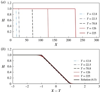
. An example of this solution is shown (black solid line) in figure 5(b) for
 $M=1/2$
.
Numerical solutions for the time evolution of the fluid–fluid interface with
 $M=1/2$
in the late time period. (a) Over a long length scale, the interface appears similar to a shock wave, a heuristic approximation. (b) However, in the neighborhood of the propagating front, the interface has a linear structure in the moving frame. The travelling wave solution (4.5) is also plotted in (b), showing that it agrees well with the numerical solutions.

Thus, the complete structure of the fluid–fluid interface in the late time period with
 $M<1$
is given by
 $$\begin{eqnarray}H(X,T)=\left\{\begin{array}{@{}ll@{}}1,\quad & X\leqslant T+1/(2(M-1)),\\ (M-1)(X-T)+1/2,\quad & T+1/(2(M-1))<X\leqslant T-1/(2(M-1)),\\ 0,\quad & X>T-1/(2(M-1)).\end{array}\right.\end{eqnarray}$$
The travelling wave solution given by (4.5) agrees very well with the numerical solution to (2.12) in the late time period, as shown in figure 5. Both the front locations and the structure of the fluid–fluid interface are captured. It should also be noted that as the length of the injected fluid continues to grow, the ratio of the thickness of the fixed linear structure relative to the length of the injected fluid continues to decrease. Thus, the discontinuous shock solution (3.12) evolves as a heuristic approximation of the late time evolution of the fluid–fluid interface. In addition, solution (4.5) holds when the interface attaches to both the top and bottom boundaries, which requires
 $X_{f2}(T)=T+1/(2(M-1))>0$
. Thus, we obtain a crossover time scale when the solution in (4.5) provides a good approximation:
 $T(1-M)\geqslant \text{ord}(1)$
.
4.2. Self-similar solution for
$M=1$

When the injected and the displaced fluids have equal viscosities, i.e.
 $M=1$
, the solution (4.5) does not apply. However, as we show in this section, we can obtain another self-similar solution to (2.12) with
 $M=1$
, including the effects of both the convective and diffusive terms.
Substituting
 $M=1$
into (2.12), we obtain
 $$\begin{eqnarray}\frac{\partial H}{\partial T}+\frac{\partial H}{\partial X}-\frac{\partial }{\partial X}\left(H(1-H)\frac{\partial H}{\partial X}\right)=0.\end{eqnarray}$$
We seek a self-similar solution
 $H(X,T)=H({\it\zeta}_{e})$
in terms of the similarity variable
 ${\it\zeta}_{e}\equiv (X-T)/T^{1/2}$
. Here the subscript ‘
 $e$
’ denotes that we are looking for a solution when the injected and displaced fluids have equal viscosities. After some rearrangements, (4.6) is reduced to an ODE:
 $$\begin{eqnarray}\frac{1}{2}{\it\zeta}_{e}\frac{\text{d}H}{\text{d}{\it\zeta}_{e}}+\frac{\text{d}}{\text{d}{\it\zeta}_{e}}\left(H(1-H)\frac{\text{d}H}{\text{d}{\it\zeta}_{e}}\right)=0.\end{eqnarray}$$
The appropriate front conditions are
 $$\begin{eqnarray}\displaystyle & H({\it\zeta}_{e,f1})=0, & \displaystyle\end{eqnarray}$$
 $$\begin{eqnarray}\displaystyle & H({\it\zeta}_{e,f2})=1, & \displaystyle\end{eqnarray}$$
 ${\it\zeta}_{e,f1}$
and
 ${\it\zeta}_{e,f2}$
represent the location of the moving fronts that attach to the bottom and top boundaries, respectively. We can find an analytical solution to (4.7) subject to (4.8):
 $$\begin{eqnarray}H\left({\it\zeta}_{e}\right)={\textstyle \frac{1}{2}}(1-{\it\zeta}_{e}),\end{eqnarray}$$
which is also a linear structure with the locations of the moving fronts given by
 ${\it\zeta}_{e,f1}=1~(\text{i.e.}~X_{f1}=T+T^{1/2})$
and
 ${\it\zeta}_{e,f2}=-1~(\text{i.e.}~X_{f2}=T-T^{1/2})$
. The thickness of the linear structure is
 ${\it\zeta}_{e,f1}-{\it\zeta}_{e,f2}=2~(\text{i.e.}~X_{f1}-X_{f2}=2T^{1/2})$
. The global mass constraint is also satisfied, as can be verified. It should be noted that this solution has been reported previously (Huppert & Woods Reference Huppert and Woods1995).
Thus, the complete structure of the fluid–fluid interface in the late time period for
 $M=1$
is given by
 $$\begin{eqnarray}H(X,T)=\left\{\begin{array}{@{}ll@{}}1,\quad & X\leqslant T-T^{1/2},\\ (1-(X-T)/T^{1/2})/2,\quad & T-T^{1/2}<X\leqslant T+T^{1/2},\\ 0,\quad & X>T+T^{1/2}.\end{array}\right.\end{eqnarray}$$
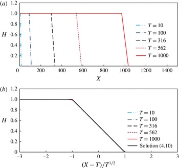
This solution agrees well with the numerical solution of the full equation (4.6) in the late time period, when the fluid–fluid interface contacts both the top and the bottom boundaries, as shown in figure 6. It should also be noted that as
 $T\rightarrow \infty$
,
 $X=T$
provides a leading-order approximation for the locations of the propagating fronts that attach to both the top and the bottom boundaries. In addition, since solution (4.10) requires the interface to attach to both boundaries, we need
 $X_{f2}(T)=T-T^{1/2}>0$
. Thus, we obtain a time scale beyond which the solution in (4.10) provides a good approximation:
 $T\geqslant \text{ord}(1)$
.
Time evolution of the fluid–fluid interface with
 $M=1$
in the late time period. (a) The interface has a linear structure at the front, but the slope of the front decreases in time. (b) The interface shapes at different times collapse in the new coordinate system. The analytical solution (4.10) is also plotted in (b), showing that it agrees very well with the numerical solutions.

5. Transition process between the early time and late time behaviours
We now show the transition processes between the various asymptotic approximations. We start by studying the time evolution of the shape of the fluid–fluid interface, then we study the propagation laws for the moving fronts at the top and the bottom boundaries.
5.1. The shape of the fluid–fluid interface
In order to effectively compare the shape of the fluid–fluid interface, we use different characteristic scales to rescale the horizontal and vertical coordinates. In particular, we use two possible length scales to rescale the horizontal coordinate, depending on the physical situation: either the location of the moving front along the bottom boundary
 $x_{f1}(t)$
, or the difference between the locations of the two moving fronts
 $x_{f1}(t)-x_{f2}(t)$
. Similarly, we use two possible length scales to rescale the vertical coordinate: either the depth of the porous medium
 $h_{0}$
, or the location of the vertical tip
 $h_{f}(t)\equiv h(0,t)$
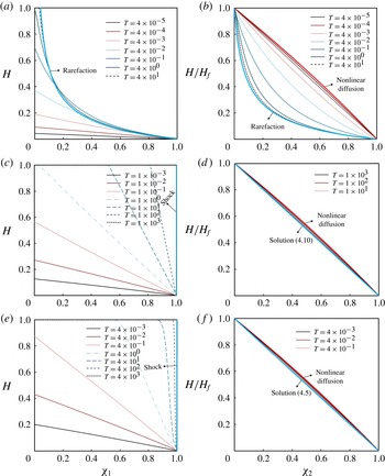
. The time evolution of the shape of the fluid–fluid interface is found from the numerical solutions of (2.12), and is shown in figure 7.
The time evolution of the fluid–fluid interface from the numerical solution of (2.12) compared to the late time asymptotic solutions. (a,b)
 $M=5$
: the injected fluid is more viscous than the displaced fluid. (c,d)
 $M=1$
: the injected and displaced fluids have equal viscosities. (e,f)
 $M=1/2$
: the injected fluid is less viscous than the displaced fluid. The solid curves represent the fluid–fluid interface before it contacts the top boundary, the dashed curves represent the interface after it contacts the top boundary, and the asymptotic solutions in these limits are also plotted in the figures. In (a,c,e) the horizontal coordinate is defined as
 ${\it\chi}_{1}\equiv x/x_{f1}(t)$
. In (b,d,f), the horizontal coordinate is defined as
 ${\it\chi}_{2}\equiv x/x_{f1}(t)$
before the interface attaches to the top boundary, and
 ${\it\chi}_{2}\equiv (x-x_{f2})/(x_{f1}-x_{f2})$
after the interface attaches to the top boundary.
 $H_{f}(T)\equiv h_{f}(t)/h_{0}$
is the location of the vertical tip, and by definition,
 $H_{f}(T)=1$
after the interface attaches to the top boundary.

We first rescale the horizontal coordinate by the location of the front at the bottom boundary, i.e. let
 ${\it\chi}_{1}\equiv x/x_{f1}(t)$
, and the vertical coordinate by the depth of the porous medium, i.e. let
 $H\equiv h/h_{0}$
. The time evolution of the fluid–fluid interface in this coordinate system is shown in figure 7(a,c,e), and compared with the late time asymptotic solutions. Figure 7(a) shows the time evolution of the moving interface for
 $M=5$
: the interface does not attach to the top boundary initially; then, the interface attaches to the top boundary and eventually approaches the prediction of the rarefaction wave solution (3.9). Figures 7(c) and 7(e) show the interface evolution for
 $M=1$
and
 $M=1/2$
: the interface propagates without attaching to the top boundary initially; then, the fluid–fluid interface attaches to the top boundary, and appears to approach the shape of the shock solution (3.12) as
 $T\rightarrow \infty$
. Note that in the late time period, the shock solution (3.12) provides a heuristic approximation to both solution (4.10) when
 $M=1$
and solution (4.5) when
 $M<1$
.
We next focus on the front structure of the fluid–fluid interface, as shown in figure 7(b,d,f). Before the interface attaches to the top boundary, the horizontal coordinate is defined as
 ${\it\chi}_{2}\equiv x/x_{f1}(t)$
with
 $x_{f1}(t)$
denoting the location of the front at the bottom boundary, while the vertical coordinate is
 $H/H_{f}$
with
 $H_{f}(T)\equiv h_{f}(t)/h_{0}$
denoting the dimensionless location of the vertical tip (recall figure 1
a). Once the interface attaches to both the top and bottom boundaries, we only focus on the region between the slower front
 $x_{2f}(t)$
at the top boundary, and the faster front
 $x_{1f}(t)$
at the bottom boundary; then the horizontal coordinate is defined as
 ${\it\chi}_{2}\equiv (x-x_{f2})/(x_{f1}-x_{f2})$
. Figure 7(b) demonstrates the time evolution of the interface for
 $M=5$
: in the early time period, the interface is similar to the shape of the self-similar solution to the nonlinear diffusion system (3.1) and (3.2); then, the solution departs from the early time approximation, and approaches the late time rarefaction wave solution (3.9). Figure 7(d) shows the evolution of the interface for
 $M=1$
: in the early time period, the shape is also similar to the shape of the self-similar solution to the nonlinear diffusion system (3.1) and (3.2); then the interface approaches the shape of the late time self-similar solution (4.10). Figure 7(f) demonstrates the evolution of the interface for
 $M=1/2$
: the interface is again similar in shape to the self-similar solution to (3.1) and (3.2) in the early time period; then the interface approaches the shape of the late time self-similar solution (4.5).
5.2. The propagation law
In our numerical simulations, we can track the moving fronts along the top and bottom boundaries in order to verify the propagation laws in the asymptotic limits, and study the transition processes between the individual regimes. From the theoretical discussion in § 3.1, in the early time period, the fluid–fluid interface can be approximated by a self-similar solution to the nonlinear diffusion equation (3.1) subject to (3.2), and the front along the bottom boundary propagates as
 $$\begin{eqnarray}X_{f1}(T)\approx 1.48T^{2/3},\end{eqnarray}$$
independent of the value of
 $M$
. In contrast, in §§ 4.1–4.2, we have shown that, in the late time period, the fluid–fluid interface propagates as a travelling wave solution (4.5) for
 $M<1$
, a self-similar solution (4.10) for
 $M=1$
, and a rarefaction wave solution (3.9) for
 $M>1$
. Thus, the moving front along the bottom boundary propagates according to
 $$\begin{eqnarray}X_{f1}(T)=\left\{\begin{array}{@{}ll@{}}T-1/(2(M-1)),\quad & M<1,\\ T+T^{1/2},\quad & M=1,\\ MT,\quad & M>1,\end{array}\right.\end{eqnarray}$$
while the moving front along the top boundary propagates according to
 $$\begin{eqnarray}X_{f2}(T)=\left\{\begin{array}{@{}ll@{}}T+1/(2(M-1)),\quad & M<1,\\ T-T^{1/2},\quad & M=1,\\ T/M,\quad & M>1.\end{array}\right.\end{eqnarray}$$
Again, note that the shock solution (3.12) predicts that
 $$\begin{eqnarray}X_{f1}(T)=X_{f2}(T)=T;\end{eqnarray}$$
(5.4) also provides a good approximation for the moving fronts of solution (4.5) when
 $M<1$
and solution (4.10) when
 $M=1$
, as
 $T\rightarrow \infty$
.
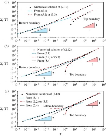
Now, we compare the numerical solutions of (2.12) and the analytical approximations in the early and late time regimes. As shown in figure 8(a), when
 $M>1$
, in the early time period, the propagation of the front along the bottom boundary obeys the
 $T^{2/3}$
power law for unconfined gravitational spreading. In the late time period, both the top and bottom fronts propagate at constant but distinct speeds, which agrees with the rarefaction wave solution (3.9), plotted as the dash-dotted lines. The transition process between the two asymptotes is captured by the numerical solutions at intermediate times.
The propagation laws for the front along the bottom boundary
 $X_{f1}(T)$
and the front along the top boundary
 $X_{f2}(T)$
: (a)
 $M=5$
; (b)
 $M=1$
; and (c)
 $M=1/2$
. (a) For
 $M=5$
, the propagation of the front exhibits a transition from the early time self-similar solution to the nonlinear diffusion problem (3.1) to the late time rarefaction wave solution (3.9). (b) For
 $M=1$
, the propagation of the front exhibits a transition from the early time self-similar solution to (3.1) to the late time self-similar solution (4.10). (c) For
 $M=1/2$
, the propagation of the front exhibits a transition from the early time self-similar solution to (3.1) to the late time travelling wave solution (4.5). The shock solution (3.12) is also plotted in (b,c) as a good approximation to both solution (4.10) and solution (4.5) in the late time period. The triangles represent numerical solutions of (2.12) at various times; the dashed and dash-dotted curves represent the moving fronts of the analytical early and late time asymptotic solutions, respectively.

For
 $M=1$
, the propagation of the bottom front also obeys a
 $T^{2/3}$
power law in the early time period, shown as the long-dashed line in figure 8(b); in the late time period, both the top and bottom fronts obey the predictions of the self-similar solution (4.10), plotted as the dash-dotted curves.
For
 $M<1$
, the propagation of the bottom front again obeys a
 $T^{2/3}$
power law in the early time period, which is the nonlinear diffusion behaviour, shown as the long-dashed line in figure 8(c); in the late time period, the solution (4.5) is also plotted as the dash-dotted curves, which agrees with the numerical solutions. The heuristic shock front location
 $X_{s}(T)=T$
is also plotted as the short-dashed line. The transition process is captured by numerical solutions at various intermediate times.
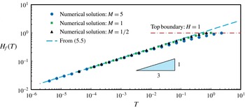
We can also track the vertical tip of the fluid–fluid interface. The locations of the vertical tip
 $H_{f}(T)\equiv H(0,T)$
, for
 $M=5$
,
 $M=1$
and
 $M=1/2$
, are shown in figure 9. In the early time period, the propagation of the vertical tip obeys
 $$\begin{eqnarray}H_{f}(T)\approx 1.30T^{1/3},\end{eqnarray}$$
independent of the value of
 $M$
, which is the prediction from the self-similar solution to the nonlinear diffusion system (3.3). On the other hand, for
 $M=5$
, the numerical solution deviates from the theoretical prediction at an earlier time. This behaviour is explained from the scaling argument at the end of § 3.1, where we estimate the early time period as
 $M^{-1}(T^{-1/3}-1)\geqslant \text{ord}({\it\epsilon}^{-1})$
. The vertical tip continues to grow until the fluid–fluid interface contacts the top boundary (
 $H=1$
).
The propagation law for the vertical tip
 $H_{f}(T)$
for
 $M=5$
,
 $M=1$
and
 $M=1/2$
. In the early time period, the growth of the vertical tip obeys a
 $T^{1/3}$
law, i.e. (5.5), which is the prediction of the self-similar solution to the nonlinear diffusion equation (3.1) subject to (3.2). In the late time period, the interface attaches to the top boundary
 $H=1$
, and the vertical tip no longer exists.

6. Flow regimes for fluid injection into a confined porous medium
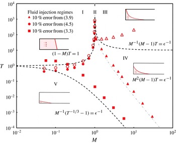
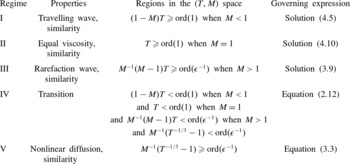
The behaviour of the fluid–fluid interface can be described by identifying flow regimes for point source injection into a confined porous medium, as shown in figure 10 and summarized in table 2. Five distinct dynamical regimes are identified, depending on two dimensionless groups:
 $M$
, the viscosity ratio of the displaced fluid to the injected fluid, and
 $T$
, the dimensionless time defined in (2.11). The diagram is best interpreted by imagining moving along a vertical line, from bottom to top, which corresponds to increasing time; then, the progression along
 $T$
includes regions where different analytical approximations apply.
Flow regimes for fluid injection into a confined porous medium. Five distinct dynamical regimes are identified, depending on two dimensionless groups:
 $M$
, the viscosity ratio of the displaced fluid to the injected fluid, and
 $T$
, the dimensionless time defined in (2.11). We have chosen
 ${\it\epsilon}=0.1$
in this plot except for
 $M^{-1}(T^{-1/3}-1)={\it\epsilon}^{-1}$
, where we have taken
 ${\it\epsilon}=0.3$
. In regime I, a travelling wave solution (4.5) is obtained as an approximation to the time evolution of the fluid–fluid interface. In regime II, the governing equation is reduced to (4.6), and a self-similar solution (4.10) is obtained for the full equation (2.12). In regime III, the governing equation is approximated by the hyperbolic equation (3.6), and a rarefaction wave solution (3.9) is obtained. In regime V, the governing equation is reduced to the nonlinear diffusion system (3.1) and (3.2), and a self-similar solution is found. Regime IV is the transition regime, and numerical simulation of the full governing equation (2.12) is necessary to describe the time evolution of the fluid–fluid interface. The dash-dotted line within regime IV represents the time when the rarefaction solution (3.9) starts to become a leading-order approximation for the interface at the bottom boundary. The symbols come from a comparison between self-similar solutions and numerical solutions, when the predictions for the front locations have a 10 % difference. The open and filled symbols correspond to the error for the top and bottom front locations, respectively. The dashed curves are estimates for the regime boundaries found by analysing the governing equations without considering the transition period for a self-similar solution to fully develop.

Flow regimes for fluid injection into a confined porous medium in a two-dimensional configuration with point source injection. Five distinct dynamical regimes are identified: a travelling wave regime (I), an equal-viscosity regime (II), a rarefaction regime (III), a transition regime (IV) and a nonlinear diffusion regime (V). The regimes in (
 $T,M$
) space in this table are estimated by analysing the governing equations without considering the transition period for a self-similar solution to fully develop.

There are four regimes representing the different asymptotic limits: regime I, a travelling wave regime with solution (4.5); regime II, an equal-viscosity regime with solution (4.10); regime III, a rarefaction regime with solution (3.9); and regime V, a nonlinear diffusion regime with a self-similar solution to (3.1) and (3.2). In addition, regime IV represents the transition between the early and late time asymptotic behaviours. The boundaries of the individual regimes have also been estimated by analysing the governing equations without considering the transition period to develop a self-similar solution as follows.
-
(i)
$M=1$
: in the late time period, a travelling wave solution (4.5) is obtained for
$M<1$
; a self-similar solution (4.10) is obtained for
$M=1$
; and a rarefaction solution (3.9) is obtained for
$M>1$
. In the transition regime,
$M$
will influence the profile shape of the fluid–fluid interface. In the early time period, the self-similar solution to the nonlinear diffusion system (3.1) and (3.2) is independent of
$M$
. -
(ii)
$M^{-1}(T^{-1/3}-1)=\text{ord}({\it\epsilon}^{-1})$
: earlier than this time scale, the buoyancy force provides the pressure gradient for the fluid motion, and the influence of injection is negligible. Equation (2.12) is reduced to the parabolic limit, i.e. the nonlinear diffusion system (3.1) and (3.2). A well-known self-similar solution is obtained for the time evolution of the fluid–fluid interface in this early time period. -
(iii)
$(1-M)T=\text{ord}(1)$
with
$M<1$
: beyond this time scale, the fluid–fluid interface attaches to both the top and bottom boundaries, and a travelling wave solution (4.5) is obtained to describe the dynamics of the interface. -
(iv)
$T=\text{ord}(1)$
with
$M=1$
: beyond this time scale, a self-similar solution (4.10) is found to describe the time evolution of the fluid–fluid interface, which attaches to both the top and bottom boundaries. -
(v)
$M^{-1}(M-1)T=\text{ord}({\it\epsilon}^{-1})$
with
$M>1$
: beyond this time scale, the dynamics of the interface can be described by a rarefaction solution (3.9).








Finally, in figure 10, we have plotted
 $M^{2}(M-1)T=\text{ord}({\it\epsilon}^{-1})$
, as the dash-dotted line within the transition regime IV. When
 $M>1$
, the rarefaction solution (3.9) becomes a good approximation to the front motion at the bottom boundary when
 $M^{2}(M-1)T\geqslant ~\text{ord}({\it\epsilon}^{-1})$
; the rarefaction solution (3.9) also becomes a good approximation at the top boundary when
 $T/M\geqslant \text{ord}({\it\epsilon}^{-1})$
and
 $M^{-1}(M-1)T\geqslant \text{ord}({\it\epsilon}^{-1})$
.
We have also conducted numerical simulations to verify the estimates based on analysing the equations without considering the time to fully develop the self-similar solutions from an initial condition. We have shown a comparison between numerical and self-similar solutions in figure 10. The filled and open symbols correspond to the times when the top and bottom front locations, respectively, have a 10 % difference between the predictions of the numerical and self-similar solutions; Pegler et al. (Reference Pegler, Huppert and Neufeld2014, figure 5) show a similar figure though only provide a priori estimates. Our numerical estimates appear to be more accurate than the estimates of Pegler et al. (Reference Pegler, Huppert and Neufeld2014), for example, in capturing the singular behaviour near
 $M=1$
in the late time period. In general, the a priori estimates without considering the transition period to fully develop the self-similar solutions appear to qualitatively provide the regime boundaries, while they do not necessarily provide accurate transition time scales especially for the top front locations when
 $M>1$
.
7. Summary and discussion
7.1. Summary
In this paper, we studied theoretically and numerically the problem of fluid injection into a confined porous medium in a two-dimensional configuration with point source injection. The evolution of the fluid–fluid interface was shown to be described by a nonlinear convection–diffusion equation (2.12). We considered the governing equation in different limits, and identified five distinct dynamical regimes for the fluid injection problem: a nonlinear diffusion regime, a transition regime, a travelling wave regime, an equal-viscosity regime, and a rarefaction regime, depending on two dimensionless groups: the viscosity ratio
 $M$
and the dimensionless time
 $T$
. The transition processes between the early and late time asymptotic limits were demonstrated by direct numerical simulations of the convection–diffusion equation (2.12) with appropriate boundary and initial conditions. Our study also provides connections between previous studies on fluid injection and propagation in porous media (e.g. Huppert & Woods Reference Huppert and Woods1995; Nordbotten & Celia Reference Nordbotten and Celia2006; Verdon & Woods Reference Verdon and Woods2007) by showing that these are either different limits of the nonlinear convection–diffusion equation, or transition solutions between the individual regimes. The regime diagram (figure 10; see also table 2) identifies the validity of the approximate analytical solutions, and provides a useful physical characterization of the fluid injection processes, spanning a range of time scales.
7.2. On a recent paper by Pegler et al. (Reference Pegler, Huppert and Neufeld2014)
As mentioned in the introduction, we learned about the recent publication by Pegler et al. (Reference Pegler, Huppert and Neufeld2014) on the same problem while we were finalizing our paper for submission. Our paper arrives at the same analytical solutions in the early time and late time regimes. However, in our study, we also emphasize the transition processes between the early time and late time behaviours, and we present more detailed numerical results for the evolving shape of the current during the transition process. In addition, we provide theoretical discussions on the time scales over which the transitions take place, and why the approximate analytical solutions may fail to capture the dynamics of the moving interface in these cases. The regime diagram (figure 10) provides more complete information for understanding the transition processes from the early time to the late time behaviours.
An experimental study is also conducted in a vertical Hele-Shaw channel filled with glass beads in Pegler et al. (Reference Pegler, Huppert and Neufeld2014). Experimental measurements of the interface shapes and front locations are obtained and compared with the theoretical predictions.
7.3. On the rarefaction wave solution
When
 $M>1$
, the injected fluid is less viscous than the displaced fluid. In this case, a rarefaction wave solution (3.9) is found for the hyperbolic equation (3.6) to describe the time evolution of the fluid–fluid interface in the late time period. In this limit, buoyancy no longer provides the pressure gradient to drive the fluid motion for the majority of the current; instead, the pressure gradient is provided by injection. It should be noted that
 $M>1$
corresponds to the situation when the viscous fingering phenomenon is expected to occur, and the classical Saffman–Taylor instability plays a key role in the propagation of the fluid–fluid interface (see e.g. Saffman & Taylor Reference Saffman and Taylor1958; Homsy Reference Homsy1987; Lenormand, Touboul & Zarcone Reference Lenormand, Touboul and Zarcone1988; Yortsos & Salin Reference Yortsos and Salin2006).
The rarefaction wave solution we obtained in the regime diagram is derived based on a one-dimensional model with a monotonic interface profile, assuming that fluid mixing and surface tension effects are negligible. The experimental results in a vertical Hele-Shaw channel packed with small glass beads (Pegler et al. Reference Pegler, Huppert and Neufeld2014) show that for the majority of the current away from the horizontal boundaries the rarefaction wave solution provides good approximations for the location of the moving fronts and the shape of the fluid–fluid interface. In the experiments of Pegler et al. (Reference Pegler, Huppert and Neufeld2014), the viscous fingering instability is suppressed at the reservoir scale, which may be due to the vertical pressure gradient from the hydrostatic pressure distribution (Pegler et al. Reference Pegler, Huppert and Neufeld2014).
7.4. On the extraction of the displaced fluid
In the model, we assumed that the densities of both the injected and the displaced fluids remain constant, i.e. the fluids are immiscible and the flow is incompressible. Thus, for a porous reservoir initially saturated with one fluid, the extraction of this fluid is required for the injection of another fluid. This requirement implies that certain fluid extraction or drainage mechanisms are associated with the porous reservoir (e.g. Acton, Huppert & Worster Reference Acton, Huppert and Worster2001; Pritchard Reference Pritchard2007; Neufeld et al. Reference Neufeld, Vella, Huppert and Lister2011; Zheng et al. Reference Zheng, Soh, Huppert and Stone2013). In practice, extraction of the displaced fluid can be realized, for example, by the presence of production or leaky wells downstream in the reservoir (e.g. Gasda, Bachu & Celia Reference Gasda, Bachu and Celia2004).
7.5. On the axisymmetric case
In this study, we considered the problem of fluid injection into a confined two-dimensional porous medium in Cartesian coordinates. Similar analyses can also be conducted for the fluid injection problem in axisymmetric coordinates. It should be noted that in Cartesian coordinates, in the unconfined regime, the vertical tip
 $h_{f}(t)$
for constant fluid injection increases with time as
 $h_{f}(t)\propto t^{1/3}$
at late times; however, this behaviour is different from the case in axisymmetic coordinates (see e.g. Lyle et al.
Reference Lyle, Huppert, Hallworth, Bickle and Chadwick2005; Nordbotten & Celia Reference Nordbotten and Celia2006). Detailed analysis of the axisymmetric fluid injection problem will be discussed in a forthcoming paper.
Acknowledgements
We thank the Princeton Carbon Mitigation Initiative for support of this research. We acknowledge the anonymous reviewers for helpful comments. We also thank T. Al-Housseiny, H. Huppert, C. Li, O. Pak, R. Socolow, and P. Tsai for helpful conversations. I.C.C. was supported by the National Science Foundation (NSF) under grant no. DMS-1104047 (at Princeton University) and by the LANL/LDRD Program through a Feynman Distinguished Fellowship (at Los Alamos National Laboratory). LANL is operated by Los Alamos National Security, LLC for the National Nuclear Security Administration of the US Department of Energy under contract no. DE-AC52-06NA25396.
Appendix A. Numerical scheme
A.1. Preliminaries, boundary and initial conditions
Instead of simulating the moving boundary problem on
 $(0,X_{f1}(T))$
, we solve (2.12) numerically on a fixed domain
 $(0,L)$
with appropriate boundary conditions at
 $X=0$
and
 $X=L$
. We assume that the fluid injection begins at
 $T=0$
, and before the point source injection there is only displaced fluid in the porous medium, so the initial condition is
 $$\begin{eqnarray}H(X,0)=0.\end{eqnarray}$$
In order to find the appropriate boundary conditions, we start by noting that
 $H(X,T)=0$
ahead of the front, i.e.
 $X\geqslant X_{f1}(T)$
; thus, the boundary condition at
 $X=L$
is given by
 $$\begin{eqnarray}H(L,T)=0.\end{eqnarray}$$
We can also integrate (2.12) from
 $X=0$
to
 $X=L$
, which gives
 $$\begin{eqnarray}\frac{\text{d}}{\text{d}T}\int _{0}^{L}H\text{d}X+\left[\frac{MH}{(M-1)H+1}-\frac{H(1-H)}{(M-1)H+1}\frac{\partial H}{\partial X}\right]_{0}^{L}=0.\end{eqnarray}$$
The condition of constant fluid injection requires that
 $\int _{0}^{L}H\text{d}X=T$
. Using (A 2) and
 $\lim _{X\rightarrow L}H(\partial H/\partial X)=0$
, (A 3) can be rewritten as
 $$\begin{eqnarray}\left.\left[\frac{MH}{(M-1)H+1}-\frac{H(1-H)}{(M-1)H+1}\frac{\partial H}{\partial X}\right]\right|_{X=0}=1,\end{eqnarray}$$
which is used as the boundary condition at
 $X=0$
. Equations (A 1), (A 2) and (A 4) provide the boundary and initial conditions for the numerical study.
A.2. The finite-difference scheme
Denoting
 $H_{X}\equiv \partial H/\partial X$
, the nonlinear convective flux
 $F(H)$
and diffusive flux
 $Q(H,H_{X})$
are defined as
 $$\begin{eqnarray}F(H)\equiv \frac{MH}{(M-1)H+1},\quad Q\left(H,H_{X}\right)\equiv \frac{H(1-H)}{(M-1)H+1}\frac{\partial H}{\partial X}.\end{eqnarray}$$
The conservative semi-discrete form of (2.12) is
 $$\begin{eqnarray}\frac{\text{d}H_{j}}{\text{d}T}=-\frac{R_{j+1/2}(T)-R_{j-1/2}(T)}{{\rm\Delta}X}+\frac{P_{j+1/2}(T)-P_{j-1/2}(T)}{{\rm\Delta}X},\end{eqnarray}$$
where
 $R_{j\pm 1/2}(T)$
denotes the discretized convective flux and
 $P_{j\pm 1/2}(T)$
denotes the discretized diffusive flux.
Following Kurganov & Tadmor (Reference Kurganov and Tadmor2000), the flux
 $R_{j+1/2}(T)$
is given by a second-order central discretization:
 $$\begin{eqnarray}R_{j+1/2}(T)\equiv \frac{F\left(H_{j+1/2}^{+}(T)\right)+F\left(H_{j+1/2}^{-}(T)\right)}{2}-\frac{a_{j+1/2}(T)}{2}\left[H_{j+1/2}^{+}(T)-H_{j+1/2}^{-}(T)\right],\end{eqnarray}$$
where the intermediate values
 $H_{j+1/2}^{\pm }(T)$
are given by
 $$\begin{eqnarray}H_{j+1/2}^{+}(T)\equiv H_{j+1}(T)-\frac{{\rm\Delta}X}{2}(H_{X})_{j+1}(T),\quad H_{j+1/2}^{-}(T)\equiv H_{j}(T)+\frac{{\rm\Delta}X}{2}(H_{X})_{j}(T),\end{eqnarray}$$
with the approximate derivative given by
 $$\begin{eqnarray}(H_{X})_{j}(T)\equiv \text{minmod}\left({\it\theta}\frac{H_{j}(T)-H_{j-1}(T)}{{\rm\Delta}X},\frac{H_{j+1}(T)-H_{j-1}(T)}{2{\rm\Delta}X},{\it\theta}\frac{H_{j+1}(T)-H_{j}(T)}{{\rm\Delta}X}\right),\end{eqnarray}$$
where
 $1\leqslant {\it\theta}\leqslant 2$
, and we choose
 ${\it\theta}=1$
in this study. The ‘minmod’ limiter is used following Kurganov & Tadmor (Reference Kurganov and Tadmor2000). The local propagation speed for a convex flux is given by
 $$\begin{eqnarray}a_{j+1/2}(T)=\max \left[\left|\frac{\text{d}F}{\text{d}H}\left(H_{j+1/2}^{-}(T)\right)\right|,\left|\frac{\text{d}F}{\text{d}H}\left(H_{j+1/2}^{+}(T)\right)\right|\right].\end{eqnarray}$$
In addition, the discretized diffusive flux
 $P_{j+1/2}(T)$
is given by a central difference approximation, which is second-order accurate:
 $$\begin{eqnarray}P_{j+1/2}(T)=\frac{1}{2}\left[Q\left(H_{j}(T),\frac{H_{j+1}(T)-H_{j}(T)}{{\rm\Delta}X}\right)+Q\left(H_{j+1}(T),\frac{H_{j+1}(T)-H_{j}(T)}{{\rm\Delta}X}\right)\right].\end{eqnarray}$$
Finally, we used a second-order Runge–Kutta method for the time-stepping of (A 6). Thus, the scheme is formally second-order accurate in both time and space. This central scheme treats the smooth and non-smooth regions separately, which leads to small numerical viscosity on the order of
 $O(({\rm\Delta}X)^{3})$
, independent of
 $O(1/{\rm\Delta}T)$
. The scheme is able to capture the shocks and rarefactions with high resolution.
Appendix B. An estimate of the early time period
In this section, we provide a more formal discussion on the estimate of the early time period based on analysing the governing equations. Since the time scales of the propagation may vary by orders of magnitude, we first rewrite the dimensionless time
 $T$
, defined in (2.11), as
 $T=\mathscr{T}{\it\epsilon}^{-n}$
, where
 $\mathscr{T}=\text{ord}(1)$
, and
 ${\it\epsilon}\ll 1$
. The notation
 $\text{ord}(1)$
denotes terms strictly of order unity (Hinch Reference Hinch1991). Thus, different values of
 $n$
represent different time scales. For example,
 $n<0$
represents the time period when
 $T<\text{ord}(1)$
,
 $n=0$
represents the intermediate time when
 $T=\text{ord}(1)$
, and
 $n>0$
represents the time period when
 $T>\text{ord}(1)$
. Note that
 ${<}$
and
 ${>}$
signs with regard to
 $\text{ord}(\cdot )$
are used in the sense of Hinch (Reference Hinch1991). We can use either
 $T$
or
 $n$
to represent time.
In addition, the value of
 $M$
can vary by orders of magnitude for real problems, depending on the viscosity of the invading and displaced fluids. We write
 $M$
as
 $M=\mathscr{M}{\it\epsilon}^{-m}$
, where
 $\mathscr{M}=\text{ord}(1)$
. As a result, different values of
 $m$
represent different viscosity ratios:
 $m<0$
represents the situation when
 $M<\text{ord}(1)$
,
 $m=0$
represents the situation when
 $M=\text{ord}(1)$
, and
 $m>0$
represents the situation when
 $M>\text{ord}(1)$
. We may use either
 $M$
or
 $m$
to represent the viscosity ratio of the fluids.
As mentioned in § 3, the form of the governing equation (2.12) suggests that when
 $T=\text{ord}(1)$
, the convective and the diffusive terms have the same order of magnitude. However, as hinted by the numerical results in § 2.4, in the early time period the diffusive term is dominant, while in the late time period the convective term is dominant. To look for the possible asymptotic behaviours in the early and the late time periods, we can rescale (2.6), using different characteristic time and length scales.
The flow is unconfined in the early time period, when the fluid–fluid interface only touches the bottom boundary. Thus,
 $h_{0}$
is not an appropriate characteristic scale for the height
 $h(x,t)$
. In fact, there are no fixed characteristic length and time scales for such a moving boundary problem.
When
 $M<\text{ord}(1)$
, i.e.
 $m<0$
, we define dimensionless variables
 $T_{1}$
,
 $H_{1}$
and
 $X_{1}$
using characteristic scales
 $t_{c}$
,
 $h_{c}$
and
 $x_{c}$
. Then, (2.6) becomes
 $$\begin{eqnarray}\frac{\partial H_{1}}{\partial T_{1}}=\frac{\partial }{\partial X_{1}}\left[\frac{H_{1}\left(1-H_{1}\right)}{\left(\mathscr{M}{\it\epsilon}^{-m}-1\right)H_{1}+1}\frac{\partial H_{1}}{\partial X_{1}}\right]+O({\it\epsilon}^{-m}).\end{eqnarray}$$
In this case, the leading-order form of (B 1) is a nonlinear diffusion equation:
 $$\begin{eqnarray}\frac{\partial H_{1}}{\partial T_{1}}=\frac{\partial }{\partial X_{1}}\left(H_{1}\frac{\partial H_{1}}{\partial X_{1}}\right),\end{eqnarray}$$
which was studied in § 3.1. When
 $M\geqslant \text{ord}(1)$
, i.e.
 $m\geqslant 0$
, on the other hand, we define dimensionless variables
 $T_{2}$
,
 $H_{2}$
and
 $X_{2}$
using new characteristic scales
 ${\it\epsilon}^{3(1+m)}t_{c}$
,
 ${\it\epsilon}^{(1+m)}h_{c}$
and
 ${\it\epsilon}^{2(1+m)}x_{c}$
. Then, (2.6) becomes
 $$\begin{eqnarray}\frac{\partial H_{2}}{\partial T_{2}}=\frac{\partial }{\partial X_{2}}\left[\frac{H_{2}(1-{\it\epsilon}^{(1+m)}H_{2})}{\left(\mathscr{M}{\it\epsilon}^{-m}-1\right){\it\epsilon}^{(1+m)}H_{2}+1}\frac{\partial H_{2}}{\partial X_{2}}\right]+O({\it\epsilon}).\end{eqnarray}$$
Note that
 $|{\it\epsilon}^{(1+m)}H_{2}|=O({\it\epsilon}^{(1+m)})$
and
 $|(\mathscr{M}{\it\epsilon}^{-m}-1){\it\epsilon}^{(1+m)}H_{2}|=O({\it\epsilon})$
when
 $m\geqslant 0$
. Again, in this case, the leading-order form of (B 3) is a nonlinear diffusion equation:
 $$\begin{eqnarray}\frac{\partial H_{2}}{\partial T_{2}}=\frac{\partial }{\partial X_{2}}\left(H_{2}\frac{\partial H_{2}}{\partial X_{2}}\right)\!.\end{eqnarray}$$
Thus, the early time period is estimated as
 $T\leqslant \text{ord}(1)$
and
 $TM^{3}\leqslant \text{ord}({\it\epsilon}^{3})$
, or equivalently,
 $n\leqslant \min (0,-3(1+m))$
in the
 $(n,m)$
space. The leading-order terms of (2.6) become a nonlinear diffusion equation, i.e. either (B 2) when
 $M<\text{ord}(1)~(m<0)$
, or (B 4) when
 $M\geqslant \text{ord}(1)~(m\geqslant 0)$
. Both (B 2) and (B 4) can be rewritten as (3.1) in the
 $(X,T)$
space. Note that this estimate is slightly different from the estimate at the end of § 3.1, i.e.
 $M^{-1}(T^{-1/3}-1)\geqslant \text{ord}({\it\epsilon}^{-1})$
. Both estimates are in a good agreement with numerical results.