1. Introduction
The calming effect of surface oil on oceanic waves was recognized by sponge and pearl divers as early as the time of Pliny the Elder. Franklin, Brownrigg & Farish (Reference Franklin, Brownrigg and Farish1774), citing Pliny’s account, also reported on sailors calming ocean waves with oil. Franklin et al. concluded from experiments that oil significantly damps short-wavelength small-amplitude waves, and conjectured that it would also induce damping of larger long-wavelength waves. Lord Kelvin (Thomson Reference Thomson1871) first identified short-wavelength capillary-driven waves and long-wavelength gravity-driven waves as two regimes within the same mathematical formulation. Kelvin’s famous dispersion relation describing the wavelength dependence of the speed of gravity–capillary waves shows a crossover from capillary to gravity waves at the minimum wave speed.
Much effort has since been devoted to studying the damping effect of surfactants on gravity–capillary waves (Reynolds Reference Reynolds1880; Levich Reference Levich1941; Dorrestein Reference Dorrestein1951; Goodrich Reference Goodrich1961; Lucassen-Reynders & Lucassen Reference Lucassen-Reynders and Lucassen1970). With or without a surfactant, energy is lost due to the viscosity of the fluid and the vorticity of the flow. By adding a surfactant, the surface can experience additional tangential stresses which, balanced by viscous stress in the bulk, increase the vorticity of the bulk flow. These tangential surface stresses are a consequence of the complex relation between surface stress and strain rate, which depends upon the bulk flow, surface velocity and surfactant density. The primary contribution to the tangential surface stress is the Marangoni effect (Behroozi et al. Reference Behroozi, Cordray, Griffin and Behroozi2007), in which the advection of the surfactant monolayer by the passing wave results in gradients in the surfactant density field, inducing surface tension gradients and vorticity in the bulk fluid flow. Thus, beyond quantifying the damping effect of surfactants on gravity–capillary waves, it is important also to understand the distribution of surfactant on the surface of the fluid. In this paper, we combine two experimental techniques to measure both the surface height and surfactant density fields. Using a physically motivated ansatz, we quantify both fields and measure parameters such as the complex wavenumber and phase. This provides a spatiotemporal description of the surfactant accumulation within the wave pattern.
Surface waves can be generated and sustained in a variety of ways, depending on how energy is injected into the fluid system. A vertically vibrated fluid will generate both travelling meniscus waves, excited by the contact line at the container wall, and standing Faraday waves, first observed by Faraday (Reference Faraday1831). When the driving acceleration
 $a(t)=a_{0}\sin ({\it\omega}t)$
is weak, only meniscus waves perturb the fluid surface. However, when
 $a_{0}$
is increased beyond a critical acceleration amplitude
 $a_{c}$
, so that the injection of energy exceeds the dissipation due to the bulk viscosity, the meniscus wave becomes unstable to Faraday waves, which grow to a finite amplitude (Benjamin & Ursell Reference Benjamin and Ursell1954; Chen & Viñals Reference Chen and Viñals1999). The parameter
 $a_{c}$
depends on the driving frequency
 ${\it\omega}$
, the container geometry, contact line dynamics and fluid properties (Benjamin & Scott Reference Benjamin and Scott1979; Douady Reference Douady1990; Edwards & Fauve Reference Edwards and Fauve1994; Bechhoefer et al.
Reference Bechhoefer, Ego, Manneville and Johnson1995; Chen & Viñals Reference Chen and Viñals1999). The emergent Faraday waves can be either harmonic (frequency
 ${\it\omega}$
) or subharmonic (frequency
 ${\it\omega}/2$
), while the meniscus waves are always harmonic.
Recently, there have been advances in our understanding of the relationship between the surface height field
 $h(\boldsymbol{r},t)$
of meniscus waves and its interaction with surfactant molecules adsorbed onto the surface, described by the density field
 ${\it\Gamma}(\boldsymbol{r},t)$
. The theory of surfactant-laden meniscus waves in a cylindrical geometry, developed by Bock (Reference Bock1991), Saylor, Szeri & Foulks (Reference Saylor, Szeri and Foulks2000) and Picard & Davoust (Reference Picard and Davoust2006), proceeds from the treatment of two-dimensional travelling gravity–capillary waves in a Cartesian geometry (Lucassen-Reynders & Lucassen Reference Lucassen-Reynders and Lucassen1970). In this theory, the fluid motion in the incompressible bulk is modelled with the linearized Navier–Stokes equations, and the vertical and horizontal displacements of the surface satisfy the surface stress and kinematic boundary conditions. Bock (Reference Bock1991) showed that, for a fluid of equilibrium height
 $h_{0}$
, the deviation in the surface height field
 ${\rm\Delta}h(\boldsymbol{r},t)=h(\boldsymbol{r},t)-h_{0}$
for inward- and outward-travelling cylindrical gravity–capillary waves follow Hankel modes of the first and second kinds. Recognizing that meniscus waves are a superposition of inward- and outward-travelling waves, Saylor et al. (Reference Saylor, Szeri and Foulks2000) found that meniscus waves follow a
 $\text{J}_{0}$
Bessel mode. Subsequently, Picard & Davoust (Reference Picard and Davoust2006) derived an expression for the deviation of the surfactant density field from an equilibrium density
 ${\it\Gamma}_{0}$
. The quantity
 ${\rm\Delta}{\it\Gamma}(\boldsymbol{r},t)={\it\Gamma}(\boldsymbol{r},t)-{\it\Gamma}_{0}$
also follows a
 $\text{J}_{0}$
Bessel mode, with the same wavenumber and damping factor as the surface height field. Because the motion of a fluid surface element is affected by gradients in the interfacial surface tension
 ${\it\sigma}({\it\Gamma})$
, the magnitude of the surface compression modulus
 ${\it\epsilon}={\it\Gamma}_{0}\text{d}{\it\sigma}/\text{d}{\it\Gamma}$
controls the phase shift between the
 ${\rm\Delta}h$
and
 ${\rm\Delta}{\it\Gamma}$
fields (Lucassen-Reynders & Lucassen Reference Lucassen-Reynders and Lucassen1970).
For Faraday waves, Kumar & Matar (Reference Kumar and Matar2002, Reference Kumar and Matar2004) used a linear stability analysis to determine the wave’s critical acceleration and wavelength, and predicted that the Faraday wave emerges with a spatial displacement (phase shift) between the fields
 ${\rm\Delta}h$
and
 ${\rm\Delta}{\it\Gamma}$
. Inspired by reports (Douady, Fauve & Thual Reference Douady, Fauve and Thual1989) of a rotating Faraday wave, Martín & Vega (Reference Martín and Vega2006) conjectured that the rotation was induced by the presence of a contaminant and showed that the drift can be generated when the reflection symmetry of the streaming flow breaks. Ubal, Giavedoni & Saita (Reference Ubal, Giavedoni and Saita2005) executed numerical simulations of the gravity-modulated Navier–Stokes equations and predicted that neither
 ${\rm\Delta}h$
nor
 ${\rm\Delta}{\it\Gamma}$
evolve sinusoidally in time. They found that
 ${\rm\Delta}h$
lags behind
 ${\rm\Delta}{\it\Gamma}$
, characterized as a temporal phase shift between the two fields.
Many experiments with surfactant-laden gravity–capillary waves have focused on quantifying energy dissipation through either direct or indirect measurements of the surface height field alone (Case & Parkinson Reference Case and Parkinson1957; Davies & Vose Reference Davies and Vose1965; Jiang, Chiew & Valentini Reference Jiang, Chiew and Valentini1993; Henderson & Miles Reference Henderson and Miles1994; Henderson Reference Henderson1998; Saylor et al.
Reference Saylor, Szeri and Foulks2000; Behroozi et al.
Reference Behroozi, Cordray, Griffin and Behroozi2007), and these works have demonstrated that the damping rate does not depend on whether the gravity–capillary waves are either standing or travelling. Despite this progress, a quantitative understanding of the spatiotemporal dynamics of
 ${\it\Gamma}(\boldsymbol{r},t)$
remains elusive. Previous measurements of
 ${\it\Gamma}$
have utilized surface potential measurements in a small region near an electric probe (Lange & Hühnerfuss Reference Lange and Hühnerfuss1984; Hühnerfuss, Lange & Walter Reference Hühnerfuss, Lange and Walter1985; Lange & Hühnerfuss Reference Lange and Hühnerfuss1986). These studies report a temporal phase shift between
 ${\rm\Delta}{\it\Gamma}$
and
 ${\rm\Delta}h$
, with the caveat that it is necessary to account for both the response time of the probes and the finite time for the wave to pass from the surface potential probe to the wave height probe (Lucassen-Reynders Reference Lucassen-Reynders1987). In this paper, we present novel methods for measuring the spatial and temporal dynamics of
 ${\rm\Delta}{\it\Gamma}$
and
 ${\rm\Delta}h$
, using stroboscopic imaging to avoid this complication. These methods allow us to quantify the accumulation of surfactant relative to the crests/troughs of the surface waves. In addition, we test the extent to which the spatiotemporal dynamics can be described by a superposition of solutions for the meniscus and Faraday waves.
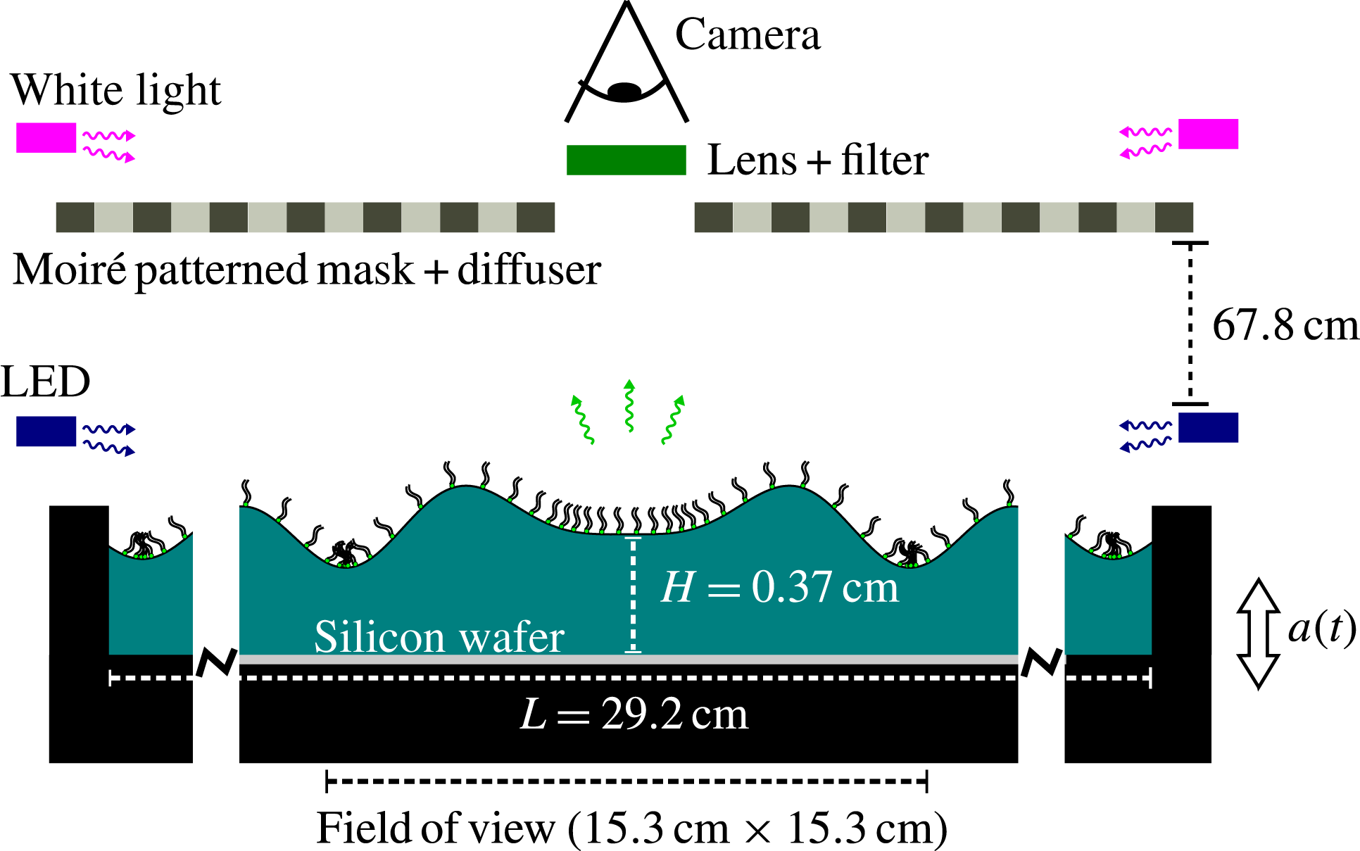
Our experimental apparatus, shown schematically in figure 1 and described in detail in § 2, consists of a shallow cylindrical container holding a thin layer of water covered with a monolayer of fluorescently tagged lipids. We drive the system with vertical oscillations just above onset for the Faraday instability and make stroboscopic measurements of both the surface height field
 $h(\boldsymbol{r},t)$
and the surfactant density field
 ${\it\Gamma}(\boldsymbol{r},t)$
. To obtain
 $h$
, we illuminate the fluid with a target pattern, and use a combination of ray tracing and nonlinear fitting to invert the resulting moiré image. For
 ${\it\Gamma}$
, we phase-average the fluorescence intensity from the tagged molecules using images acquired stroboscopically over many cycles of the driving oscillation, and convert these to quantitative measurements of the surfactant density field. A key advantage of these techniques is that they are non-invasive. Additionally, this and similar optical techniques (Vogel et al.
Reference Vogel, Hirsa, Kelley and Korenowski2001; Fallest et al.
Reference Fallest, Lichtenberger, Fox and Daniels2010; Strickland et al.
Reference Strickland, Hin, Sayanagi, Gaebler, Daniels and Levy2014; Swanson et al.
Reference Swanson, Strickland, Shearer and Daniels2014) for measuring
 ${\it\Gamma}$
depend upon the mean distance between the fluorophores and therefore are not affected by the dynamics of either molecular rearrangement or domain formation/relaxation.
Experimental apparatus. The container (black) is connected by low-friction air bushings to an electromagnetic shaker, and filled with a thin layer of water onto which a monolayer of NBD-PC surfactant is deposited. The shaker vibrates the container vertically with acceleration
 $a(t)=a_{0}\sin {\it\omega}t$
, generating meniscus and Faraday waves. The fluorescence imaging system involves a ring of blue LEDs around the outer edge that excites the fluorophore on the lipids; digital images of the fluorescence emission are collected through an optical notch filter. A silicon wafer sits flush with the bottom surface of the container, and reflects the excess light from the LEDs away from the camera. The moiré imaging system consists of a patterned light source shining downwards on the fluid surface, and the camera that records the distorted reflection of the pattern.

In § 3, we show that our data are well approximated by a linear superposition of a standing Faraday wave mode and a travelling meniscus wave mode. We decompose the data into these two separate components in order to examine the spatiotemporal dynamics of each. We determine that the surfactant accumulates on the leading edge of the meniscus waves and in the troughs of the Faraday waves. The meniscus waves are represented by
 $\text{J}_{0}$
Bessel functions. The fields
 ${\rm\Delta}h$
and
 ${\rm\Delta}{\it\Gamma}$
have the same wavenumber within experimental error, but the damping factors for the two fields do not agree. Since the temporal phase shift between the two fields is measured to be as large as 2 rad, in excess of the theoretical maximum of
 ${\rm\pi}/2$
rad (Lucassen-Reynders & Lucassen Reference Lucassen-Reynders and Lucassen1970), we conjecture that longitudinal waves (Lucassen Reference Lucassen1968b
) may also be present. The Faraday waves are represented by
 $\text{J}_{n}$
Bessel functions. The fields
 ${\rm\Delta}h$
and
 ${\rm\Delta}{\it\Gamma}$
have the same symmetry number
 $n$
and the same wavenumber within experimental error. We observe that the whole Faraday wave pattern rotates around the centre of the pattern in the same direction as an observed spatial phase shift between
 ${\rm\Delta}h$
and
 ${\rm\Delta}{\it\Gamma}$
fields. Both fields evolve sinusoidally and are temporally phase shifted by roughly 2.4 rad.
In § 4, we discuss our observations about surfactant-covered meniscus and Faraday waves in the context of their respective theoretical frameworks. We also consider the possible presence of resonantly excited longitudinal waves in our system, which could account for the anomalously large temporal phase shifts and the disagreement in the damping factors. We highlight the suitability of using measurements of
 ${\rm\Delta}{\it\Gamma}$
and the temporal phase shift between
 ${\rm\Delta}h$
and
 ${\rm\Delta}{\it\Gamma}$
as a way to probe the interfacial rheology. Finally, we contrast the dynamics of these molecular monolayers with the dynamics of a monolayer of millimetric sized particles (Sanlı, Lohse & van der Meer Reference Sanlı, Lohse and van der Meer2014).
2. Experiment
We excite travelling meniscus waves and standing Faraday waves on a surfactant-covered fluid layer by subjecting the system to a vertical sinusoidal oscillation, shown schematically in figure 1. A mechanical driving system provides the vertical acceleration, and two quasi-independent imaging systems measure the response of both the surfactant and the fluid surface. The fluorescence imaging (FI) system directly measures the surfactant density field
 ${\it\Gamma}(\boldsymbol{r},t)$
(details provided in § 2.2), and the moiré imaging (MI) system indirectly measures the surface height field (§ 2.3). Finally, we use a physically motivated ansatz (§ 2.4) to support the ray tracing and image analysis in order to convert the MI data to a surface height field
 $h(\boldsymbol{r},t)$
and to quantify properties of the deviations of the surface height field
 ${\rm\Delta}h(\boldsymbol{r},t)=h(\boldsymbol{r},t)-h_{0}$
and surfactant density field
 ${\rm\Delta}{\it\Gamma}(\boldsymbol{r},t)={\it\Gamma}(\boldsymbol{r},t)-{\it\Gamma}_{0}$
.
We perform all experiments just above the onset of the Faraday instability in order to excite a stable (non-chaotic) surface mode. To reach this regime, we quasi-statically increase the driving acceleration in steps of
 $1.5\times 10^{-3}~\text{g}$
until the Faraday wave pattern is just identifiable in the moiré images. Each quasi-static step during this preparation stage lasts for 90 s, during which the driving acceleration is held constant. In the data-collection stage, the amplitude of the voltage signal for the electromagnetic shaker is held constant while we alternately collect MI and FI data. Although we collect data just above the Faraday wave onset, we nonetheless observe that the entire pattern rotates on the order of
 $10^{\circ }~\text{min}^{-1}$
. Similar rotations have been observed in other experiments, with the rotation axis slightly displaced from the centre of the container (Gollub & Meyer Reference Gollub and Meyer1983; Douady et al.
Reference Douady, Fauve and Thual1989). During image analysis, we remove the rotation by rotating images back to a common reference.
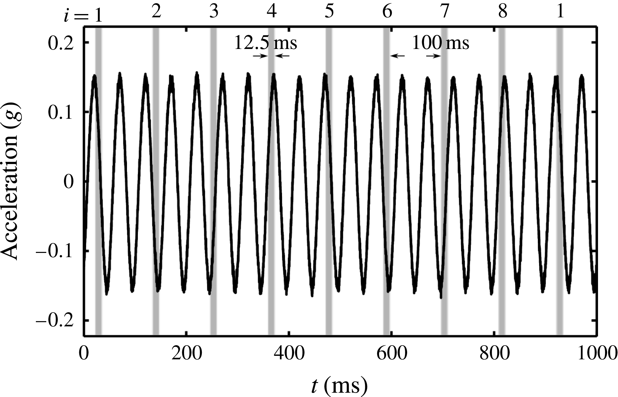
To increase the signal-to-noise ratio, all FI is performed stroboscopically to phase-average over the low-intensity signal. To measure subperiod dynamics, we set the exposure time for each image to be
 $1/8$
th of the subharmonic Faraday wave oscillation period (see figure 2 for a description). We then average 700 images taken at the same phase to obtain a set of eight composite images. By adding/subtracting pairs of these eight images, we can visualize any periodic pattern in the surfactant distribution that is
 $1\times$
,
 $1/2\times$
or
 $1/4\times$
the Faraday wave period. Finally, each of the eight phases are interpreted as surfactant concentration through a linear calibration. Through these means, we are able to probe average dynamics on time scales faster than a single oscillation. Obtaining this fluorescence composite data takes 14 min in total, during which time the Faraday wave rotates through roughly
 $140^{\circ }$
. We take a series of 32 moiré images during each minute of the data collection both to account for the rotation and to measure the surface height field. The additional use of an ansatz (§ 2.4) to fit the fluorescence composite data allows us to further characterize the observed fields via their amplitudes, wavenumbers, damping factors, phase shifts, etc.
Stroboscopic imaging allows for the collection and phase-averaging of low-intensity fluorescence images over many cycles. During each second of the experiment, the container oscillates 20 times with an acceleration
 $a(t)$
(black curve). During that second, the camera is triggered at four different phases of the oscillation (eight different phases of the Faraday wave oscillation). The eight distinct phases (represented as
 $i=1$
to
 $i=8$
) each have an exposure time of
 $1/8$
th of the Faraday wave period, represented by the width of the grey bars. The time from the end of one exposure to the beginning of the next exposure is one whole Faraday wave period (100 ms), so that we sequentially sample each of the eight phases cyclically. The same stroboscopic pattern was used for both experiments, and both the FI and MI data.

2.1. Apparatus and materials
In order to produce stable Faraday waves, we drive the system with a constant sinusoidal acceleration just above the onset acceleration. We use a PM50A MB Dynamics shaker (peak force 220 N) mounted on a vibration isolation table. The driving acceleration is transferred from the shaker to the container by two parallel shafts. Each shaft is guided by a low-friction air bushing, and the parallel placement of the two bushings suppresses rotational motion. The mounting bar for the container contains two two-axis ADXL203 accelerometers, sampled at a rate of 20 kHz with a noise threshold of approximately
 $10^{-3}~\text{g}$
. The power density spectra of the driving acceleration shows the 20 Hz driving to be greater than the higher harmonics by a factor of at least
 $10^{-3}$
.
To collect data near onset, we separate each experiment into two stages, a preparation stage wherein the amplitude of the sinusoidal acceleration is increased in small steps of
 $1.5\times 10^{-3}~\text{g}$
every 90 s, and a data-collection stage with constant driving. In the preparation stage, we use a proportional control to monitor the amplitude of the acceleration to within
 $5\times 10^{-4}~\text{g}$
. In the data-collection stage, we turn off the proportional control and keep the shaker driving voltage constant. In both experiments, we observed a small drift in the amplitude of the acceleration of roughly
 $5\times 10^{-3}~\text{g}$
during the data-collection stage.
The choice of materials in our experiments is guided by two important considerations: the sensitivity of surface experiments to preparation and handling, and the requirement of a low fluorescence background. The black-anodized container is made of aluminium machined into a cylindrical well of radius 14.6 cm and depth 0.52 cm. A 200 mm silicon wafer is embedded into the base of the well so that the wafer’s top surface is flush with the bottom of the well. The silicon wafer provides both a reproducible substrate and excellent reflectivity (Strickland et al. Reference Strickland, Hin, Sayanagi, Gaebler, Daniels and Levy2014).
Prior to each experiment, we clean the container with detergent and perform a final rinse with
 $18.2~\text{M}{\rm\Omega}$
water before drying with dry nitrogen gas. The silicon wafer is cleaned for 5 min in an oxygen plasma environment, and all glassware is cleaned by soaking for several hours in a 2 % Contrad 70 solution. These materials are rinsed with
 $18.2~\text{M}{\rm\Omega}$
water and dried with dry nitrogen gas immediately before the experiment. To initialize each experiment, we fill the container to a depth of
 $h_{0}=0.37\pm 0.02~\text{cm}$
(below the brim of the container) with
 $18.2~\text{M}{\rm\Omega}$
water. Using a micropipette, we deposit a solution of chloroform and NBD-PC (1-palmitoyl-2-{12-[(7-nitro-2-1,3-benzoxadiazol-4-yl)amino]dodecanoyl}-sn-glycero-3-phosphocholine from Avanti Polar Lipids) onto the clean water surface. The concentration of NBD-PC in solution is
 $1~\text{mg}~\text{ml}^{-1}$
, and, owing to the low interfacial tension between chloroform and water, the droplets spread over the fluid surface.
In this paper, we report on two experimental runs: experiment 1 with
 ${\it\Gamma}_{0}=0.3~{\rm\mu}\text{g}~\text{cm}^{-2}$
, and experiment 2 with
 ${\it\Gamma}_{0}=0.2~{\rm\mu}\text{g}~\text{cm}^{-2}$
. Both runs are below the critical monolayer concentration for NBD-PC on water, which is
 ${\it\Gamma}_{c}=0.35~{\rm\mu}\text{g}~\text{cm}^{-2}$
(Tsukanova, Grainger & Salesse Reference Tsukanova, Grainger and Salesse2002). The mean density
 ${\it\Gamma}_{0}$
is calculated from the deposited volume of chloroform solution and the known dimensions of the container. To reduce disturbance from external air currents and dust, the entire apparatus is enclosed in a plastic tent, and a combination hygro-thermometer is used to observe variations in the temperature and humidity within the tent. For experiment 1, the temperature and humidity were within the range
 $23.9\pm 0.4\,^{\circ }\text{C}$
and
 $18.5\pm 0.5$
%, respectively; while for experiment 2, they were
 $24.6\pm 0.4\,^{\circ }\text{C}$
and
 $18.0\pm 0.5$
%.
2.2. Fluorescence imaging
The FI technique is based on quantifying spatiotemporal deviations of the surfactant density field (
 ${\rm\Delta}{\it\Gamma}$
) from the mean density by observing the fluorescence intensity in digital images (Fallest et al.
Reference Fallest, Lichtenberger, Fox and Daniels2010; Strickland et al.
Reference Strickland, Hin, Sayanagi, Gaebler, Daniels and Levy2014; Swanson et al.
Reference Swanson, Strickland, Shearer and Daniels2014). The NBD-PC surfactant molecule contains a fluorophore with an excitation peak at 464 nm and an emission peak at 531 nm. Eight blue light-emitting diodes (LEDs) (1.5 W, 467 nm, from Visual Communications Company LLC) are mounted around the edge of the container to provide uniform excitation and illuminate the fluid surface at a low angle. The silicon wafer substrate reflects unabsorbed light away from the imaging system, thus minimizing the background noise. An Andor Luca-R camera fitted with a Newport
 $530\pm 10~\text{nm}$
bandpass filter is positioned above the centre of the experiment and takes images of surfactant fluorescence within a field of view of width 15.4 cm. Because the camera images its own reflection near the centre of the system, we report measurements for an annular region of the fluid surface.
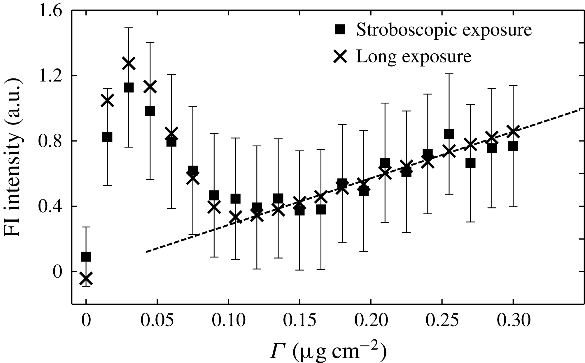
We calibrate the fluorescence intensity by performing experiments on a flat fluid surface covered with a known quantity of surfactant. In order to ensure a uniform density on the surface, we deposit the chloroform-dispersed surfactant onto the clean surface of water, wait 60 s for the chloroform to evaporate, and then drive the system at 20 Hz and
 $0.2~g$
(above the Faraday onset) for 60 s. This promotes redistribution of the surfactant, so that, after turning off the shaker and waiting for the fluid to settle back to its flat state, the surfactant is uniformly distributed (verified by a visual inspection of the calibration images). In this state, we collect two types of data: 700 images with the same exposure time as used for the FI composite images, and a final image with a single 2 s exposure time to provide a consistency check on the trend. The mean and standard error of the fluorescence intensity as a function of
 ${\it\Gamma}$
, reported in figure 3, are calculated from a composite of 700 images, as is done for each phase-averaged stroboscopically acquired image. We observe that the calibration is linear for
 ${\it\Gamma}>0.1~{\rm\mu}\text{g}~\text{cm}^{-2}$
. This corresponds to a regime in which the equation of state relating surfactant density and surface tension is also linear (Tsukanova et al.
Reference Tsukanova, Grainger and Salesse2002).
Calibration of surfactant fluorescence intensity as a function of surfactant density. The stroboscopic exposure data were obtained with the same exposure time, number of images and gain settings as used for the FI technique. The long-exposure data were obtained with a single 2 s exposure and no gain, to confirm the trend. The markers show the mean intensity of the pixels within the field of view, while the error bars illustrate the standard error of the pixels for the stroboscopic exposure data. The linear fit, shown as a dashed line, is used in the range
 ${\it\Gamma}>0.1~{\rm\mu}\text{g}~\text{cm}^{-2}$
of the experiments.

To obtain the FI composite images, we average 700 individual stroboscopically acquired images taken at the same temporal phase (see figure 2), each one corrected for the accumulated pattern rotation. To measure
 ${\rm\Delta}{\it\Gamma}$
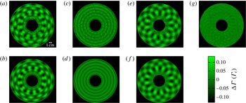
, we first subtract a background image (obtained by averaging all eight phases) and then use the linear fit shown in figure 3 to convert the light intensity values to local surfactant density values at each pixel. A sample image is shown in figure 4(a), with the brighter areas corresponding to higher surfactant density.
Sample FI composite image. (a) Image showing
 ${\rm\Delta}{\it\Gamma}$
from the
 $i=2$
stroboscopic phase of experiment 1, smoothed by a Gaussian filter of
 ${\it\sigma}=0.04~\text{cm}$
. (b) The corresponding
 ${\rm\Delta}{\it\Gamma}_{T}$
, the best fit to (2.2). (c) The meniscus wave (harmonic) component and (e) the Faraday wave (subharmonic) component of the same
 ${\rm\Delta}{\it\Gamma}$
as shown in (a). These components are isolated by adding and subtracting (and dividing by 2) the FI composite images from the
 $i=2$
and
 $i=6$
stroboscopic phases. (d) The meniscus wave (harmonic) component and (f) the Faraday wave (subharmonic) component of the same
 ${\rm\Delta}{\it\Gamma}_{T}$
as shown in (b). (g) This image is generated by subtracting (d) from (c). The resulting pattern (smoothed with a Gaussian filter of
 ${\it\sigma}=0.09~\text{cm}$
) is a higher-order mode, which is not accounted for in the ansatz (2.2). This mode has 24-fold symmetry and oscillates harmonically with peak-to-mean variation of
 $0.03~{\it\Gamma}_{c}$
.

The effects of surface curvature on the FI calibration can be separated into two parts: an increase in fluid surface area per pixel, and a change in fluorescence intensity due to the curvature itself. The former is negligible since surface tilts are so small (the slope is
 $O(10^{-3})$
), and the resulting increase in surface area is a second-order effect. Therefore, neither LED excitation nor fluorophore emission will be affected. It is possible that there are nonlinear optical effects due to the molecular conformation of the surfactants in response to the curvature, for instance by differences in mean fluorophore separation for surfaces of positive or negative curvature. Through fluorescence resonance energy transfer (Shrive et al.
Reference Shrive, Brennan, Brown and Krull1995), such conformational changes could increase/decrease the emitted light intensity depending on the sign of the curvature. We observe no evidence for such a bias in the composite data.
2.3. Moiré imaging
In order to measure the surface height field, we use an MI technique in which a reflected pattern of dark/light stripes reveals the spatial structure of the reflecting surface. For a known illumination pattern and known surface height field, a ray-tracing algorithm can produce a moiré pseudo-image, which should correspond to the observed image. To invert the moiré image, we assume a physically motivated functional form for the surface height field (see § 2.4) and search for the optimal parameters in that ansatz that best reproduce all eight observed images.
The MI system consists of an Andor Luca-R camera which images the surface height field through a hole in the mask that creates the patterned light source (see figure 1). The light source pattern is a transparent film printed with a set of concentric black rings of width 1.27 cm, chosen to be close to the wavelengths under consideration. This film, as well as a green gel filter (Lee Filters 736 Twickenham Green, with a peak transmission wavelength of
 $525\pm 50~\text{nm}$
), are sandwiched between two panes of diffusing ground glass. Two 500 W incandescent bulbs, positioned above and to the sides of the pattern (outside of the plastic tent), illuminate the fluid surface through this target pattern. Owing to the angle of the lights and the gel filters (see schematic in figure 1), most of the light intensity does not reach the fluid surface. We estimate that the resulting temperature rise inside the tent is approximately
 $1\,^{\circ }\text{C}$
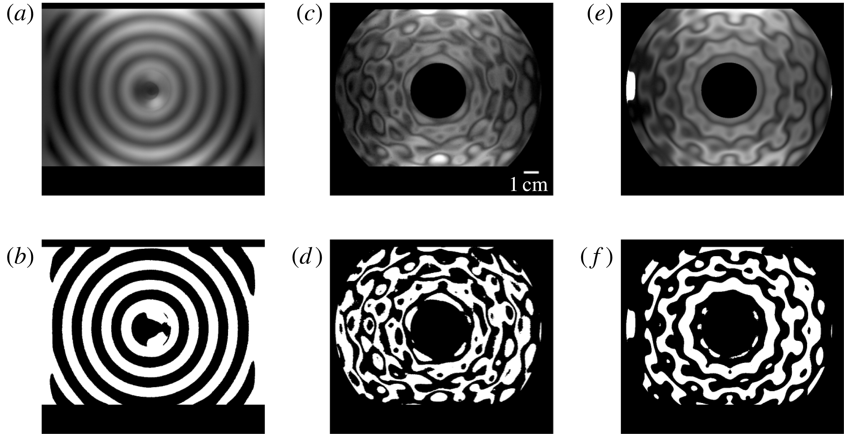
. Even though the camera is focused on the fluid surface in order to optimize the low-intensity fluorescence measurements, the short focal length (35 mm) relative to the distance to the focal plane (67.8 cm) allows the use of a ray-tracing protocol to deduce the surface height profile. Sample images of the patterned light source, MI images and best-fitting ray trace are shown in figure 5. To reduce the number of rays that trace back to either the camera or outside the patterned light source, we use the same annular field of view considered for the FI images.
Sample MI images. (a) Contrast-enhanced image and (b) binarization of the target pattern reflected off a flat fluid surface. (c) Contrast-enhanced moiré image and (d) binarization of the target pattern reflected off the fluid surface at phase
 $i=2$
for experiment 1. (e) Ray-traced pseudo-image and (f) binarization of the best-fitting
 $h(\boldsymbol{r})$
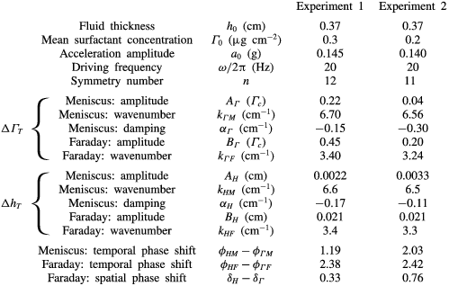
for image (c) using parameters given in table 1.

Although the axes of the camera, pattern and container are approximately aligned, we find it necessary to calculate their relative positions and orientations in order to achieve good ray-tracing results. To obtain the camera position and orientation, we image a set of metal posts of known height and spacing; to measure the centre of the target pattern, we image the reflection off of the flat fluid surface. Using these data, we calculate the spatial resolution of the camera to be
 $0.0153~\text{cm}~\text{pixel}^{-1}$
. To obtain the pixel coordinates of the system origin to subpixel resolution, we find the centre of the meniscus wave pattern in composite data which have not been corrected for the Faraday wave rotation. The pattern in the rotation-uncorrected composite data is nearly identical to that in figure 4(c).
To find the best-fitting parameters of the ansatz for
 $h(\boldsymbol{r},t)$
, we maximize the cross-correlation between the MI images and ray-traced pseudo-images. The ray-tracing protocol assumes that each ray corresponds to a pixel and all the rays start at a single point (the location of the camera). The rays are assumed to reflect off the fluid surface at the
 $z=0$
plane, a justifiable assumption since the height of the wave peaks (
 $\mathit{O}(10~{\rm\mu}\text{m})$
) is much less than the distance between neighbouring peaks (
 $\mathit{O}(1~\text{cm})$
). When waves are present, the normal to the surface changes orientation and the reflected ray responds accordingly. Each pixel of the ray-traced pseudo-images is assigned the intensity of the moiré pattern at the pixel nearest the intersection of the ray and the plane of the pattern. For the few rays that trace back outside of the patterned light source, we assign the maximum intensity recordable by the camera. We account for motion blur due to the oscillation of the wave by averaging three ray-tracing results for each of the eight MI images.
2.4. Surface height field and surfactant density field ansatz
In order to compare
 ${\rm\Delta}h$
and
 ${\rm\Delta}{\it\Gamma}$
, we use a physically motivated ansatz that allows us to measure amplitudes, wavenumbers and phases for the waves. In addition, we assume that
 ${\rm\Delta}h$
and
 ${\rm\Delta}{\it\Gamma}$
are a linear superposition of the Faraday and the meniscus waves. Our results will indicate that this assumption accounts for the most significant signals in the data. To distinguish the ansatz from the measured MI and FI data, we use the subscript
 $T$
for the ansatz quantities.
Meniscus waves take the form of a superposition of inward- and outward-travelling Hankel functions (Saylor et al.
Reference Saylor, Szeri and Foulks2000). The inward-propagating meniscus wave takes the form
 $\text{Re}[\text{e}^{\text{i}{\it\omega}t}\text{H}_{0}^{(1)}(kr)]$
, where the complex-valued wavenumber
 $k=k_{M}+\text{i}{\it\alpha}$
measures both the spatial wavenumber
 $k_{M}$
and the damping factor
 ${\it\alpha}$
. Once at the centre, the waves continue to propagate outwards according to the form
 $\text{Re}[\text{e}^{\text{i}{\it\omega}t}\text{H}_{0}^{(2)}(kr)]$
. The resulting superposition is
 $\text{Re}[\text{e}^{\text{i}{\it\omega}t}\text{J}_{0}(kr)]$
.
Sinusoidally driven Faraday waves on an uncontaminated surface of an infinitely deep inviscid fluid (Benjamin & Ursell Reference Benjamin and Ursell1954) or finite-depth low-viscosity fluid (Edwards & Fauve Reference Edwards and Fauve1994) take the form of a Bessel function
 $\text{J}_{n}(k_{F}r)\cos (n{\it\theta})\cos ({\textstyle \frac{1}{2}}{\it\omega}t)$
, where
 ${\it\omega}$
is the driving frequency and the spatial wavenumber
 $k_{F}$
is purely real. We allow for the Bessel mode to be displaced from the centre of the container, to account for the observed rotational instability, and use cylindrical coordinates measured with respect to the pattern centre rather than the axis of the experiment.
Assuming a linear superposition of the meniscus and Faraday waves, our ansatz for
 ${\rm\Delta}h$
is given by
 $$\begin{eqnarray}\displaystyle {\rm\Delta}h_{T}(r,{\it\theta},t) & = & \displaystyle h(r,{\it\theta},t)-h_{0}\nonumber\\ \displaystyle & = & \displaystyle {\rm\Delta}h_{MT}(r,t)+{\rm\Delta}h_{FT}(r^{\prime },{\it\theta}^{\prime },t)\nonumber\\ \displaystyle & = & \displaystyle A_{H}\text{Re}[\text{e}^{\text{i}({\it\omega}t+{\it\phi}_{HM})}\text{J}_{0}((k_{HM}+\text{i}{\it\alpha}_{H})r)]\nonumber\\ \displaystyle & & \displaystyle +\,B_{H}\cos ({\textstyle \frac{1}{2}}{\it\omega}t+{\it\phi}_{HF})\text{J}_{n}(k_{HF}r^{\prime })\cos (n{\it\theta}^{\prime }+{\it\delta}_{H}),\end{eqnarray}$$
where the subscripts
 $M$
and
 $F$
indicate whether the parameter is associated with the meniscus wave or the Faraday wave, respectively. The primed coordinates are relative to the centre of the Faraday wave instead of the axis of the system.
Miles (Reference Miles1967) predicts that
 ${\rm\Delta}{\it\Gamma}_{T}$
of a gravity–capillary wave is proportional to the Laplacian of the velocity potential, which is in turn proportional to
 ${\rm\Delta}h_{T}$
(Lamb Reference Lamb1945). Therefore, our
 ${\rm\Delta}{\it\Gamma}$
ansatz takes the same form as (2.1):
 $$\begin{eqnarray}\displaystyle {\rm\Delta}{\it\Gamma}_{T}(r,{\it\theta},t) & = & \displaystyle {\it\Gamma}(r,{\it\theta},t)-{\it\Gamma}_{0}\nonumber\\ \displaystyle & = & \displaystyle {\rm\Delta}{\it\Gamma}_{MT}(r,t)+{\rm\Delta}{\it\Gamma}_{FT}(r^{\prime },{\it\theta}^{\prime },t)\nonumber\\ \displaystyle & = & \displaystyle A_{{\it\Gamma}}\text{Re}[\text{e}^{\text{i}({\it\omega}t+{\it\phi}_{{\it\Gamma}M})}\text{J}_{0}((k_{{\it\Gamma}M}+\text{i}{\it\alpha}_{{\it\Gamma}})r)]\nonumber\\ \displaystyle & & \displaystyle +\,B_{{\it\Gamma}}\cos ({\textstyle \frac{1}{2}}{\it\omega}t+{\it\phi}_{{\it\Gamma}F})\text{J}_{n}(k_{{\it\Gamma}F}r^{\prime })\cos (n{\it\theta}^{\prime }+{\it\delta}_{{\it\Gamma}}).\end{eqnarray}$$
Note that
 ${\rm\Delta}{\it\Gamma}_{FT}$
can be separated into independent spatial and temporal factors. In § 3, we will test whether the temporal dynamics of
 ${\rm\Delta}{\it\Gamma}_{F}$
follow the assumed
 $\cos ({\textstyle \frac{1}{2}}{\it\omega}t)$
behaviour.
These Bessel modes for
 ${\rm\Delta}h$
and
 ${\rm\Delta}{\it\Gamma}$
are solutions to the linearized Navier–Stokes equations (Benjamin & Ursell Reference Benjamin and Ursell1954; Miles Reference Miles1967; Lucassen-Reynders & Lucassen Reference Lucassen-Reynders and Lucassen1970). In the presence of nonlinear effects such as the Benjamin–Feir instability, these solutions are not exact; however, for small-amplitude waves, the nonlinearity is small. In our experiments,
 $Ak\approx 0.01{-}0.1$
, which means that the
 $\mathit{O}((Ak)^{3})$
nonlinearity is a very small effect. Furthermore, the damping effect of the surfactant both suppresses the Benjamin–Feir instability and affects the relative phase (Segur et al.
Reference Segur, Henderson, Carter, Hammack, Li, Pheiff and Socha2005; Henderson, Segur & Carter Reference Henderson, Segur and Carter2010; Kharif & Touboul Reference Kharif and Touboul2010; Touboul & Kharif Reference Touboul and Kharif2010; Akers Reference Akers2012; Henderson & Segur Reference Henderson and Segur2013).
The nine fitting parameters in (2.1) (and the corresponding nine in (2.2)) each have a physical interpretation. To distinguish the parameters of
 ${\rm\Delta}h_{T}$
and
 ${\rm\Delta}{\it\Gamma}_{T}$
, we denote their parameters with the subscript
 $H$
and
 ${\it\Gamma}$
, respectively. The amplitudes of the meniscus and Faraday waves are given by
 $A_{H}$
and
 $B_{H}$
, respectively. The spatial wavenumbers of the pattern are:
 $k_{HM}$
and
 $k_{HF}$
(real, radial for both waves),
 ${\it\alpha}$
(imaginary, radial for meniscus wave) and
 $n$
(real, azimuthal for Faraday wave). The value of
 ${\it\alpha}$
corresponds to the energy damping rate of the meniscus wave. Only the relative phase between
 ${\rm\Delta}{\it\Gamma}$
and
 ${\rm\Delta}h$
is independent; we report temporal phase shifts for both the meniscus wave (
 ${\it\phi}_{HM}-{\it\phi}_{{\it\Gamma}M}$
) and the Faraday wave (
 ${\it\phi}_{HF}-{\it\phi}_{{\it\Gamma}F}$
). Finally, there is also a spatial phase shift for the Faraday waves (
 ${\it\delta}_{H}-{\it\delta}_{{\it\Gamma}}$
).
Owing to the high dimensionality of the parameter space, finding a best fit to this ansatz takes place in several stages, described below. The full set of fitting parameters for both
 ${\rm\Delta}h_{T}$
and
 ${\rm\Delta}{\it\Gamma}_{T}$
are provided in table 1, and discussed in detail in § 3.


First, we decompose the FI images into a harmonic component (to fit the meniscus wave terms) and a subharmonic component (Faraday wave terms) (see figure 4(c,e)). This can be done by simply adding or subtracting images that are precisely one half Faraday wave period apart (e.g. images taken at phase
 $i=1$
added to/subtracted from images taken at
 $i=5$
). We use a Levenberg–Marquardt algorithm to fit the resulting meniscus series and Faraday series to the corresponding terms in (2.2). A sample comparison of the FI composite data and the best-fitting
 ${\rm\Delta}{\it\Gamma}_{T}$
are shown in figure 4(b,d,f).
Solving the inverse problem using the MI images is more challenging, and starts from an initial
 ${\rm\Delta}h_{T}$
chosen using the fluorescence-determined wavenumbers (with the missing parameters chosen by hand). Using MATLAB fminsearch, we simultaneously maximize the cross-correlation of all eight MI images against their corresponding ray-traced pseudo-images. To minimize the effects of pattern noise on the cross-correlation, we binarize and then Gaussian-blur both the MI image and the ray-traced pseudo-image before performing the cross-correlation. The searching algorithm proceeds by varying the parameters in (2.1) until a best fit is found. A sample image is shown in figure 5, illustrating that we are able to fit even small features of the surface waves.
3. Results
We present direct measurements of the spatiotemporal dynamics of a surfactant monolayer on gravity–capillary waves. In figures 4 and 5, we showed that our measurements of deviations of the surface height field
 ${\rm\Delta}h$
and surfactant density field
 ${\rm\Delta}{\it\Gamma}$
are well approximated by a linear superposition of a Faraday wave and a meniscus wave, each represented by a Bessel function. Equations (2.1) and (2.2), together with the parameters provided by fits to the data (see table 1), allow us to examine the spatiotemporal dynamics in detail.
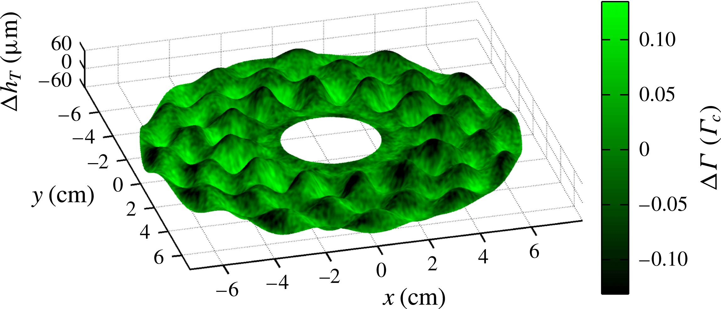
In figures 6–8, we present three-dimensional visualizations of the complete
 ${\rm\Delta}h$
and
 ${\rm\Delta}{\it\Gamma}$
fields (a snapshot at a single phase), as well as the same data split into its meniscus and Faraday wave components. In each case, the best-fitting
 ${\rm\Delta}h_{T}$
is shown as a surface mesh, with the colouring representing the measured
 ${\rm\Delta}{\it\Gamma}$
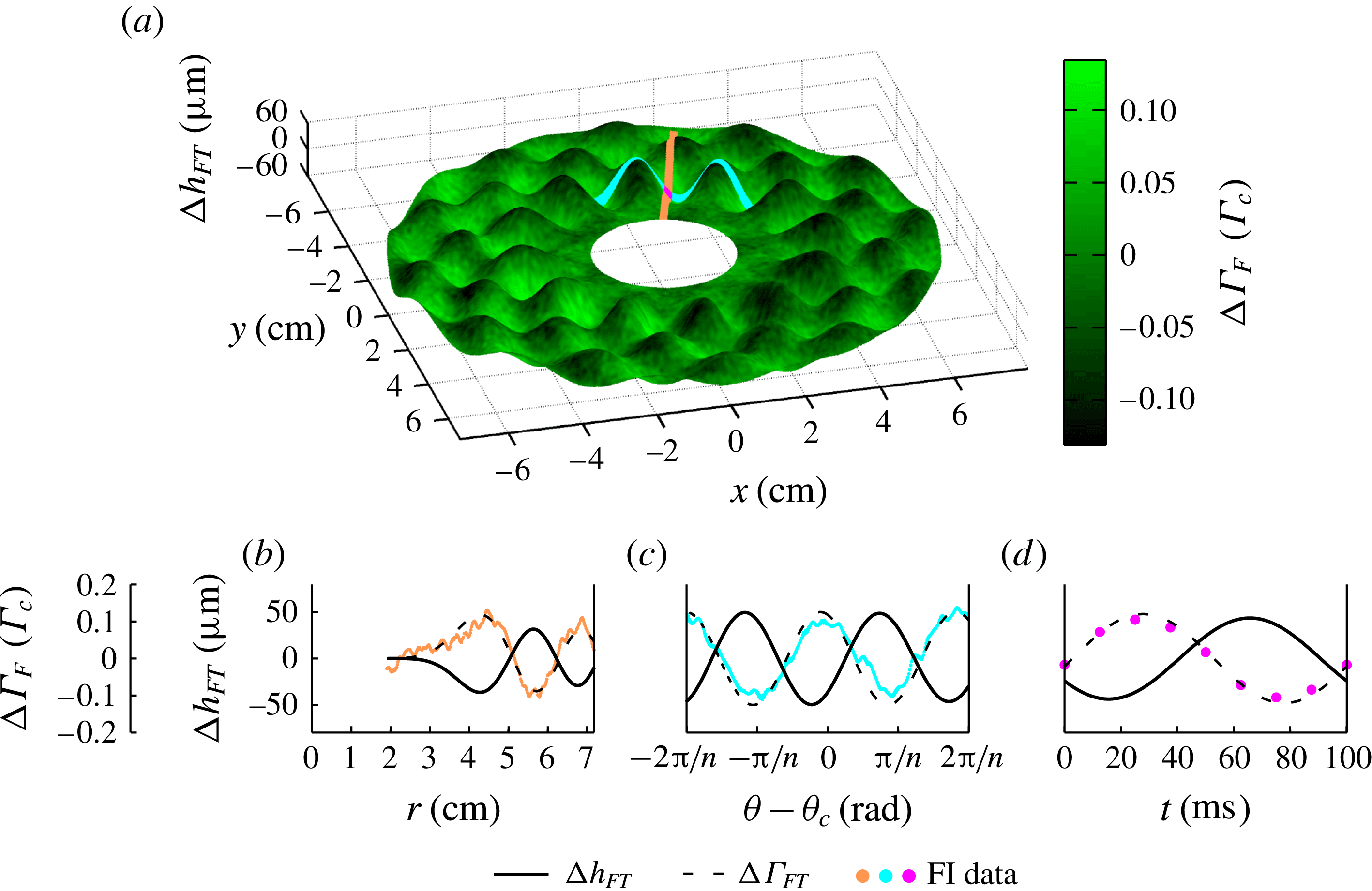
: bright green regions are rich in surfactant, while dark green are depleted. Movie versions of these figures, showing all eight phases, can be found in the online supplementary material available at http://dx.doi.org/10.1017/jfm.2015.352. Below, we compare observations about both the travelling meniscus waves and the standing Faraday waves, along with the weaker higher-order mode observed in the FI composite data.
Visualization of
 ${\rm\Delta}h_{T}$
and
 ${\rm\Delta}{\it\Gamma}$
for experiment 1, within the annular field of view. The best fit using the
 $h$
ansatz (2.1) (mesh surface) and the FI composite data (colouration) for the
 $i=2$
stroboscopic phase. The peak-to-mean variations in
 ${\rm\Delta}h_{T}$
and
 ${\rm\Delta}{\it\Gamma}_{T}$
are
 $\pm 60~{\rm\mu}\text{m}$
and
 $\pm 0.15~{\it\Gamma}_{c}$
, respectively. The
 ${\rm\Delta}{\it\Gamma}$
field is smoothed by a Gaussian filter of
 ${\it\sigma}=0.04~\text{cm}$
to reduce noise. In figures 7 and 8, these same data are decomposed into meniscus and Faraday wave components. A video version of this plot is available in the online supplementary movie.

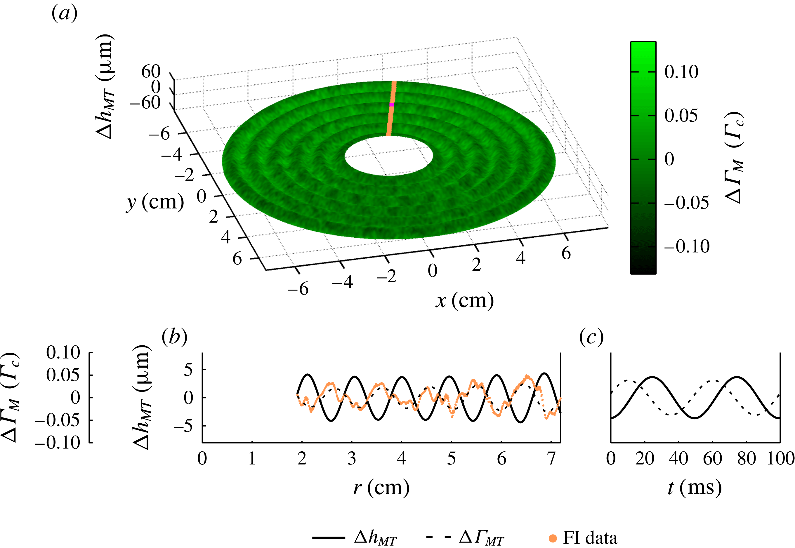
Meniscus wave component of
 ${\rm\Delta}h_{T}$
and
 ${\rm\Delta}{\it\Gamma}$
for experiment 1. (a) The best-fitting
 ${\rm\Delta}h_{MT}$
ansatz from (2.1) (mesh surface) and the harmonic component of
 ${\rm\Delta}{\it\Gamma}$
(colouration) for the
 $i=2$
stroboscopic phase. (b) Radial slice of both fields along
 ${\it\theta}=2.83~\text{rad}$
, the orange strip shown in (a), at phase
 $i=2$
. The solid line is the best-fitting height field
 ${\rm\Delta}h_{MT}(r)$
, and the surfactant density field is shown both as the data
 ${\rm\Delta}{\it\Gamma}_{M}$
(orange points) and as the ansatz
 ${\rm\Delta}{\it\Gamma}_{MT}$
(dashed line). The lines are the Bessel modes given in (2.1) and (2.2). (c) The temporal dynamics of
 ${\rm\Delta}h_{MT}$
(solid line) and
 ${\rm\Delta}{\it\Gamma}_{MT}$
(dashed line) at the location
 $r=4.79~\text{cm}$
and
 ${\it\theta}=2.83~\text{rad}$
, marked by the magenta dot in (a). The lines are the sinusoids given in (2.1) and (2.2). In all cases, the
 ${\rm\Delta}{\it\Gamma}$
fields are smoothed by a Gaussian filter of
 ${\it\sigma}=0.04~\text{cm}$
to reduce noise. A video version of this plot is available in the online supplementary movie.

Faraday wave component of
 ${\rm\Delta}h_{T}$
and
 ${\rm\Delta}{\it\Gamma}$
for experiment 1. (a) The best-fitting
 $h_{FT}$
ansatz from (2.1) (mesh surface) and the subharmonic component of
 ${\rm\Delta}{\it\Gamma}$
(colouration) for the
 $i=2$
stroboscopic phase. (b) Radial slice of both fields along
 ${\it\theta}_{c}=2.83$
rad, the orange strip shown in (a), at phase
 $i=2$
. The solid line is the best-fitting height field
 ${\rm\Delta}h_{FT}(r,{\it\theta}_{c})$
, and the surfactant density field is shown both as the data
 ${\rm\Delta}{\it\Gamma}_{F}$
(orange points) and as the ansatz
 ${\rm\Delta}{\it\Gamma}_{FT}$
(dashed line). The lines are the Bessel modes given in (2.1) and (2.2). (c) Azimuthal slice of both fields along
 $r_{c}=4.26~\text{cm}$
, the cyan strip shown in (a), at phase
 $i=2$
. Here, the surfactant density field data
 ${\rm\Delta}{\it\Gamma}_{F}$
are represented with cyan points. The lines are the sinusoids given in (2.1) and (2.2) and plotted within a restricted range of the azimuthal dimension
 $[-2{\rm\pi}/n,2{\rm\pi}/n]$
centred about
 ${\it\theta}_{c}$
. (d) The temporal dynamics of
 ${\rm\Delta}h_{FT}$
(solid line) and
 ${\rm\Delta}{\it\Gamma}_{FT}$
(dashed line) at the location
 $r_{c}~\text{cm}$
and
 ${\it\theta}_{c}$
rad, marked by the magenta dot in (a). The lines are the sinusoids given in (2.1) and (2.2). The magenta circles in (d) plot the behaviour of
 ${\mathcal{T}}(t)$
given in (3.1), with error bars much smaller than the symbol size. The
 ${\rm\Delta}{\it\Gamma}$
fields in (a–c) are smoothed by a Gaussian filter of
 ${\it\sigma}=0.04~\text{cm}$
to reduce noise. A video version of this plot is available in the online supplementary movie.

For the meniscus waves, we observe that the surfactant accumulates on the leading edge of the travelling wave, as shown in figure 7(c), where the dashed line (
 ${\rm\Delta}{\it\Gamma}_{MT}$
) leads the solid line (
 ${\rm\Delta}h_{MT}$
). The fields
 ${\rm\Delta}h$
and
 ${\rm\Delta}{\it\Gamma}$
both exhibit a Bessel
 $\text{J}_{0}$
mode, and the real parts of the associated wavenumbers
 $k_{HM}$
and
 $k_{{\it\Gamma}M}$
agree, as expected. We also observe the expected sinusoidal temporal dynamics predicted by Saylor et al. (Reference Saylor, Szeri and Foulks2000) and Picard & Davoust (Reference Picard and Davoust2006). The maximum peak-to-mean variations in
 ${\rm\Delta}h_{MT}$
, measured within our annular field of view, are 5 and
 $8~{\rm\mu}\text{m}$
for experiments 1 and 2, respectively. The corresponding values for
 ${\rm\Delta}{\it\Gamma}_{MT}$
are 0.05 and
 $0.02~{\it\Gamma}_{c}$
. These variations in
 ${\rm\Delta}{\it\Gamma}_{MT}$
correspond to variations in the surface tension of 0.5 and
 $1.5~\text{mN}~\text{m}^{-1}$
, respectively (Tsukanova et al.
Reference Tsukanova, Grainger and Salesse2002). The location of the surfactant relative to the fluid wave corresponds to a temporal phase shift between
 ${\rm\Delta}h_{MT}$
and
 ${\rm\Delta}{\it\Gamma}_{MT}$
, shown in figure 7(c).
For the Faraday waves, we observe that the surfactant accumulates in the troughs of the standing wave, as shown in figure 8(d), where the dashed line (
 ${\rm\Delta}{\it\Gamma}_{FT}$
) leads the solid line (
 ${\rm\Delta}h_{FT}$
). The fields
 ${\rm\Delta}h$
and
 ${\rm\Delta}{\it\Gamma}$
both exhibit a Bessel
 $\text{J}_{n}$
mode, and the wavenumbers
 $k_{HF}$
and
 $k_{{\it\Gamma}F}$
agree, as expected (Miles Reference Miles1967). We note that the wavenumber of the Faraday wave is roughly double that for the meniscus wave, and the values of the wavenumbers can be captured by the finite-depth Kelvin dispersion relation,
 ${\it\omega}^{2}=(gk+{\it\sigma}k^{3}/{\it\rho})\tanh (h_{0}k)$
, when the accepted values for the acceleration due to gravity
 $g$
and density of water
 ${\it\rho}$
are used and the same surface tension is left as a fitting parameter. The best-fitting surface tensions for experiments 1 and 2 are 33.3 and
 $35.6~\text{mN}~\text{m}^{-1}$
, respectively. The fields
 ${\rm\Delta}h$
and
 ${\rm\Delta}{\it\Gamma}$
both exhibit a sinusoidal azimuthal behaviour with the same symmetry
 $n$
as well as a sinusoidal temporal dynamics at half the driving frequency. The maximum peak-to-mean variations in
 ${\rm\Delta}h_{FT}$
, measured within our annular field of view, are 62 and
 $64~{\rm\mu}\text{m}$
for experiments 1 and 2, respectively. The corresponding values for
 ${\rm\Delta}{\it\Gamma}_{FT}$
are
 $0.13$
and
 $0.06~{\it\Gamma}_{c}$
. These variations in
 ${\rm\Delta}{\it\Gamma}_{FT}$
correspond to variations in the surface tension of 1.5 and
 $3.5~\text{mN}~\text{m}^{-1}$
, respectively (Tsukanova et al.
Reference Tsukanova, Grainger and Salesse2002). Similar magnitudes in the variations of the surface tension have been observed for 1 Hz gravity waves contaminated with various molecular monolayers (Lange & Hühnerfuss Reference Lange and Hühnerfuss1984). The location of the surfactant relative to the fluid wave corresponds to a temporal phase shift between
 ${\rm\Delta}h_{FT}$
and
 ${\rm\Delta}{\it\Gamma}_{FT}$
, shown in figure 8(d). We also observe a small but non-negligible spatial phase shift (
 ${\it\delta}_{H}-{\it\delta}_{{\it\Gamma}}$
) between
 ${\rm\Delta}{\it\Gamma}_{FT}$
and
 ${\rm\Delta}h_{FT}$
equal to 0.33 and 0.76 rad for experiments 1 and 2, respectively. This spatial phase shift is in the same direction as the rotation of the Faraday wave pattern in both experiments.
We have also considered a stricter test of the temporal dynamics for
 ${\rm\Delta}{\it\Gamma}$
of the Faraday waves to determine whether they evolve non-sinusoidally, as indicated by the numerical solutions of Ubal et al. (Reference Ubal, Giavedoni and Saita2005). As given in (2.2), the ansatz for
 ${\rm\Delta}{\it\Gamma}_{F}$
can be factored into
 ${\mathcal{S}}_{T}(r^{\prime },{\it\theta}^{\prime }){\mathcal{T}}_{T}(t)$
, where the spatial factor is given by
 ${\mathcal{S}}_{T}(r^{\prime },{\it\theta}^{\prime })\equiv B_{{\it\Gamma}}\text{J}_{n}(k_{{\it\Gamma}F}r^{\prime })\cos (n{\it\theta}^{\prime }+{\it\delta}_{{\it\Gamma}})$
and the temporal factor by
 ${\mathcal{T}}_{T}(t)\equiv \cos ({\textstyle \frac{1}{2}}{\it\omega}t+{\it\phi}_{{\it\Gamma}F})$
. The subscript
 $T$
denotes that these quantities are fits to the ansatz, rather than the data. Since the spatial factor is well characterized by the ansatz (
 ${\mathcal{S}}={\mathcal{S}}_{T}$
), as shown in figures 4(e,f) and 8(b,c), we can isolate the temporal dynamics of
 ${\rm\Delta}{\it\Gamma}_{F}$
for the data by considering the quantity
 $$\begin{eqnarray}{\mathcal{T}}(t)=\left\langle \frac{{\rm\Delta}{\it\Gamma}_{F}(r^{\prime },{\it\theta}^{\prime },t)}{{\mathcal{S}}_{T}(r^{\prime },{\it\theta}^{\prime })}\right\rangle ,\end{eqnarray}$$
where the angle brackets denote an average over all space (approximately
 $5\times 10^{5}$
pixels in total). In performing the average, we exclude pixels where
 $|{\mathcal{S}}_{T}(r^{\prime },{\it\theta}^{\prime })|<0.006~{\it\Gamma}_{c}$
to avoid the calculation being badly conditioned. As shown in figure 8(d), the average temporal dynamics
 ${\mathcal{T}}(t)$
(and therefore the temporal dynamics of
 ${\rm\Delta}{\it\Gamma}_{F}$
) is well described by a sinusoidal function.
Our ansatz assumes a linear superposition of the meniscus and Faraday waves. While this ansatz captures most of the total pattern, there is a residual mode in the FI data (see figure 4(g)) that generates peak-to-mean variations in
 ${\rm\Delta}{\it\Gamma}$
of
 $0.03$
and
 $0.01~{\it\Gamma}_{c}$
for experiments 1 and 2, respectively. This higher-order mode probably arises through a nonlinear interaction between the meniscus and Faraday waves such as those that give rise to the Benjamin–Feir instability (Segur et al.
Reference Segur, Henderson, Carter, Hammack, Li, Pheiff and Socha2005; Henderson et al.
Reference Henderson, Segur and Carter2010; Kharif & Touboul Reference Kharif and Touboul2010; Touboul & Kharif Reference Touboul and Kharif2010; Akers Reference Akers2012; Henderson & Segur Reference Henderson and Segur2013). Although this mode has a Bessel mode shape like the Faraday waves (
 $F(r,{\it\theta})\sim \text{J}_{m}(kr)\cos (n{\it\theta}+{\it\phi})$
) with
 $m=2n$
(twice the symmetry number of the fundamental mode), the distance between neighbouring extrema is comparable to that of the meniscus waves. Additionally, the higher mode is harmonic in time, unlike the subharmonic Faraday wave.
We observe that the degree of surfactant mobility depends on the type of wave. By comparing the
 ${\it\Gamma}$
amplitudes of the associated Faraday versus meniscus Bessel modes
 $(B_{{\it\Gamma}}/A_{{\it\Gamma}})$
, we find a ratio of 2 for experiment 1, and 5 for experiment 2. This indicates that Faraday waves have a larger effect than meniscus waves. However, if the
 ${\it\Gamma}$
amplitudes are rescaled by the associated
 $h$
amplitudes, then meniscus waves have proportionally larger effect: the ratio
 $(B_{{\it\Gamma}}/B_{H})/(A_{{\it\Gamma}}/A_{H})$
is 0.21 for experiment 1, and 0.78 for experiment 2. The cause of these differences is unclear and could be due to the difference between travelling versus standing waves, to the difference in oscillation frequency, or to some subtlety of nonlinearity. In contrast, the observed differences between the two experiments is clear and indicates that material mobility depends on
 ${\it\Gamma}_{0}$
.
There are other subtle differences between the two experiments, suggesting an array of rich dynamics that depend on the mean surfactant concentration. First, the temporal phase shifts
 ${\rm\Delta}{\it\phi}={\it\phi}_{H}-{\it\phi}_{{\it\Gamma}}$
are consistent for the Faraday waves across both experiments, but differ for the meniscus waves. Furthermore, only
 ${\rm\Delta}{\it\phi}_{M}$
for experiment 1 is less than
 ${\rm\pi}/2$
rad, the expected maximum temporal phase shift for linear gravity–capillary waves (Lucassen-Reynders & Lucassen Reference Lucassen-Reynders and Lucassen1970). Second, the two damping factors (
 ${\it\alpha}_{H}$
and
 ${\it\alpha}_{{\it\Gamma}}$
, both associated with the travelling meniscus wave) agree for experiment 1 but not for experiment 2. From the theoretical predictions of Picard & Davoust (Reference Picard and Davoust2006), we would expect agreement.
4. Conclusions
We have successfully developed a novel technique for measuring the surface height
 $h$
and surfactant density
 ${\it\Gamma}$
fields for waves propagating on a surfactant-covered fluid. We observe that the surfactant accumulates on the leading edge of travelling meniscus waves and the troughs of standing Faraday waves. The deviations of both the surface height field
 ${\rm\Delta}h$
and surfactant density field
 ${\rm\Delta}{\it\Gamma}$
take characteristic Bessel forms for both the meniscus and Faraday waves. For the meniscus waves, both fields follow a
 $\text{J}_{0}$
Bessel mode, but are temporally phase shifted from each other. For the Faraday waves, both fields follow the same
 $\text{J}_{n}$
Bessel mode, but are both temporally and spatially phase shifted from each other.
For meniscus waves, Saylor et al. (Reference Saylor, Szeri and Foulks2000) and Picard & Davoust (Reference Picard and Davoust2006) have analytically derived
 ${\rm\Delta}h$
and
 ${\rm\Delta}{\it\Gamma}$
. These two fields are expected to share the same functional form up to a complex-valued coefficient (
 $F(r,t)=F_{0}\text{J}_{0}(kr)\text{e}^{\text{i}{\it\omega}t}$
where
 $k=k_{M}+\text{i}{\it\alpha}$
) and therefore are expected to have the same wavenumbers and damping factors. However, this work does not predict the relationship between the values of
 $F_{0}$
for the two fields, which would be necessary to understand the temporal phase shifts. Lucassen-Reynders & Lucassen (Reference Lucassen-Reynders and Lucassen1970) studied two-dimensional travelling gravity–capillary waves in a Cartesian geometry, and derived a prediction for the phase shift between the surface area expansion and
 ${\rm\Delta}h$
. For
 ${\it\Gamma}$
inversely proportional to the area of the fluid surface, the temporal phase shift between
 ${\rm\Delta}h$
and
 ${\rm\Delta}{\it\Gamma}$
is predicted to fall between 0 and
 ${\rm\pi}/2$
rad depending on the surface compression modulus. This corresponds to the surfactant accumulating somewhere between the crests of the waves and the leading edge.
In experiment 2, we observe
 ${\it\phi}_{HM}-{\it\phi}_{{\it\Gamma}M}>{\rm\pi}/2$
rad and
 ${\it\alpha}_{H}\neq {\it\alpha}_{{\it\Gamma}}$
, both of which suggest that we may be exciting longitudinal waves in the system. Longitudinal waves, like gravity–capillary waves, are a solution to the linearized Navier–Stokes equations for incompressible fluids. By including the effect of the surfactant through the normal and tangential stress boundary condition, Lucassen (Reference Lucassen1968a
) derived a dispersion relation, one branch of which corresponds to gravity–capillary waves, which have roughly equal parts transverse and tangential to motion of the interface, and the other branch of which corresponds to longitudinal (i.e. Marangoni) waves, which have significantly more tangential motion than transverse (Lucassen-Reynders & Lucassen Reference Lucassen-Reynders and Lucassen1970). If our system produced transverse and longitudinal meniscus waves, they would both be
 $\text{J}_{0}$
Bessel modes. Our technique for measuring
 ${\rm\Delta}{\it\Gamma}$
would measure a superposition of both waves and the value of
 ${\it\alpha}_{{\it\Gamma}}$
used in the fitting ansatz would be increased. Because longitudinal waves do not significantly perturb
 ${\rm\Delta}h$
, the damping factor for
 ${\rm\Delta}h$
would be unchanged. Consequently, the presence of a longitudinal wave in the system would look like
 ${\it\alpha}_{{\it\Gamma}}>{\it\alpha}_{H}$
, as in our observations. The possibility of a gravity–capillary wave resonantly exciting a longitudinal wave was first suggested by Lucassen (Reference Lucassen1968a
) because the maximum in energy dissipation coincides with the equality of the magnitude of the gravity–capillary and longitudinal wavenumbers. Recently, Ermakov (Reference Ermakov2003) proposed a mechanism for this resonant excitation that would explain the coincidence of damping with the wavenumber equality. Future experiments that measure
 ${\rm\Delta}{\it\Gamma}$
would be able to test this mechanism.
The discrepancies in the measured values of
 ${\it\alpha}$
highlight the importance of quantifying the surface dilatational viscosity, dilatational elasticity and surface tension (collectively, the interfacial rheology). Historically, techniques for measuring the interfacial rheology have relied on extracting the wavenumber and damping factor from the surface height field
 $h$
of a travelling gravity–capillary wave (Miyano et al.
Reference Miyano, Abraham, Ting and Wasan1983; Jiang et al.
Reference Jiang, Chiew and Valentini1993; Saylor et al.
Reference Saylor, Szeri and Foulks2000; Behroozi et al.
Reference Behroozi, Cordray, Griffin and Behroozi2007). The experiments described here provide a way to make a more direct measurement, using the
 ${\it\Gamma}$
field in addition to the
 $h$
field.
For Faraday waves, there is theoretical literature relating the interaction between a surfactant monolayer and a Faraday wave in a fluid of arbitrary depth (Kumar & Matar Reference Kumar and Matar2002, Reference Kumar and Matar2004; Ubal et al.
Reference Ubal, Giavedoni and Saita2005; Martín & Vega Reference Martín and Vega2006). Kumar & Matar (Reference Kumar and Matar2002, Reference Kumar and Matar2004) assumed that, in an infinitely broad fluid, both
 ${\rm\Delta}h$
and
 ${\rm\Delta}{\it\Gamma}$
oscillate sinusoidally and with zero temporal phase shift. They also predicted a spatial phase shift between the two fields. In the experimental data, we observe sinusoidal oscillations, but with a temporal phase shift of approximately 2.4 rad. However, we confirm the spatial phase shift (
 ${\it\delta}_{H}-{\it\delta}_{{\it\Gamma}}$
in table 1). Martín & Vega (Reference Martín and Vega2006) attribute rotational drift of Faraday waves to the generation of a streaming flow, under the assumption that the two fields have no spatial or temporal phase shift. However, it is also plausible that our observed rotation of the Faraday waves is caused by the spatial phase shift. Ubal et al. (Reference Ubal, Giavedoni and Saita2005) studied the motion of
 ${\rm\Delta}h$
and
 ${\rm\Delta}{\it\Gamma}$
through numerical simulations of the two-dimensional Navier–Stokes equations with physically realistic interfaces and spatially symmetric boundary conditions in a finite-depth fluid. In agreement with our experiments, they predicted that
 ${\rm\Delta}h$
and
 ${\rm\Delta}{\it\Gamma}$
have similar spatial patterns, and that maxima in
 ${\rm\Delta}{\it\Gamma}$
would precede maxima in
 ${\rm\Delta}h$
, an effect characterized by a temporal phase shift. The prediction of peak-to-mean variations in
 ${\rm\Delta}{\it\Gamma}\approx 0.03$
–
 $0.13~{\it\Gamma}_{c}$
is consistent with our observations, although for different parameters from those used in the experiment. However, their conclusion that the two fields have different non-sinusoidal time dependence does not agree with our data. Additionally, the use of spatially symmetric boundary conditions in the numerical simulations excludes the possibility of predicting the drift of the Faraday wave that we observe. Matar, Kumar & Craster (Reference Matar, Kumar and Craster2004) considered surfactant-covered Faraday waves on thin fluid films using lubrication theory. In steady state, they find that
 ${\rm\Delta}{\it\Gamma}$
is out of phase with
 ${\rm\Delta}h$
, and accumulates in the troughs of the Faraday waves. While our fluid thickness is too large for this result to apply, our observations are consistent with their findings.
For other nonlinear wave effects, such as the Benjamin–Feir instability, the phase between
 ${\rm\Delta}h$
and
 ${\rm\Delta}{\it\Gamma}$
is expected to affect the dynamic properties of the propagating waves (Akers Reference Akers2012). The experimental techniques we present here could prove valuable for future studies into these nonlinear effects.
Finally, although we have studied the wave-driven accumulation of a molecular layer of surface contamination, similar effects are known to be present for other types of surface contamination. For example, Sanlı et al. (Reference Sanlı, Lohse and van der Meer2014) used Faraday waves to redistribute a monolayer of millimetre-scale polystyrene spheres deposited on the surface. Depending on the concentration of the particulate layer, the macroscopic contaminant would accumulate in either the antinodes (peak/trough) or the nodes of the waves. This behaviour is quite different from what we observe at the molecular scale, suggesting the presence of a crossover in particle size or surface activity. Because oceanic contamination ranges in size from the molecular scale to flotsam and jetsam, more work is needed to develop a complete picture of the dynamics of contamination on surface waves.
Acknowledgements
This work was funded by the NSF, under grant number DMS-0968258. We are grateful to the West Virginia High Technology Consortium Foundation for the donation of the electromagnetic shaker and isolation table, and to R. Levy for the use of an Andor camera in the development of this work (funded by Research Corporation RCSA 19788).
Supplementary movies
Supplementary movies are available at http://dx.doi.org/10.1017/jfm.2015.352.