2.1 The problem

Suppose your company had a number of losses X ₁,…X_n over a period of k years. For each loss X_j we have the loss date LD_j and the reporting date RD_j, normally (but not always) expressed with the precision of one day. By aggregating the accident year we have n ₁,…n_k reported losses for years 1 to k. The objective is to calculate the projected number of losses N ₁,…N_k for each year:

The traditional approach to this problem is to aggregate losses in a frequency development triangle analogous to that in Fig. 1, which gives the number of losses for each accident year (rows) and for each development year (columns), then project to ultimate using a triangle projection technique, such as the chain ladder.

The main issue with this approach is that aggregating claim counts in a triangle throws away most of the information we have: e.g. if we have 1,000 losses over 10 years, we will compress the information on the reporting delay (which is made of 1,000 different numbers) into a small triangle (which is made of 55 different numbers). Bizarrely, increasing the number of losses from, say, 1,000 to 10,000 does not increase at all the information that we can use to project to the final number of claims! This information compression is helpful for visualisation purposes and made sense in an age when calculations were performed by hand, and is surprisingly resilient in terms of finding an accurate projected number of claims for each year, but it ties our hands when trying to calculate the distribution of possible outcomes, making the uncertainty difficult to assess.

In Section 2.2 we propose an alternative approach. This approach is in the same spirit as the works by Kaminsky (Reference Kaminsky1987), Weissner (Reference Weissner1978) and Guiahi (Reference Guiahi1986).

2.2 A method for frequency projection

The method we propose is based on using the distribution F(t) which gives the cumulative probability that a loss occurred at time 0 will be reported by time t.

2.2.1 The continuous case with known delay distribution F

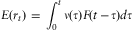
Assume first that the delay distribution F(t) is known. Assume t is the current date, and that we want to estimate the total number of claims that will ultimately be reported for the period [0,t]. Let v(t) the frequency density of claims at time t – it can also be interpreted as a risk profile – where v(t) is higher, the probability of having a claim is also higher. This may be due to seasonality (e.g. v(t) may be higher in winter) or to non-seasonal systemic effects. The total (unknown) number of claims expected to occur in [0,t] will be

$$E({{\mu }_t})\, = \,\mathop \int \sidelimits_0^t \nu \left( \tau \right)d\tau $$

The expected number of claims to be reported by time t is

$$E({{r}_t})\, = \,\mathop \int \sidelimits_0^t \nu \left( \tau \right)F(t\,{\rm{ - }}\,\tau )d\tau $$

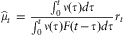
Normally r_t, the number of reported claims, will be known, whereas μ_t is to be estimated: the estimated value of μ_t, $$${{\widehat{\mu }}_t}$$$ , is given by

$${{\widehat{\mu }}_t}\, = \,\frac{{\int _0^t \nu \left( \tau \right)d\tau }}{{\int _0^t \nu \left( \tau \right)F\left( {t\,{\rm{ - }}\,\tau } \right)d\tau }}{{r}_t}$$

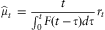
If the probability of having a claim can be assumed to be uniform, this simplifies to

$${{\widehat{\mu }}_t}\, = \,\frac{t}{{\int _0^t F\left( {t\,{\rm{ - }}\,\tau } \right)d\tau }}{{r}_t}$$

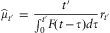
If we wish to project to ultimate the frequency for a period (0,t′) which is completely in the past (t′ < t) then it is sufficient to replace the upper limit of the integral with t′ (note that the point t inside the integral from which the CDF is calculated remains unaltered):

$${{\widehat{\mu }}_{t&#x0027;}}\, = \,\frac{{t&#x0027;}}{{\int _0^{{{t}}&#x0027;} } F\left( {t\,{\rm{ - }}\,\tau } \right)d\tau }}{{r}_{t&#x0027;}}$$

Formulae (4) and (5) have a simple geometric interpretation, which is illustrated in Fig. 6.

Figure 6

The denominator of the fraction in Equation (4) can be pictured as the gray area below the CDF and to the right of the y-axis (“Expected reported”) and the numerator as the rectangle with sides t and 1 (“Expected IBNR”+“Expected reported”). The factor to ultimate for the whole period [0,t] is therefore the ratio of the two areas. Analogously, the denominator of the fraction in Equation (6) can be pictured as the area below the CDF, between the y-axis and the axis τ = t′, and the numerator as the rectangle of sides t′ and 1. The factor to ultimate for the period [0,t′] is again the ratio of the two areas.

2.2.2 The discrete case

In practice, of course, the number of reported claims in a period [0,t] will only be known for discrete values of t, typically expressed in days: The estimated delay distribution $$$\widehat{F}(t)$$$ (more on it later) will also be a distribution known at discrete values. It is perhaps helpful, therefore, to give a discrete version of the formulae above.

In particular, if the time t is expressed in days, Equation (4) becomes

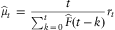$${{\widehat{\mu }}_t}\, = \,\frac{t}{{\sum _{k\, = \,0}^t \widehat{F}\left( {t\,{\rm{ - }}\,k} \right)}}{{r}_t}$$

Now if we define

$${\rm{\# }}\ {\rm{of}}\ {\rm{earned}}\ {\rm{days}}\ {\rm{in}}\,{\rm{the}}\ {\rm{period}}\ [{\rm{0}},t]\, = \,\mathop \sum \limits_{k\, = \,0}^t \widehat{F}\left( {T\,{\rm{ - }}\,k} \right)$$

We can rewrite the equation above in a much more intuitive way:

$${{\widehat{\mu }}_t}\, = \,\frac{{{\rm{\# }}\ {\rm{of}}\ {\rm{days}}\ {\rm{in}}\ {\rm{the}}\ {\rm{period}}\ {\rm{}}[0,t]}}{{{\rm{\# }}\ {\rm{of}}\ {\rm{earned}}\ {\rm{days}}\ {\rm{in}}\ {\rm{the}}\ {\rm{period}}\ [0,t]}}{{r}_t}$$

Analogously, Equation (5) becomes, in discrete time:

$${{\widehat{\mu }}_{t&#x0027;}}\, = \,\frac{{{\rm{\# }}\ {\rm{of}}\ {\rm{days}}\ {\rm{in}}\ {\rm{the}}\ {\rm{period}}\ [{\rm{0}},t&#x0027;]}}{{{\rm{\# }}\ {\rm{of}}\ {\rm{days}}\ {\rm{in}}\ {\rm{the}}\ {\rm{period}}\ \left[ {0,{{t}^&#x0027;} } \right]\ {\rm{earned}}\ {\rm{by}}\ {\rm{time}}\ {{t}}}}\,{{r}_{t&#x0027;}}$$

Fig. 7 shows an example of calculation based on formulae (8) and (9) above, in which the number of earned days is calculated either for the whole period lumped together and for different accident years separately.

Figure 7

An example of calculation for the factors to ultimate, both when all years are lumped together (top) and when the calculations are carried out separately for each individual accident year (bottom). The exposure has been assumed constant in this specific case, although this is not a necessary assumption, as the case study in Section 7 shows.

The method that lumps all years together leads to more accurate results, since the projection of isolated years is affected by large errors for the more recent years. However, in many circumstances it will be useful to identify the IBNR in the claim count for each individual year. This will also allow us to estimate the year-on-year volatility.

The problem with calculating the IBNR separately for each year is of course that the more recent years may have some numerical instability. In the most extreme case, there might be no claims at all in the last year(s), and the projection would always yield zero.

This problem is common to triangulation methods such as the chain ladder. To get around this problem one can use a credibility approach, much in the same way as it is done with Bornhuetter-Ferguson (which uses a prior estimate of the loss ratio) or by Cape-Cod (which uses an average of the previous years). Section 7.1.3 shows in detail the workings of a possible credibility approach for triangle-free reserving in a practical case.

2.2.3 Calculating the uncertainty

The standard error on the projected number of claims can be easily calculated if we can make a reasonable assumption of what the underlying claim count process is – e.g. Poisson, negative binomial, etc.

If underlying claim count process is Poisson with rate μ_t, it can be easily proved that the number of IBNR claims also follows a Poisson distribution with rate μ_t − E(r_t). Since the variance of a Poisson process is equal to its mean, the variance of the process is also μ_t − E(r_t), which can be estimated from the data as $$${{\widehat{\mu }}_t}{\rm{ - }}\,{{r}_t}$$$ . The square root of this can be used as an estimate of the standard error by which we know the ultimate claim count for the period [0,t]:

$${\rm{s}}{\rm{.e}}{\rm{.(IBNR)}}\, = \,\sqrt {{{{\widehat{\mu }}}_t}{\rm{ - }}\,{{r}_t}}$$

(Note that we are not speaking here of the standard error on the estimated Poisson rate, which would be much smaller, but of the standard error of the projected claim count. This is why we do not need to divide by the number of observations.)

In case of an overdispersed Poisson process, e.g. a negative binomial process, this method can be easily modified by setting the standard error equal to

$${\rm{s}}{\rm{.e}}{\rm{.(IBNR)}}\, = \,\sqrt {\left( {{\rm{1}}\, + \,r} \right)\left( {{{{\widehat{\mu }}}_t}\,{\rm{ - }}\,{{r}_t}} \right)} $$

where 1 + r is the variance-to-mean ratio.

2.2.4 A special case: exponential delays

It is often the case that the delay distribution can be well approximated by something simple,

e.g. an exponential distribution with average delay τ:

$$F\left( t \right)\, = \,{\rm{1 - exp}}({\rm{ - }}t/\tau )$$

In this case Equation (4) simplifies to:

$${{\widehat{\mu }}_T}(T)\, = \,\frac{T}{{T{\rm{ - }}\,\tau \left( {{\rm{1 - }}\exp \left( {{\rm{ - }}\frac{T}{\tau }} \right)} \right)}}{{r}_T}$$

and Equation (5) simplifies to:

$${{\widehat{\mu }}_T}({{T&#x0027;}} )\, = \,\frac{{T&#x0027;}}{{T&#x0027;\,{\rm{ - }}\,\tau \exp \left( {{\rm{ - }}\frac{T}{\tau }} \right)\left( {\exp \left( {\frac{{T&#x0027;}}{\tau }} \right){\rm{ - 1}}} \right)}}{{r}_{T&#x0027;}}$$

(note that T < T′ in the equation above).

Although the exponential approximation may be viewed as simplistic, it becomes handy when the delay data is very scarce. In this case it might make sense – rather than relying on a patchy delay distribution – to assume an exponential distribution and just calculate the observed mean. Also, it provides a first rough approximation of the development factors without embarking on any complex calculation: e.g., assume we have a general liability risk with an average reporting delay of τ = 3 years. We look at the reported claims as at 31/8/2012, and we want to project to ultimate the experience of the policy year started on 1/1/2010 and finished on 31/12/2010. The number of reported claims for the 2010 policy year is 10 claims. If you assume that the distribution of delays is exponential with an average of three years and we arbitrarily use the start date of the policy (1/1/2010) as t = 0, we can plug in the numbers T′ = 1 y, T = 2.67 y, τ = 3 y, r_T′ = 10 in Equation (14), obtaining

$${{\widehat{\mu }}_{{\rm{2}}{\rm{.67}}}}\left( {\rm{1}} \right)\, = \,\frac{{\rm{1}}}{{{\rm{1 - 3}}\exp \left( {{\rm{ - }}\frac{{{\rm{2}}{\rm{.67}}}}{{\rm{3}}}} \right)\left( {\exp \left( {\frac{{\rm{1}}}{{\rm{3}}}} \right)\,{\rm{ - }}\,{\rm{1}}} \right)}}{\rm{10}}\,{\rm{ = }}\,{\rm{19}}{\rm{.5}}$$

2.3 Estimating the reporting delay distribution

In Section 2.2 we have assumed that we knew the reporting delay distribution. In practice, all we typically have is a collection of claims for each of which the delay can be calculated as the difference between the reporting date and the occurrence date. We can then sort these delays from the smallest to the largest obtaining the empirical delay distribution.

One may be tempted to use this empirical distribution as a proxy for the true underlying report delay distribution. However, such empirical distribution will inevitably be biased towards shorter delays, as no reporting delay bigger than the observation period can of course be observed, and delays of length near the length of the observation period will also be very rare.

In this section we show how to correct the empirical distribution for this bias.

2.3.1 Calculating the bias-corrected empirical distribution

As we said above, we do not observe the true PDF f(t) of the delays but an empirical, biased version of it. More accurately, we observe an empirical version of the distribution $$${{f}_a}\left( t \right)$$$ , which gives the probability that a delay of length t is observed in the observation window [0,a]. In order to reconstruct the unbiased f(t), we need to be able to determine the relationship between f_a(t) and f(t).

First of all, let's introduce some notation:

• • Let T be a random variable representing the delay between occurrence and reporting

• • Let T ₀ be the time at which the loss occurs

As a consequence, T + T ₀ represents the time at which the loss is reported.

f_a(t) is by definition the probability that the delay T is equal to t given that the time T + T ₀ at which the loss is reported falls within [0,a]. Using Bayes’ theorem,

$$\matrix{ {{{f}_a}\left( t \right)} &amp; {\, = \,} &amp; {{\rm Pr}\left( {T\, = \,t{\rm{&#x007C;}}T\, + \,{{T}_0}\,\leq \,a} \right) } \\ {} \cr &amp; {\, = \,} &amp; {\displaystyle{\frac{{{\rm Pr}\left( {T\, + \,{{T}_0}\,\leq \,a{\rm{&#x007C;}}T\, = \,t} \right){\rm Pr}\left( {T\, = \,t} \right)}}{{ {\rm Pr}\left( {T\, + \,{{T}_0}\leq \,a} \right)}}}} \\ {} \cr &amp; {\, = \,} &amp; {\displaystyle{\frac{{{\rm Pr}\left( {{{T}_0}\,\leq \,a\,{\rm{ - }}\,t} \right){\rm Pr}\left( {T\, = \,t} \right)}}{{{\rm Pr}\left( {T\, + \,{{T}_0}\leq \,a} \right)}}} \\\end{}$$

The uniform case. Assuming for the moment that the loss is equally likely to happen at any time within the intervalFootnote ² [0,a], we can write:

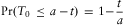$${\rm Pr}\left( {{{T}_0}\,\leq \,a\,{\rm{ - }}\,t} \right)\, = \,{\rm{1 - }}\frac{t}{a}$$

and (by definition)

$${\rm Pr}\left( {T\, = \,t} \right)\, = \,f(t)$$

As usual, calculating the denominator of the Bayes rule (the probability Pr(T + T ₀ ≤ a)) is not crucial as this is only a normalising factorFootnote ³.

We can therefore write

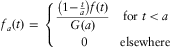$${{f}_a}\left( t \right)\, = \,\left\{ {\matrix{ {\displaystyle\frac{{\left( {{\rm{1 - }}\frac{t}{a}} \right)f\left( t \right)}}{{G\left( a \right)}}} &amp; {{\rm{for}}\ t\,\lt \,a} \cr\ {\rm{0}} &amp; {{\rm{elsewhere}}} \\\end{}} \right$$

Which we can invert to derive an expression for f(t).

$$f\left( t \right)\, = \,\left\{ {\matrix{ {\displaystyle\frac{{G\left( a \right)}}{{\left( {{\rm{1 - }}\frac{t}{a}} \right)}}{{f}_a}\left( t \right)} &amp; {{\rm{for}}\ t\, \lt \,a} \cr\ {{\rm{undefined}}} &amp; {{\rm{elsewhere}}} \\\end{}} \right$$

There is no strictly empirical way of deriving f(t) for t >a. However, if we make some assumption on the way the empirical distribution tails off based on the behaviour for t < a, this derivation becomes possible. This is explored further in Section 2.5.

The non-uniform case. As mentioned above, Equation (16) and all the equations derived from it only hold if it is equally likely that a loss comes from any point inside [0,a]. In actual fact, this will almost never be the case, because of changes in the exposure and in the risk profile. All of this can be captured in the variable v(t) introduced in Section 2.2.1, which we then called the “frequency density”.

Equation (16) can now be rewritten as

$${\rm Pr}\left( {{{T}_{\rm{0}}}\,\leq \,a\,{\rm{ - }}\,t} \right)\, = \,\frac{{\int _{\rm{0}}^{a{\rm{ - }}t} {\rm{\nu }}\left( {{{t}_{\rm{0}}}} \right)d{{t}_{\rm{0}}}}}{{\int _{\rm{0}}^a {\rm{\nu }}\left( {{{t}_{\rm{0}}}} \right)d{{t}_{\rm{0}}}}}\, = \,\mathop \int \sidelimits_{\rm{0}}^{a{\rm{ - }}t} \frac{{{\rm{\nu }}\left( {{{t}_{\rm{0}}}} \right)}}{{\int _{\rm{0}}^a {\rm{\nu }}\left( {t&#x0027;} \right)dt&#x0027;}}d{{t}_{\rm{0}}}\, = \,\mathop \int \sidelimits_{\rm{0}}^{a{\rm{ - }}t} \widetilde{{\rm{\nu }}}\left( {{{t}_{\rm{0}}}} \right)d{{t}_{\rm{0}}}$$

where $$$\widetilde{{\rm{\nu }}}\left( t \right)$$$ is the normalised version of v(t). Equations (18) and (19) can now be amended to take (20) into account.

As a simple but very typical example, consider the case in which the risk profile from one year to the other only changes because of the different exposure (e.g. number of vehicle years for motor insurance, or wageroll/number of employees for employers’ liability). Following the standard (and rough) practice, we'll assume that the exposure undergoes step changes at the beginning of every accident year.

Under these assumptions, it is easy to see that

$${\rm Pr}\left( {{{T}_{\rm{0}}}\,\leq \,a\,{\rm{ - }}\,t} \right)\, = \,\mathop \int \sidelimits_{\rm{0}}^{a{\rm{ - }}t} \widetilde{{\rm{\nu }}}\left( {{{t}_{\rm{0}}}} \right)d{{t}_{\rm{0}}}\, = \,\frac{{\sum _{i\, = \,{\rm{0}}}^{\left\lfloor {a\,{\rm{ - }}\,t} \right\rfloor {\rm{ - 1}}} {{{\epsilon}}_i}\, + \,{{{\epsilon}}_{\left\lfloor {a{\rm{ - }}t} \right\rfloor }}\,\times \,(a\,{\rm{ - }}\,t\,{\rm{ - }}\,\left\lfloor {a\,{\rm{ - }}\,t} \right\rfloor )}}{{\sum _{i\, = \,{\rm{0}}}^{\left\lfloor a \right\rfloor {\rm{ - 1}}} {{{\epsilon}}_i}\, + \,{{{\epsilon}}_{\left\lfloor a \right\rfloor }}\,\times \,(a\,{\rm{ - }}\,\left\lfloor a \right\rfloor )}}$$

where ε_i is the (on-levelled) exposure in year i and $$$\left\lfloor x \right\rfloor $$$ is the integer part of x.

2.3.2 Geometric interpretation

The calculation in Section 3.1 has a simple interpretation in terms of stochastic geometry, as illustrated in Fig. 8. Imagine you have a machine that generates random segments with of length t, where the length of t follows a given distribution f(t), and the segment starts at a point $$${{t}_0}\, \in \,[0,a)$$$ , with an equal probability of starting at any point inside that interval.

Figure 8

A geometric illustration of the probability of observing a delay of length t. Assume we are generating segments of random length t (according to the probability f(t)) with initial point between 0 and a and “letting them fall” – what is the likelihood that they'll make it through the slot? If the length t is given, this probability is simply $$${\rm{1 - }}{t}/{a}$$$ (the length of the segment as a proportion of the length of the slot), which decreases as the length t of the segment increases – and becomes zero when the length of the segment exceeds the length of the slot, because it is impossible for the segment to go through a slot which is smaller than the segment itself. The probability of a segment of random length making it through the slot is instead f_a(t).

The probability of a segment of length t being fully contained inside the slot [0,a) is then

$${\rm Pr}\left( {{\rm{segment}}\,{\rm{is}}\,{\rm{inside}}\,[{\rm{0}},a)} \right)\, = \,\frac{{a{\rm{ - }}t}}{a}\, = \,{\rm{1 - }}\frac{t}{a}$$

and the probability that a segment of random length t is fully contained in the slot is f_a(t) as calculated in Equation (20).

2.4 The case of exponential delays

We have seen in Section 2.2.4 that the expression for the factor to ultimate somewhat simplifies when the underlying distribution f(t) is an exponential distribution with average delay τ:

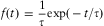$$f\left( t \right)\, = \,\frac{{\rm{1}}}{\tau }{\rm{exp}}(\,{\rm{ - }}\,t/\tau )$$

Using this approximation, the observed distribution in a time window $$$[0,a)$$$ becomes

$${{f}_a}\left( t \right)\, = \,{\frac{{\frac{{\rm{1}}}{\tau }\left( {{\rm{1}}\,{\rm{ - }}\,\frac{t}{a}} \right){\rm{exp}}(\,{\rm{ - }}\,t/\tau )}}{{{\rm{1}}\,{\rm{ - }}\,\frac{\tau }{a}\left( {{\rm{1}}\,{\rm{ - }}\,\exp \left( {{\rm{ - }}\frac{a}{\tau }} \right)} \right)}}$$

and zero elsewhere.

As a consequence, the observed average delay is

$$\matrix {{{{\tau }_{obs}}} &amp; {\, = \,} &amp; {{\Bbb E}(T)\, \,} \cr\ {} &amp; {\, = \,} &amp; {\displaystyle\frac{{\rm{1}}}{{{\rm{1}}\,{\rm{ - }}\,\frac{\tau }{a}\left( {{\rm{1}}\,{\rm{ - }}\,\exp \left( {{\rm{ - }}\frac{a}{\tau }} \right)} \right)}}\mathop \int \sidelimits_{\rm{0}}^a \frac{t}{\tau }\left( {{\rm{1}}\,{\rm{ - }}\,\frac{t}{a}} \right)\exp \left( {{\rm{ - }}\frac{t}{\tau }} \right)dt} \cr\ {} &amp; {\, = \,} &amp; {\tau \left( {{\rm{1}}\, + \,\displaystyle\frac{{{{e}^{{\rm{ - }}\,\frac{a}{\tau }}} \,{\rm{ - }}\,\frac{\tau }{a}\left( {{\rm{1}}\,{\rm{ - }}\,{{e}^{{\rm{ - }}\frac{a}{\tau }}} } \right)}}{{{\rm{1}}\,{\rm{ - }}\,\frac{\tau }{a}\left( {{\rm{1}}\,{\rm{ - }}\,{{e}^{{\rm{ - }}\frac{a}{\tau }}} } \right)}}} \right)} \\\end{}$$

The true underlying average delay can be estimated from Equation (22-iii) by finding τ numerically.

2.5 Calculating the tail factor

Equation (21) shows how to calculate the delay distribution f(t) from the distribution observed through the slot [0,a], f_a(t). However, this prescription works by definition only for delays that are smaller than a. In order to estimate the “tail factor” – i.e., the additional factor by which we have to multiply our projected ultimates in order to take into account delays larger than a – we need to have a prior model for f(t).

If f(t) can be assumed to be an exponential distribution with average mean delay equal to τ, then of course the PDF above a can be modelled as $$$f\left( t \right)\, = \,\frac{{\rm{1}}}{\tau }{\rm{exp}}({\rm{ - }}t/\tau )$$$ . In general, even if f(t) is not an exponential distribution, we can make a broad approximation and do as follows:

1. (i) Calculate the average observed delay τ _obs based on our delay data set

2. (ii) Assume that the delay distribution is exponential and invert Equation (22-iii) to calculate the implied average delay τ

3. (iii) Approximate the delay distribution as

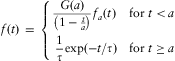$$f\left( t \right)\, = \,\left\{ {\matrix{ {\displaystyle\frac{{G\left( a \right)}}{{\left( {{\rm{1}}\,{\rm{ - }}\,\frac{t}{a}} \right)}}{{f}_a}\left( t \right)} &amp; {{\rm{for}}\ t\, \lt \,a} \cr\ {\displaystyle\frac{{\rm{1}}}{\tau }{\rm{exp}}({\rm{ - }}t/\tau )} &amp; {{\rm{for}}\ t\geq a} \\\end{}} \right$$

Note that in practice this corresponds to a tail factor $$${{\varphi }_{tail}}$$$ given by

$${\varphi }_{tail}}\, = \,\frac{{\rm{1}}}{{{\rm{1}}\,{\rm{ - }}\,{\rm{exp}}({\rm{ - }}a/\tau )}}$$

This is of course a rough approximation, but it gives reasonable results in most cases, unless the tail of the delay distribution has a behaviour which is distinctly not exponential. In any case, there's no reason to get married to this first approximation and if the data are there one can always make a more thorough study of the tail of the distribution by using extreme value theory and finding the parameters of a Generalised Pareto distribution for the tail.

The main risk, as is often the case, is to become a bit too clever and quibble about the exact behaviour of the tail of the delay distribution when there's actually not enough data to support anything more than a simple, one-parameter distribution such as an exponential.

2.6 Other considerations

Non-constant delay distribution. The results above depend on the assumption that the delay distribution f(t) remains constant over time. The method, however, can be easily modified to reflect changes of the delay distribution, e.g. by using a different delay distribution depending on the loss occurrence date. The exact calculations will depend on whether one can consider that the delay depends only on the loss occurrence date (i.e., all losses occurred around a given time have the same average delay) or whether the remaining time to reporting is “accelerated” for all claims from a certain date forwards for all accident years. The key thing is to make sure that one has enough data to support any time-dependency of the delay distribution in order not to introduce spurious accuracy.

Note that the fact that the delay distribution is constant over time is itself a hypothesis that can be easily tested statistically if enough data is available, e.g. by comparing the delay distribution (after the bias correction) before and after a certain time t* for different values of t* with the two-sample Kolmogorov-Smirnov statistic.

Size-dependent delay distribution. In the same way, we can test whether the hypothesis that the delay distribution is the same for claims of all sizes or if, on the contrary, we need a different delay distribution for, e.g., attritional and large losses. We can then apply different IBNR corrections for claims of different size class.

One simple approach in the case that all we need is a distinction between attritional and large losses is as follows:

1. i. Revalue all claims with some measure of claims inflation, to bring them all to current terms

2. ii. Identify the threshold for which the difference in the average mean delay between attritional and large losses is highest

3. iii. Produce a separate delay distribution for attritional and large losses

4. iv. Estimate the number of IBNR attritional losses and IBNR large losses

5. v. Produce a separate severity model for attritional and large losses

6. vi. Produce two different aggregate loss models for attritional and large losses, based on Steps iii to v

7. vii. Combine the two models with a Monte Carlo simulation

The details of how to produce the severity model and how to set up a Monte Carlo simulation will be addressed later on in the paper – at this stage, we just think that it's important to show that a possible dependence of the delay on the size of the loss is not a showstopper. However, we caution against using too many fine distinctions in the case one can't really support them with sound experimental results.

Relationship with claims triangles. As we mentioned before, accident years can be developed individually to ultimate as well as all together. Considering IBNR as a whole leads to a more accurate result, since the development of the more recent years individually to ultimate introduces a large error.

Interestingly, the method can also be used as a complement to the usual claims triangle projection, when the last diagonal is not complete, as a means for grossing up the last diagonal. However, this is perhaps not worth the effort!

3.1 A frequency model for IBNR losses

In this paper we will assume that the underlying frequency distribution is either a Poisson distribution or a negative binomial distribution.

The Poisson distribution has its theoretical justification as the natural model for rare independent events arising from a stationary process. In the presence of systemic volatility, clustering of claims or simply parameter uncertainty, the dispersion of the Poisson distribution (for which the variance-to-mean ratio is 1) may not be sufficient to reproduce reality. The negative binomial distribution is simply one way to account for this additional dispersion, and there is nothing fundamental about this distribution – it's just that it can be easily represented as a Poisson distribution whose Poisson rate is itself a random variable drawn from a Gamma distribution. It is very seldom the case that one has such a wealth of experimental data that the use of the negative binomial can be challenged!

The Poisson case

Under the Poisson assumption, the IBNR claim count can be represented as a Poisson distribution for which:

• • The Poisson rate is the point estimate of the IBNR claim count, as calculated by Equation (5) (or Equation (6) for the discrete case);

• • The standard error on the Poisson rate can be approximated as the square root of the Poisson rate itself (as this is the best estimate of how much variation we expect from one simulation to the other).

Note that although the process is assumed to be Poisson, when we use this frequency distribution later on for Monte Carlo simulation, we will need to take the parameter uncertainty into account and this will be equivalent to having an overdispersed Poisson distribution: specifically, we will use the negative binomial approximation by assuming a variance-to-mean ratio of 2 (as in this case the process variance is equal to the parameter uncertainty).

The negative binomial case

Under the negative binomial assumption, the IBNR claim count can be represented as a NB distribution for which:

• • The rate is the point estimate of the IBNR claim count, as calculated by Equation (4) (or Equation (6) for the discrete case);

• • The variance-to-mean ratio can be estimated by calculating the projected number of claims for different years, as in the “Ultimate losses” column of Fig. 7, calculating the variance based on those ultimate lossesFootnote ⁴, and dividing it by the average of the ultimate losses;

• • The effective variance-to-mean ratio can then be derived from the variance-to-mean ratio by adding an allowance for the parameter uncertainty as in the Poisson case. As a simple rule of thumb (using a rough application of the central limit theorem), the effective variance-to-mean ratio can be written as $$${{(V/M)}_{\rm eff}}\, = \,(V/M)\, + \,{\rm{1}}/n$$$ where n is the number of years over which the variance was calculated. (It can be seen that in the case of Poisson this gives back the “variance-to-mean ratio=2” rule stated for the Poisson case.)

3.2 A severity model for IBNR losses

We now need to produce a severity model for IBNR claims, with the ultimate goal of producing an aggregate loss distribution for IBNR claims via Monte Carlo simulation. Since one of the things that we'll need to simulate will be the actual occurrence date for the claims, the distribution from which we sample the random loss amounts will in general be different depending on the occurrence date. This dependency is analysed in Section 4.1.

Another thing we need to take into account is IBNER, which is dealt with in Section 4.2.

Once we take these two elements into account, we'll have a way of sampling the severity of claims. The algorithm is illustrated in Section 4.3.

3.2.1 Dependency of the loss distribution of IBNR claims on the occurrence date

As in experience rating, the main difficulty in obtaining a severity model is that IBNR claims will come from different years of experience, and each accident year may well have a different severity distribution, depending on the specific business mix that was written in that particular yearFootnote ⁵.

There are at least two different elements that drive the dependency of the severity distribution on the accident year.

• • The proportion of different types of claims may change, as a result of changing business conditions or simply the changing nature of risk due to environmental/technological changes (e.g., the relative number of “slips and trips” public liability claims might be increasing due to a more litigious environment, or decreasing due to better risk control mechanisms such as anti-slippery carpets)

• • Claims inflation – losses occurring now will generally have a different cost (usually higher) than losses occurred a number of years ago. Furthermore, the severity distribution of losses that have not been reported yet might also be conditional on the reporting delay: e.g., losses that have occurred five years ago and were reported then might not follow the same distribution as losses that have occurred five years ago and are reported today. (It is not obvious whether they will be bigger or smaller – one can argue that a menial loss will either be reported immediately or not be reported at all, but might also argue that if a loss is really big it will be more evident and will certainly be reported shortly. Only empirical evidence can help us make an informed stance.)

In the following, we will focus on claims inflation and ignore changes coming from changes in business mix or in the type of claims: if this is not the case, we always have the option of splitting the loss experience into claims of different type and analyse them independently, assuming that the severity distribution within each segment remains the same except for claims inflation.

So how do we take claims inflation into account? In experience rating what one normally does is to analyse the past experience over a period and revalue to current terms (or rather, to the mid-term of the policy one wishes to rate) all past claims by a certain index (e.g. a wage inflation index, perhaps amended to include extra inflation) or a flat inflation rate which is assumed to incorporate all necessary elements of inflation.

In determining the severity model for IBNR losses, we need to go through a similar process, with the complication explained above and repeated here more formally: we are interested in the probability $$$F_{X}^{{{{t}_0},\delta }} \left( x \right)$$$ that a loss X be ≤ x conditional to X having occurred at time t ₀(assume the time is given in years) and being reported after δ years.

$$F_{X}^{{{{t}_0},\delta }} \left( x \right)\, = \,{\rm{{\rm Pr}}}(X\,\leq \,x,X\,{\rm{occurred}}\ {\rm{at}}\ {\rm{}}{{t}_{\rm{0}}}{\rm{,}}\ {\rm{reported}}\ {\rm{at}}\ {{t}_{\rm{0}}}\, + \,\delta )$$

There are therefore two (possibly conflicting) effects: that of claims inflation and that of being reported after a number of years.

Ultimately, only empirical evidence helps tell us what this distribution looks like. One approximation that we can often use is to assume that $$$F_{X}^{{{{t}_0},\delta }} \left( x \right)\left( x \right)$$$ is simply a scaled version of the kernel distribution F(x), where the scaling depends on both the year of occurrence and the reporting delay:

$$F_{X}^{{{{t}_0},\delta }} \left( x \right)\, = \,{{F}_X}\left( {\frac{{{{{({\rm{1}}\, + \,r)}}^{t{\rm{ - }}{{t}_{\rm{0}}}}} x}}{{{{{({\rm{1}}\, + \,s)}}^\delta } }}} \right)$$

where t is the current time, r is the claims inflation (assumed constant here for simplicity), and s is an inflation that captures the effect of the reporting delay: e.g., if claims tend to become larger when δ increases, then s > 0 . Vice versa, it is <0.

This is just a rough working assumption, but it is often a good approximation of reality, as it is shown for example in Fig. 9, which shows the empirical distribution of employers’ liability losses for a large UK company for the same accident year (2006) and different reporting years (2006, 2007, 2008 and later). Even without any delay-related inflation (i.e., assuming s = 0 in Equation (22-vii)), we see that the empirical distributions are quite close, e.g. there is no obvious effect on the severity distribution due to reporting delay.

Figure 9

The graph shows the empirical distribution of employer's liability losses for a large UK company in the food services industry, after some scaling to make the losses unrecognisable. The empirical distributions for 2006 losses that have been reported in 2006, 2007 and 2008 or later have been compared, without adding any delay-related inflation. The empirical distributions are visually very similar, and this is confirmed by the Kolmogorov-Smirnov statistical test: the normalised KS distance between the differen pairs is KS(RY = 2006, RY = 2007) = 1.22 (p = 10%), KS(RY = 2006, RY = 2008+) = 1.36 (p = 5%), KS(RY = 2007, RY = 2008+) = 0.74 (p >> 10%).

A rough approximation may therefore be to simply ignore delay inflation and set r equal to a standard claims inflation rate for the line of business under consideration: e.g. r = 5% s = 0.

The situation needs of course to be assessed on a case-by-case basis and ultimately only empirical evidence can lead us one way or another – the important thing to remember as usual is that models that are more sophisticated than Equation (22-vii) need to be supported by a proportionate wealth of empirical evidence.

3.2.2 Determining IBNER in order to derive the severity distribution

Many of the losses that make up the loss data set and that we need to use to derive the severity distribution are still outstanding (not paid up) and as such are still liable to change in value. This is a type of data uncertainty which we denote generically as “IBNER” (incurred but not enough reserved/reported). IBNER has an impact on both the selection and the parameterisation of the severity distribution.

The idea of IBNER analysis is to identify systematic underestimation or overestimation of claims and to put it right by adding the relevant (possibly negative) amount to all open claims.

For large losses (and especially in reinsurance), this is normally done by using an individual claims development table which is made of triplets of rows like that in Fig. 10.

Figure 10

The history of a claim occurred in 2000 and reported in the same year. For each year of development, the paid, outstanding and incurred (estimated) amounts are given. The outstanding ratio (outstanding amount divided by incurred amount) is also given for each year. The last row shows the IBNER factors for this claim, calculated as the ratio between the incurred amounts of two successive years. The claim shown here is a real claim after scaling by a random amount and the removal of any identifiable information (Figure borrowed from Parodi (Reference Parodi2012a)).

The calculation of the IBNER factors between two successive years of development of the claims is usually performed by an average (weighted or unweighted) over all open claims (settled claims will of course have no IBNER, unless they are re-opened) as in Fig. 11.

Figure 11

Claims listing in a format suitable for IBNER calculation. The claims are actual anonymised general liability claims from a single large company (only the first three years of development of only the first few claims are shown). The IBNER factor, e.g., from year 1 to year 2 is calculated as a weighted average of the individual IBNER factors of non-zero claims that are still outstanding (settled claims obviously have no IBNER) from year 1 to 2: IBNER(1 −>2) =(1,535,000 + 85,960 +⋯)/(2,486,700 + 116,660 +⋯). If the data is abundant it is also possible to measure the volatility of this IBNER factor and the distribution around the mean value.

If the data is abundant, it is also possible to estimate the volatility of the IBNER factors around the mean value and actually the whole distribution of the IBNER factors, as in Fig. 12.

Figure 12

The distribution of the IBNER factors from development year 1 to development year 2, based on the data set whose first few rows are shown is Fig. 11. Note that the largest factors (>2) have been removed for legibility's sake. Also note the peak at 1, showing that many claims did not change their value from the first to the second year of development.

A more refined analysis

The simple method described above focuses on the dependence of the IBNER factor from the year of development, be it from the loss year or from the reporting year. However, it is obvious that the IBNER factor will depend in general on many factors, such as:

• • development year d (the younger the claim, the more scope there is for it to deviate from the incurred estimate), as already mentioned;

• • size of claim x (larger claims may have more uncertainty about them);

• • outstanding ratio r (the larger the outstanding amount, the more conjectural the estimate of the incurred value will be);

• • type of claim t (for example, bodily injury claims will be more difficult than property claims to estimate reliably as the victim's health may worsen unexpectedly);

• • …

As in all situations in which one needs to understand how different factors impact a given variable, this is a problem of statistical learning (see for example Parodi (Reference Parodi2012a), where the problem of IBNER analysis was specifically addressed as an example). A typical technique used in insurance to solve statistical learning problems is generalised linear modelling. According to this approach, we can write IBNER factors as a linear combination of different variables, possibly further transformed by a function h:

$$IBNER(d,x,r,t \ldots )\, = \,h({{a}_1}{{f}_1}(d,x,r,t \ldots )\, + \, \cdots \, + \,{{a}_n}{{f}_n}\,(d,x,r,t \ldots ))$$

and identify the relevant functional form of h, f ₁,… f_n and the parameters a ₁,…a_n that are suitable to describe the IBNER factors. For example, one might consider a very simple model such as

$$IBNER\left( {d,x,r} \right)\, = \,{{e}^{{\rm{ - }}({{a}_{\rm{1}}}\, + \,{{a}_{\rm{2}}}d + {{a}_{\rm{3}}}x\, + \,{{a}_{\rm{4}}}r)}} $$

which is a special case of the more general Eq. (24), where f ₁(d, x, r, t, s …) = 1, f ₂ (d, x, r, t, s …) = d, f ₃(d, x, r, t, s …) = x, f ₄(d, x, r, t, s …) = r, h(x) = exp (x).

Output of the IBNER analysis

As a result of this GLM analysis – or even if we use the simple approach outlined at the beginning of this section – we will have:

1. a. The IBNER factors to project each existing claim to ultimate. We can then use the projected values of the outstanding claims along with the settled claims to derive the severity distribution

2. b. A distribution of values around each IBNER factor, which will allow us to consider each outstanding claim not as a point estimate but as a distribution of possible ultimate values

Note that the fact that there is uncertainty around the ultimate value of each claim, as captured by the distribution in Point (b) above, has the consequence of increasing the parameter uncertainty on the parameters of the severity distribution, as discussed for example in Parodi (Reference Parodi2012a).

Note, finally, that there is no theoretical reason why we need to separate the claims estimates into accident years, as if claim reserves only could be revised at regular intervals, so the variable d in the equations above may be a continuous as well as a discrete variable.

Practicalities

In practice, the historical development of each claim may not be available, especially for small claims, in which case other solutions must be used:

• • If we have at least an initial estimate for the claim and then the final settlement value, we can use those to estimate IBNER;

• • If we only have the information on whether a claim is open or closed, we may want to check whether the distribution of the open and closed claims are close enough (in terms, e.g., of the Kolmogorov-Smirnov distance) and if not, we may want to only consider closed claims to derive the severity distribution. However, this is often dangerous and risks underestimating the average loss severity a great deal as large losses often take much longer to settle and therefore they may be hugely underrepresented. This method should be used only if most claims are settled quickly, and making sure that no significant bias is introduced;

• • In some cases we may have both a database of individual losses with little or no information on the history of claim reserves, but we may be given a pre-cooked claims triangle (which is sometimes the only input used for reserving studies) with both the non-zero claim count and the aggregate losses. In this case we can derive a triangle for the average claim amount and from that derive a rough measure of IBNER, which we can then use to modify the individual claim amounts. This is a hybrid method which is unlikely to be satisfactory but it may be better than ignoring IBNER altogether.

• • If we have no information at all which is relevant to IBNER, that is, we have no average claim triangles and we do not even know which claims are open and which are closed, then as a first approximation we'll simply need to assume that there is no IBNER, or use industry IBNER factors. E.g., in the US market IBNER factors are provided by institutions such as the NCCI and the ISO for different classes of business (e.g. workers’ compensation, auto liability), by territory and by type of risk.

3.2.3 Overall algorithm to create a severity model for IBNR claims

Now that we have methods for revaluing IBNR claims (Section 4.1) and to adjust for IBNER (Section 4.2) we can put the pieces together and produce a severity model for IBNR claims. This is a bit different from what one does in pricing.

In the case of pricing, all we need is the severity distribution for the policy we wish to price. The severity model is simply a statistical distribution F_X(x) that gives the probability that a given loss X has a value less than or equal to x: $$${{F}_X}\left( x \right)\, = \,{\rm Pr}\left( {X\,\leq \,x} \right)$$$ . This can be estimated empirically by fitting a suitable statistical distribution to the past losses after they're revalued and adjusted for IBNER.

The severity model for IBNR claims will need to be a slightly more complicated object, as we will need to take into account the fact that the size of the claim will also depend on when the claim occurred. What we need is therefore the probability that a loss X is less than or equal to x conditional on the fact that the loss has occurred at time t _occ and has not been reported by the as-at date (t _as-at):

$$F_{X}^{{IBNR}} \left( {x,{{t}_{{\rm{occ}}}},{{t}_{{\rm{as}}\,{\rm{ \hbox{-} }}\,{\rm{at}}}}} \right)\, = \,{\rm Pr}\left( {X\,\leq \,x&#x007C;{{T}_{{\rm{occ}}}}\, = \,{{t}_{{\rm{occ}}}},{{T}_{{\rm{rep}}}}\,\geq \,{{t}_{{\rm{as}}\,{\rm{ \hbox{-} }}\,{\rm{at}}}}} \right)$$

A possible algorithm to create a severity model for losses X occurring at time t _occ and not yet reported as at t _as-at is as follows:

Input. The inputs to the severity analysis are the individual claim amounts (both paid and estimated)

1. 1. Adjust individual past losses for IBNER, as in Section 3.2.2.

2. 2. Revalue the individual past losses to current terms with some agreed index/inflation rate

   • • This we need to do so as to determine the joint underlying severity distribution from all years, as if all losses were to occur today

3. 3. Model the severity distribution in current terms, according to standard methods (e.g. a lognormal distribution plus separate tail modelling), obtaining what we will refer to as the kernel severity distribution (since this is the nucleus from which the distribution for the different years will be constructed through transformations).

4. 4. Estimate the severity distribution for losses that occurred at time t _occ and that have not yet been reported by transforming the kernel severity distribution according to the method explained in Section 3.2.1 (perhaps using the approximation that there is no delay inflation), or any alternative valid method.

The algorithm outlined in Steps 1 to 4 (and which simply collects all observations dealt with in Sections 3.2.1 and 3.2.2) gives the theoretical background for the severity model of IBNR losses. In Section 3.3 we will see how we can actually sample from the IBNR distribution.

3.3 A protocol for simulating IBNR losses

Now that we have a frequency model and a severity model, we can combine them in the spirit of the collective risk model to produce an aggregate loss distribution. This can be done, e.g., by a Monte Carlo simulation.

We need a “simulation protocol” which takes all the subtleties of the IBNR distribution into account: we need to determine not only how many losses there will be in each simulated scenario, but also when each of these losses is assumed to have occurred, and from what severity distribution we need to sample.

There are many ways in which we can do this, but as an illustration we are going to use a property of the Poisson distribution – assuming, for now, that the Poisson rate is uniform over the years (i.e., the variable v(t) in Section 2.2.1 is constant): an assumption we'll drop shortly.

If we subdivide the period from which the losses are assumed to originate (normally there will be some constraint on how far back we can go) into small intervals (t′, t′ + Δt) of length Δt, we can assume that the number of losses in each of these small intervals is either 1 or 0 (see, e.g., Ross, Reference Ross2003), and that it is 1 with probability $$$\lambda ({\rm{1 \,- }}\,F\left( {t\,{\rm{ - }}\,t&#x0027;} \right))\,{\rm{\Delta }}t$$$ , where F (t − t′) is the probability that a loss from the interval (t′, t′ + Δt) has been reported by time t (see Section 2).

This has a simple geometric interpretation: it is exactly like drawing a number (distributed as a Poisson variate with rate equal to the point estimate of the IBNR claim count over the years) of random dots uniformly from inside the dark green area of Fig. 6 (which we reproduce here for convenience), and select the x-coordinate as the simulated time of occurrence.

In the general case, the Poisson rate is not uniform, and the process may actually be a negative binomial process). Let's deal with these two aspects in turn.

Non-uniformity. The geometric interpretation above is still valid if the Poisson rate is not uniform, but the geometric figure must be warped a bit: instead of the rectangle representing the expected ultimate claims as in Fig. 6 we have to consider the area below the function v(t′), and instead of the light-green area in Fig. 6 giving the expected reported we have the area below the function v(t′) F(t−t′).

Negative binomial case. In case a negative binomial distribution process is used as a model for the IBNR loss count (even if only to represent the parameter uncertainty for the Poisson case), we can simply draw the number of IBNR losses from a negative binomial distribution by using the familiar Poisson/Gamma mixture process, and then sample it in proportion to v(t′) (1−F(t−t′)). The problem with this method is that it does not reproduce the extra year-on-year volatility which is typical of realistic loss processes. This is a known problem: “sample realizations of such processes look [like] Poisson ones – the variation is not within, but between processes” (Kozubowski & Podgorski, Reference Kozubowski and Podgorski2009). If we want to reproduce this extra volatility, we need to use another realisation of the NB process, e.g. the Poisson/Logarithmic mixture process, which creates clusters (“colonies”) of losses happening at the same time (ibid.). If we use this framework, it is these “colonies” of losses that are distributed at random in the dark-green area of Fig. 6.

Based on the considerations above, we outline the following protocol for simulating IBNR losses.

Simulation protocol

Input: Rate of IBNR losses, λ, effective variance-to-mean ratio (the one which includes the parameter uncertainty), 1 + R, and the kernel severity distributionFootnote ⁶, F_X(x).

1. i. For each scenario j = 1 to N _sim, simulate the number n_j. of IBNR claims from a negative binomial distribution with rate = λ and variance-to-mean ratio = 1 + R.

2. ii. For each loss i = 1 to n_j, simulate the loss occurrence date as described above, in proportion to v(t′) (1−F(t−t′)), where t′ is the occurrence date and t is the as-at date

3. iii. For each loss i = 1 to n_j, if t_j is the loss occurrence date, sample a loss $$$x_{i}^{{(j)}} $$$ from the kernel loss distribution F_X(x), then modify it to take into account the loss occurrence date, e.g. (using Alternative Assumption 1 in Section 3.2.1) $$${x&#x0027;}_{i}^{(j)} \, = \,{{({\rm{1}}\,{\rm{ + }}\,r)}^{{{t}_j}{\rm{ - }}t}} x_{i}^{{(j)}} $$$ .

4. iv. Loop over i

5. v. Calculate the total losses for each scenario j, as $$${{S}_j}\, = \,\mathop \sum \limits_{i\, = \,1}^{{{n}_j}} x_{i}^{{(j)}}$$$

6. vi. Sort all values of S_j in ascending order: $$${{S}_{\left( {\rm{1}} \right)}}\, \lt \,{{S}_{\left( {\rm{2}} \right)}}\, \lt \, \cdots \, \lt \,{{S}_{\left( {{{N}_{{\rm{sim}}}}} \right)}}$$$

Output: The empirical aggregate loss distribution, $$${{\widehat{F}}_S}\left( s \right)\, = \,\max \left\{ {j&#x007C;{{S}_{\left( j \right)}}\,\leq \,s} \right\}/{{N}_{{\rm{sim}}}}$$$ .

6.1 Dependence among IBNR, RBNS and UPR

How good is the assumption that the IBNR, RBNS and UPR distributions are independent?

Conditional to the risk model which has been derived for each of these components (and involving, where applicable, a reporting delay distribution, a frequency distribution and a severity distribution) being correct, there is no residual dependency between the three components.

For example, the number of IBNR claims that will actually be reported in practice is – again if our frequency model is correct – independent of the number of claims that will be reported for the unearned portion of the premium (UPR), i.e. the future losses, much in the same way that the number of losses occurred in one year is independent of the number of losses occurred in another year, although the underlying frequency may be the same.

The same is true for our severity distribution and our reporting delay distribution – if we're sampling from the same severity distribution, subject to all the modifications discussed in Section 3.2.1, the actual samples for IBNR and UPR will be independent.

And that is also true for RBNS. You will have noticed that the modelling decisions one makes for RBNS have an impact on IBNR, RBNS and UPR, at least if open claims are used to produce the kernel severity distribution. However, if the model you have produced for RBNS is correct, the IBNER amount that you need to add to a particular claim to obtain the claim's ultimate true value is independent of the IBNER amount that you need for another claim, whether it's not occurred yet, incurred but not reported, or reported but yet outstanding.

However, that does not mean that we can ignore dependency under all circumstances. There are at least two types of dependency that we may want, or even need, to take into account.

1. 1. Modelling choices. These are the correlations that arise out of the modelling process itself. The severity model that we use for UPR and IBNR is based on the same kernel severity model, and therefore any parameter and model choice that we make will affect both estimates. E.g., if we choose a lognormal model for both UPR and IBNR but the true model turns out to be a Gamma distribution, this wrong choice will affect both UPR and IBNR in the same way. So the correlation is not in the loss process but is an artifact of the calculation method.

   How do we deal with this? Correlations arising out of the modelling process can be easily taken into account by making sure that the modelling choices (e.g. the parameters) are the same across the different components (RBNS, IBNR, UPR) of a given simulated scenario. The output of the simulation will therefore reproduce these correlations.

2. 2. Systemic shocks. These are the correlation that are created by the fact that some of the assumptions behind the model need to be changed. An example is if the discount rate applied by the courts to produce an estimated lump sum for liability claims – if it were changed to reflect, say, lower returns on gilts, all claims that are not settled (whether reported but outstanding, incurred but not reported, or not incurred yet) might be affected and that would mean that the IBNER, IBNR and UPR distributions would change. On the frequency side, a change in legislation that encourages or discourages the reporting of claims will have an impact on both UPR and IBNR claims (not on RBNS, since the number of outstanding claims is fixed).

   How do we deal with this? Correlations arising out of systemic shocks can be modelled by using a so-called correlation shock. Assume, for example, that we have convinced ourselves that the discount rate will go down by 0.5% with a probability of 1/50, and by 1% with probability of 1/100 (the probability of remaining the same being therefore 97/100). We then assess the effect of this discount rate change on the severity distribution, and as a consequence on all UPR, IBNR and RBNS. Finally, for each simulation scenario we choose at random one of the three situations (constante discount rate, 0.5% decrease, 1% decrease) with the relevant probabilities, and we apply the same assumption across all the three components of the simulation (UPR, IBNR, RBNS).

7.1 Producing the frequency model

7.1.1 Estimating the report delay distribution

We have estimated the report delay distribution, based on the observed empirical delays. The adjustment for the bias introduced by the limited observation window has been carried out as explained in Section 2. We have not assumed a specific model (e.g. exponential) for the delay distribution. The bias-corrected empirical delay distribution is shown in Fig. 13.

Figure 13

The empirical reporting delay distribution, after correction for the bias introduced because of a limited observation window.

7.1.2 Counting the number of non-zero reported losses

We have then counted the number of non-zero reported losses for each accident year.

We had to take into account the fact that some of the losses reserved as non-zero may end up being zero (especially, and almost exclusively, if they're 100% outstanding). There are several ways to do this. When we have the historical loss amount for each loss, as in this case, we can calculate the percentage of non-zero, 100% outstanding claims that drop to zero for each year of development, and based on that we can estimate the number of currently reported claims that will end up being zero. This is illustrated in Fig. 14.

Figure 14

Based on the historical individual loss information (that information that we have also used to analyse IBNER) we have calculated the probability that a claim drops to zero after being reported. E.g., there is a 4.6% that a claim which is non-zero in development year 0 will drop to zero in development year 1 – or, in other terms, there is a 95.4% probability that the claim will not drop to zero (what we call in the table the survival probability. Overall, the cumulative survival probability that a claim which is non-zero in development year 0 will eventually drop to zero is 100%–79.1% = 20.9%.

Armed with the statistics shown in Fig. 14, we can count the number of claims that are fully outstanding for each year and from that we can determine the number of non-zero losses expected to survive, as illustrated in Fig. 15. This will be the input to calculate the projected number of claims for each year.

Figure 15

Each of the fully outstanding losses (column 4) has a survival probability that depends on its year of development. Summing all these survival probabilities for each claim occurred in a given year we can find the number of losses that are fully outstanding and that are expected to survive indefinitely (column 5). The number of non-zero losses expected to survive (column 6) is given by the number of non-zero reported losses (column 3)+the number of fully outstanding losses expected to survive (column 5) – the number of fully outstanding losses (column 4).

7.1.3 Estimating the IBNR/UPR claim count

We can now use the reporting delay distribution (Fig. 13) and the claim count (Fig. 15, column 6) to project the claim count to ultimate for each year, or on aggregate and produce a frequency model.

We have used a negative binomial to model the claim count. This is defined by two parameters: the mean claim count and the variance-to-mean ratio, which can be calculated by projecting each year independently and then calculating the year-on-year variance, as in Fig. 16.

Figure 16

This chart shows the claim count (grey line) for each year after adjustment for exposure changes (light blue bars), the projected claim count for each year (blue line, with error bars of size equal to twice the standard error), and the estimated mean claim count (30.2) at an arbitrary level of exposure (dashed red line), calculated as a weighted average of years 2001–2010 (2011 is too immature). (Note: The arbitrary level of exposure was in this case chosen to be the estimated next year's exposure (515 arbitrary units): this makes sense in a pricing context but in this case all it matters is the frequency per unit of exposure.)

The estimated parameters of our frequency model are a mean of 0.0586 claims per unit of exposure and a variance-to-mean ratio of 1.25 (which also takes into account parameter uncertainty).

Once we have an estimate of the frequency model per unit of exposure, we can estimate the projected IBNR amount for each year at the relevant exposure. The variance-to-mean ratio plays a role in the calculation of the standard error with which the projected IBNR amount is known.

The IBNR calculations on an unadjusted basis (i.e., no corrections for changes in exposure) are shown in Fig. 17 (chart form) and Fig. 18 (tabular form).

Figure 17

Projection of claim count (grey line) to ultimate (blue line) for each year, without adjustments for exposure changes (light blue bars).

Figure 18

The first nine columns show the same information as the chart in Fig. 17 but in tabular format. The input data (latest reported, exposure) is indicated in blue; the intermediate calculations are in black; the outputs we're interested in are in purple. The last four columns illustrate the credibility calculations that lead to a revised figure for IBNR, which is very similar to the one based on client data only for all years except for 2011.

Note that the 2011 projected figures include both IBNR and UPR.

The IBNR calculations illustrated in Fig. 17 and Fig. 18 are performed year by year. As a consequence, the projection of the last few years get increasingly more uncertain, as they're based on an increasingly smaller number of claims. This is especially true for 2011, which is strongly underdeveloped.

This problem is not specific to triangle-free reserving – exactly the same phenomenon happens with the chain ladder and with every attempt to project losses to ultimate based on last year's data alone.

A more accurate estimate of the overall number of IBNR claims can be obtained by lumping all years together, as shown in Fig. 19.

Figure 19

The same calculations as in Fig. 18, but without artificially splitting the estimate by year.

Another possible solution to the problem of having unstable results for the most recent year(s) is to adopt a credibility approach. This is not very different from what we do with Bornhuetter-Ferguson and Cape Cod for triangulation methods.

In order to produce a credibility-weighted estimate for all years, we need a benchmark against which to compare the raw projections. A natural benchmark is provided by the estimated number of claims for each year based on the frequency per unit of exposure derived above ( $$$\widehat{\lambda }\, = \,{\rm{0}}{\rm{.0586}}$$$ ) and the exposure for each year, $$${\rm{{\epsilon}}}(y)$$$ :

$${\rm{Projecte}}{{{\rm{d}}}_b}(y) = \widehat{\lambda }{\rm{{\epsilon}}}(y)$$

The volatility of such a figure will be given by the projected amount times the variance-to-mean ratio, yielding:

$${\rm{Var\_Projecte}}{{{\rm{d}}}_b}(y)\, = \,({\rm{1}}\,{\rm{ + }}\,r)\widehat{\lambda }{\rm{{\epsilon}}}(y)$$

This credibility factor can then be calculated by balancing this prior volatility against the standard error (squared) on the projected ultimate for each year (see, e.g., Parodi & Bonche (Reference Parodi and Bonche2010)). This standard error is calculated according to Equation (11) and leads to the numbers in Fig. 18 (C6). The credibility factor for year y is then given by:

$$Z(y)\, = \,\frac{{{\rm{Var\_Projecte}}{{{\rm{d}}}_b}(y)}}{{{{{\left( {{\rm{s}}{\rm{.e}}.(y)} \right)}}^{\rm{2}}} \, + \,{\rm{Var}}\_{\rm{Projecte}}{{{\rm{d}}}_b}(y)}}$$

(Note that since the variance-to-mean ratio is included in all terms, in practice it plays no role in Equation (27c).)

The credibility estimate is thus given by

$${\rm{Cred\_Estim}}\left( y \right)\, = \,Z\left( y \right){\rm{Ult}}\left( y \right) + ({\rm{1 - }}Z\left( y \right))\widehat{\lambda }{\rm{{\epsilon}}}(y)$$

Which in terms of the columns of Fig. 18 can be written as $$${\rm{C16}}\,{\rm{ = }}\,{\rm{C15}}\,{\rm{\times }}\,{\rm{C5}}\,{\rm{ + }}\,{\rm{(1 - C15)}}\,{\rm{\times }}\,{\rm{C13}}$$$ .

The credibility estimate for IBNR can then be calculated by applying the IBNR percentage (column C12) to the credibility estimate for the ultimate of Eq. (27d), leading to the results of column C17.

7.2 Producing a severity model

7.2.1 Adjusting for IBNER

We do a simple IBNER calculation based on the average of past IBNER factors by development year. This was done as explained in Section 3.2.2. The results are shown in Fig. 20.

Figure 20

Average IBNER factors for our data set. IBNER factors are assumed to be 1 after year 4 because the dwindling sample size makes it difficult to have confidence in the estimate.

The cumulative IBNER factors of Fig. 20 (column 3) are then applied to all open claims (open = more than 5% outstanding) of the relevant year of development in order to estimate the final settled amount.

7.2.2 Is there a common severity model to all years?

In its simplest form, our approach assumes that the severity distribution is the same for all years, except for claims inflation and possibly for the dependency of the average size on reporting delay. In this section we are going to test this assumption.

First of all, we revalue all claims by 5% p.a. (a common assumption for liability claims) to 2011, and we adjust all RBNS claims by the appropriate IBNER factor as derived in Section 7.2.1.

We then compare the empirical severity distribution of different years. To have samples that are statistically more significant, we have grouped years in sets of three: 2001–03, 2004–06, 2007–09, 2010–11 (this last set only has roughly 1.5 years).

Fig. 21 shows that the assumption that there is a common severity distribution to all years (except for claims inflation) is a good one for this risk. This can be appreciated visually but can also be confirmed statistically by looking at the two-sample KS distance among the different sets (Fig. 22).

Figure 21

A comparison of the empirical severity between different years. Note that the comparison has been performed after adjusting for IBNER. Since the IBNER factors are spurious in this case (IBNER factors of data set (b) have been applied to data set (a)) it is likely that the differences between the years have been exaggerated.

Figure 22

A statistical comparison among the data sets. All sets can be considered as coming from the same distribution with a significance level of 10% (remember that the normalised KS distance at a confidence level of 10% is 1.22).

7.2.3 The kernel severity model

We then bring all the revalued losses together and build a kernel severity model from which the model for the different years can be derived. We have modelled the losses with an empirical distribution (i.e., resampling of existing losses) up to £10,000 and then a GPD with parameters ξ = 0.736, σ = 18,263, μ = £10,000 above that (Fig. 23).

Figure 23

Severity model (blue line) vs revalued and IBNER-adjusted losses (red dots). Note that the empirical distribution was used below £10,000 (hence the perfect fit below that threshold).

7.3 The aggregate model for IBNR/UPR losses

We can now combine the frequency model (Section 7.1) and the severity model (Section 7.2) for IBNR/UPR losses with Monte Carlo simulation. We can use a separate model for each year (which is the option we've adopted here) or we can combine all years in a single one by mixing the severity distributions in proportion to the frequency of IBNR claims.

(Note that we have used for the IBNR frequency the projection year by year based on column C11 of Fig. 18, not the credibility estimate – this is not because we believe this estimate is better but simply because we had to choose one of the cases for illustration purposes.)

Fig. 24 shows the output of this exercise.

Figure 24

The output of the Monte Carlo simulation for each year of occurrence, and with all years combined.

7.4 The aggregate loss model for RBNS losses

In order to analyse the distribution of possible outcomes for RBNS losses, let us first look at the settlement pattern for open claims. Fig. 25 shows empirical statistics for our data set. These are obtained by looking at the percentage of claims of “age” (development year) d that have already been settled, and deriving from that the conditional probability that a claim which has already reached age d will be settled by the time it reaches age d’.

Figure 25

This table gives the probability that a claim settles at year s conditional to the fact that is still outstanding at development year d. For the purpose of this exercise, “settled” means that less than 5% of the overall estimated amount is still to be paid. (The reason why this is considered settled is that often after the indemnity part of a claim has been paid, the insurer might still incur relatively minor expenses.)

Given the crucial information of Fig. 25, we can now produce a distribution of possible outcomes for RBNS claims according to one of the methods mentioned in Section 4. In this specific case, we have adopted the following algorithm, which is a specific version of the general algorithm described in Section 4.

Input: All the open losses with their year of development, and all the IBNER factors model

1. (i) For each scenario j = 1 to N _sim

   1. a. For each open loss X_k

      1. i. sample a value of the settlement year s(j, k), based on the past stats for settlement time (see Fig. 25);

      2. ii. sample IBNER factors $$${\rm{IBNE}}{{{\rm{R}}}_{d,d\, + \,1}},{\rm{IBNE}}{{{\rm{R}}}_{d +, d\, + \,2}} \ldots {\rm{IBNE}}{{{\rm{R}}}_{s\left( {j,k} \right){\rm{ - }}1,s(j,k)}}$$$ from the empirical distribution (i.e. the actual IBNER factors)

      3. iii. calculate the cumulative IBNER factor for this loss by multiplying these factors together: $$${\rm{IBNER}}_{k}^{j} \, = \,{\rm{IBNE}}{{{\rm{R}}}_{d,d\, + \,{\rm{1}}}}\,\times \,{\rm{IBNE}}{{{\rm{R}}}_{d +, d\, + \,{\rm{2}}}}\,\times \, \cdots \,\times \,{\rm{IBNE}}{{{\rm{R}}}_{s\left( {j,k} \right){\rm{ - 1}},s(j,k)}}$$$ ;

      4. iv calculate the IBNER-adjusted value of the claim, $$$X{{&#x0027;}_k}\, = \,IBNER_{k}^{j} \,\times \,{{X}_k}$$$

   2. b. Sum over all IBNER-adjusted claims, obtaining the simulated ultimate RBNS for simulation j: $$$S_{{}}^{j} \, = \,\mathop \sum \nolimits_{k\, = \,1}^n X{{&#x0027;}_k}$$$

2. (ii) Repeat for all scenarios

3. (iii) Sort all the values S ^j, $$$j\, = \,{\rm{1}}, \ldots {{N}_{{\rm{sim}}}}$$$ in ascending order

Output: Empirical distribution of possible outcomes for RBNS losses

In our case, we have used N _sim = 10,000 simulations, in each of which a settled value for each of the 68 open claims has been sampled. An illustration of this can be found in Fig. 26, which shows the results of the first simulated scenario (out of 10,000).

Figure 26

Example of a simulation for RBNS losses. In our example, there are 68 open claims, each with their own development year and O/S percentage. The simulation works by sampling a random settlement year (column 4) and a random cumulative IBNER factor to go from year of development to the simulated settlement year. The sum of all IBNER-adjusted losses (£2,237,926 in the example) gives the result of this simulated scenario. This process has been repeated 10,000 times to yield the results of Fig. 27.

Figure 27

The result of the RBNS simulation described in this section. Note that the number of losses remains constant as it is only the ultimate settlement value which can change here.

7.5 The overall distribution of liabilities

Finally, we can combine the contributions of IBNR/UPR and of RBNS claims to obtain the distribution of overall losses, as shown in Fig. 28. This can be done as usual by summing the simulations of RBNS and IBNR/UPR one by one if independence can be assumed.

Figure 28

The distribution of possible outcomes for the overall losses, obtained by combining “line-by-line” the simulation results for RBNS and for IBNR/UPR.

Note, finally, that the distribution above also includes the paid component. For reserving purposes, one will then need to subtract the paid amount of the RBNS component from the overall losses.

7.6 Conclusions and limitations of this case study

The case study presented in this section illustrates how triangle-free reserving can be used in practice. We have chosen an example in which most of the features of the approach could be used, and we have used the simplest and most implementation possible for the various techniques used here (e.g. for IBNER analysis).

One limitation of this case study is that, indeed, not all features of the approach have been used. Specifically, we have not included a tail factor, because its effect (as calculated based on the current reporting delays) was negligible based on a loss period of 10 years and an exponentially decaying reporting delay. However, a more thorough analysis could have considered a fatter tail (e.g. Pareto) or could have included a separate allowance, e.g., for latent industrial disease claims.

8.1 Experiment #1 – Predicting IBNR claim counts

In order to assess the prediction accuracy of the triangle-free approach and compare it to the chain ladder (CL) method we need to generate artificial data for which the true value of the projected claim counts is known. We need to run the experiment for many different values of the parameters (e.g. the mean delay, the underlying Poisson rate (in the case of a Poisson process), the number of years, etc.) and with a very large number of simulations. For the purpose of this paper, we have limited ourselves to looking at a Poisson rate with rate = 100 over 10 years, with different values of the mean reporting delay (1, 2, 3, 4, 5, 10, 20), and with just 100 different simulations.

Each accident year is assumed to start on 1/1 and, for simplicity, it is assumed that we have on record all losses reported by 31/12 of Year 10.

The experiment has been run as follows:

1. (1) The underlying process has been chosen to be a Poisson process with rate 100

2. (2) The true delay distribution has been chosen to be an exponential distribution with mean delay τ = 1,2,3,4,5,10,20.

3. (3) The number of years of loss experience (accident years) has been chosen to be 10.

4. (4) A number N_s = 100 of simulations has been run, for each of which a random number of losses has been generated for each year based on the assumptions above. The output of each simulation is therefore the “true” number of claims for each accident year i = 1,…10. Fig. 29 shows the first ten simulations.

   Figure 29

   We generate the number of losses for each simulation and for each accident year, based on a Poisson process with uniform rate equal to 100. This table shows the first ten simulations.

   

5. (5) A random delay has been assigned to each of the losses generated in Step (4), drawn from an exponential distribution with mean delay τ.

   Triangle-free method

6. (6) Based on the delays calculated in Step (5), the number of claims reported by 31/12 of Year 10 was simulated, as in Fig. 30.

   Figure 30

   We generate for each simulation and for each accident year the number of reported claims, based on the number of losses generated in Fig. 6 and on random delays drawn from an exponential distribution with mean delay τ = 3.

   

7. (7) For each simulation, the average mean delay is calculated, and based on that and on Equation (22-iii) the projected number of claims is calculatedFootnote ⁷.

8. (8) For each simulation, the tail factor based on the exponential delays assumption is calculated, as in Equation (22-v), correcting the estimate produced in Step (7). As we'll see later, this can be based on a client's own delay or on market assumptions.

9. (9) For each simulation j, the projected number of losses, $$$ {{\widehat{\mu }}_a}^{{TF,j}} $$$ , is compared with the true number of losses $$$ {{\mu }_a}^{j} $$$ (which we know because we have an artificial data set) and the prediction error is calculated as the square root of the mean squared error:

   $${\rm{Prediction}}\,{\rm{error}}\,{\rm{(TF)}}\,: = \,\sqrt {MSE} \, = \,\sqrt {\frac{{\rm{1}}}{{{{N}_s}}}\mathop \sum \limits_{j\, = \,{\rm{1}}}^{{{N}_s}} {{{({{{\widehat{\mu }}}_a}^{{TF,j}} {\rm{ - }}{{\mu }_a}^{j} )}}^{\rm{2}}} } $$

   Chain ladder method

10. (10) Based again on the random delays generated in Step (5), we create for each simulation a reported triangle, i.e. a triangular matrix which gives for each pair (AY, DY) the number of claims occurred in accident year AY and reported within DY years.

11. (11) For each such triangle, we calculate the development factors from DY to DY + 1, for each acceptable value of DY

12. (12) As for the tail factor, since there is no standard way of calculating the tail factor for the chain ladder method, we simply adopt the same tail factor as in Step (8). This is basically the same as not considering the tail factor at all in the comparison of the two methods, and should be to the advantage of the chain ladder method. (Alternatively, one could easily produce a set-up in which one pre-agreed particular method to calculate the tail factor for the chain ladder method is used.)

13. (13) The projected number of claims is calculated for each simulation and for each accident year of each simulation, producing a new estimate $$$ {{\widehat{\mu }}_a}^{{CL,j}} $$$ .

14. (14) As for the delay distribution method, we can calculate the prediction error for the chain ladder method by comparing the projected values of claim counts using the mean squared error:

    $${\rm{Prediction}}\,{\rm{error}}\,{\rm{(CL)}}\,: = \,\sqrt {MSE} \, = \,\sqrt {\frac{{\rm{1}}}{{{{N}_s}}}\mathop \sum \limits_{j\, = \,{\rm{1}}}^{{{N}_s}} {{{({{{\widehat{\mu }}}_a}^{{CL,j}} {\rm{ - }}{{\mu }_a}^{j} )}}^{\rm{2}}} } $$

    Comparison

15. (15) The prediction error for the chain ladder method and the triangle-free approach has been compared for different values of τ both in the case where the tail factor has been estimated based on a single simulation or with a market assumption (in our case, using the average over all simulations), yielding the comparison tables below.

The results shown in Fig. 31 suggest that using the triangle-free method significantly increases the accuracy of the projection to ultimate claim count. Several elements drive this difference, two fundamental and the others accidental:

Figure 31

A comparison between the delay distribution (TF) method and the chain ladder (CL) method in terms of the error reduction achieved by the TF method, under different assumptions on the tail.

1. a. The first fundamental element is that the triangle-free method doesn't need to segment the experience into accident years and can therefore project the full period at the same time, thus reducing the instability of the projection of the more recent years;

2. b. The second fundamental element is that the triangle-free method uses more granular information, whilst the CL method condenses all information into a triangle, with significant loss of information

3. c. The accidental element is that in this specific experimental set-up we are comparing a model-driven method (the delay distribution with an exponential assumption) with a fully empirical method (the chain ladder) – note that this is indeed accidental as the exponential model has been used only for the sake of simplicity of implementation – the triangle-free method can be used in a fully distribution-free fashion.

It is likely that elements (a) and (b) are the most important quantitatively, but until a different experimental set-up is used (based on the empirical version of the delay distribution method) this cannot be asserted conclusively.

8.2 Experiment #2 – Predicting IBNR total losses

Experiment #1 has demonstrated that the triangle-free approach is more accurate than the chain ladder in predicting the ultimate IBNR claim count. What we really want to know, however, is whether it is also better at predicting the IBNR total losses, which are a crucial part of the overall reserves.

In order to test this, we need to build up on the experimental set-up of Experiment #1 and introduce severities.

In order not to be distracted by useless complications, we have made the assumption that IBNER is negligible, and that we are not interested in future losses – this allows us to focus on the most important point, which is that of the IBNR losses. Also, we have assumed that there is no claims inflation.

This second experiment has been run as follows:

1. (1) The underlying frequency and delay model have been chosen as in Experiment #1:

   1. a. The claim count process is Poisson with rate 100

   2. b. The delay distribution is exponential with mean delay τ = 3years.

2. (2) As in Experiment #1, the number of years of loss experience (accident years) has been chosen to be 10, and the number of simulation is still Ns = 100. The random number of losses for each simulation is exactly the same as in Experiment #1 (see Fig. 6).

3. (3) For each of the losses generated as in Step 2, a loss amount has been sampled from a lognormal distribution with parameters μ = 9.52, σ = 1.70 (the choice of these parameters is purely incidental).

4. (4) The random delay for each of the losses is the same as that in Experiment #1, and therefore the number of reported losses is also the same (see Fig. 7).

   Triangle-free method

5. (5) For each simulation, the projected number of losses of Experiment #1 is used, inclusive of the tail factor. The “market” tail factor has been used. Let $$$ {{\widehat{n}}_{IBNR}}^{{TF,j}} $$$ be the estimated number of IBNR losses.

6. (6) For each simulation j, the projected total loss amount, $$$ {{\widehat{S}}_a}^{{TF,j}} $$$ , is calculated with two different methods.

   1. a. The first, “triangle-free (empirical)”, is by sampling $$$ {{\widehat{n}}_{IBNR}}^{{TF,j}} $$$ values from the set of losses generated for sample j (that is, no further attempt at modelling is made).

   2. b. The second, “triangle-free (model)” first calculates the parameters μ_j, σ_j of the lognormal distribution based on the reported losses, and then samples $$$ {{\widehat{n}}_{IBNR}}^{{TF,j}} $$$ from that distribution.

      The reason why we used two different methods, one implying modelling and the other not, is because we wanted to estimate the impact of using the knowledge on the true model on our prediction ability.

7. (7) The projected total loss amount, $$$ {{\widehat{S}}_a}^{{TF,j}} $$$ , is then compared with the true total loss amount $$$ {{S}_a}^{j} $$$ (which we know because we have an artificial data set) and the prediction error is calculated as the square root of the mean squared error:

   $${\rm{Prediction\ error\ (TF)}}\,: = \,\sqrt {MSE} \, = \,\sqrt {\frac{{\rm{1}}}{{{{N}_s}}}\mathop \sum \limits_{j\, = \,{\rm{1}}}^{{{N}_s}} {{{({{{\widehat{S}}}_a}^{{TF,j}} {\rm{ - }}{{S}_a}^{j} )}}^{\rm{2}}} } $$

   Chain ladder method

8. (8) Based again on the random delays of Experiment #1, we create for each simulation a reported triangle, much in the same way as we did in Experiment #1 for the number of claims, but this time for the total loss amount. Based on this, we can produce a new estimate $$$ {{\widehat{S}}_a}^{{CL,j}} $$$ of the total losses.

9. (9) As for the delay distribution method, we can calculate the prediction error for the chain ladder method by comparing the projected values of claim counts using the mean squared error:

   $${\rm{Prediction\ error\ (CL)}}\,{\rm{: = }}\,\sqrt {MSE} \, = \,\sqrt {\frac{{\rm{1}}}{{{{N}_s}}}\mathop \sum \limits_{j\, = \,{\rm{1}}}^{{{N}_s}} {{{({{{\widehat{S}}}_a}^{{CL,j}} {\rm{ - }}{{S}_a}^{j} )}}^{\rm{2}}} } $$

   Comparison

10. (10) The prediction error for the chain ladder method and the triangle-free approach has been compared, yielding the comparison table below.

As in Experiment #1, the results show that using the triangle-free method significantly increases the accuracy of the loss projection. The reasons that drive this difference are roughly the same as those listed in Experiment #1. However, in this case, notice that we have tried to quantify the impact of using our prior knowledge on what the correct severity distribution is by also producing an “empirical” estimate of the projected losses that doesn't use any severity modelling.

8.3 Experiment #3 – Predicting the full IBNR distribution

The third experiment that we have carried out aims at calculating the accuracy not only of the mean projected IBNR for different methods, but the full distribution of IBNR losses. This allows us to determine how fit each reserving method is to assess the various percentiles of the reserving distribution (i.e., the distribution of past liabilities).

Ideally, we should compare the true distribution with the triangle-free approach distribution and the chain ladder distribution for a large number of simulations. However, since the process of obtaining a chain ladder estimate of the reserving distribution is currently not fully automated, a full experiment has not been performed yet.

What we've done as an interim solution was to choose one of the simulations produced in Experiment #2 (which has all the information we need) such that the projected ultimate for the triangle-free approach and the chain ladder approach are reasonably close, so that the difference between the two distributions does not simply depend on the fact that the projected values are quite different. After all, Experiment #2 has already taken care of the difference in the point estimates between the two methods.

In order for this experiment to make sense, we have to make sure that we define carefully what the “true distribution”, the “chain ladder distribution”, and the “triangle-free distribution” are in this experiment.

1. a. For the chain ladder distribution, we used the lognormal approximation and the normal approximation of the reserving distribution obtained by the application of Mack's method, for which the distribution of the ultimate is the lognormal (or the normal) distribution such that the mean is equal to the mean projected liabilities, and the standard deviation is equal to the prediction errorFootnote ⁸, which takes into account both the process variance and the parameter uncertainty (see, e.g., Mack, Reference Mack1993 and England & Verrall, Reference England and Verrall2002).

2. b. For the triangle-free distribution, the IBNR distribution was simulated by combining a negative binomial distribution with rate equal to the projected number of IBNR claims, and variance-to-mean ratio equal to 2 (in practice, a Poisson distribution with some extra volatility to take parameter uncertainty into account), and a lognormal distribution whose parameters are calculated based on the reported losses only.

   The parameter uncertainty on the parameters of the lognormal distribution was calculated based on the standard formulae for the maximum likelihood estimation, which state that (asymptotically at least) the estimated parameters are distributed normally around the true parameters as (note that the correlation matrix is diagonal so we don't need to worry about the interaction between the two parameters):

$$\widehat{\mu }\,\sim \,N\left( {\mu, \frac{{{{\sigma }^{\rm{2}}} }}{n}} \right),\,\,\widehat{\sigma }\,\sim \,N\left( {\sigma, \frac{{{{\sigma }^{\rm{2}}} }}{{{\rm{2}}n}}} \right)$$

where n is the number of reported losses. In order to take the parameter uncertainty for the severity into account, for each simulated loss we first simulate a pair of values $$$(\widehat{\mu },\widehat{\sigma })$$$ using Equation (32) (after replacing the true parameters with the estimated ones) and then we sample a loss from a lognormal with parameters $$$(\widehat{\mu },\widehat{\sigma })$$$ . This has the double effect of increasing the volatility of results (which we want, because it reflects the additional uncertainty) and also of adding a systematic bias on the mean of the distribution, which we don't necessarily want. This effect becomes significant when the number of losses used to calculate the parameters is small, and one way to compensate for that is to rescale all losses so that the mean is preserved, and then sampling from the new set.

1. c. As for the true distribution, this is subtler than it looks. Since we know the theoretical Poisson rate and the expected number of losses reported by the end of the tenth year, we know the theoretical number of IBNR losses:

$$\matrix{{{{{\left( {\# {\rm{IBNR\ losses}}} \right)}}_{{\rm{theor}}}}} &amp; = &amp; {\displaystyle\frac{\tau }{T}\left( {{\rm{1 - exp}}({\rm{ - }}T/\tau )} \right){{{\left( {{\rm{total\ \#\ of\ claims}}} \right)}}_{{\rm{theor}}}}} \cr\ {} &amp; = &amp; {\displaystyle\frac{{\rm{3}}}{{{\rm{10}}}}\,\times \,\left( {{\rm{1 - exp}}({\rm{ - 10/3}})} \right)\,\times \,{\rm{1000}}\, } \cr\ {} &amp; = &amp; {{\rm{289}}{\rm{.30}}} \\\end{}$$

Also, we know the theoretical value of the lognormal parameters: μ = 9.52, σ = 1.70. However, to make a fair comparison with the distributions calculated in one of the two methods above, we need to take parameter uncertainty into account as if we didn't know the correct values of the parameter, exactly in the same way as we do for the triangle-free approach, assuming a negative binomial distribution with rate equal to 289.30 and variance-to-mean ratio equal to 2. The “fictional” parameter uncertainty on the parameters μ, σ can be calculated via Equation (32) using n = 1,000−289.30 = 710.70.

The results of the comparison are shown in Fig. 33. The comparison has been carried out:

• • by visually comparing the CDF of the aggregate loss distributions for the different methods, which shows that the triangle-free approach produces a far closer fit to the true distribution – in the figure it is actually rather hard to tell them apart;

• • more formally, by calculating the normalised Kolmogorov-Smirnov distance between each of the tested methods and the true distribution. This confirms that the triangle-free approach provides a much better fit to the true distribution. However, notice how the value of the normalised KS distance (d = 2.3) is still quite large (corresponding to a p-value below 1%).

8.4 A comparison of the triangle-free approach and the chain ladder

In this section we compare the triangle-free approach and the chain ladder in general and not only in terms of prediction accuracy but more in general.

Advantages of the triangle-free approach

1. 1. Increased accuracy in the projected IBNR, as demonstrated by the tables in Fig. 31 and Fig. 32.

   Figure 32

   Prediction error (in GBP) calculated as the means squared error between the true value and the projected value for 100 different random data sets. The underlying model was in all cases a compound Poisson distribution (λ = 100) with a lognormal severity distribution (μ = 9.52, σ = 1.70). The delay distribution was assumed to be exponential with an average delay τ = 3 years. For simplicity's sake (although this is not a crucial assumption) the underlying loss model has been assumed to be inflation-free and the reserving process has been assumed to be IBNER-free. The first ten simulations are included for illustration purposes.

   

2. 2. More accurate estimation of reserving uncertainty, as shown in Fig. 33.

   Figure 33

   A comparison of the reserving distribution as calculated by the triangle-free method and the chain ladder (CL) method, both of which include a provision for parameter uncertainty. The results are compared to the “true” distribution – that in which an oracle has told us what the underlying parameters used to generate the loss data are, but also (paradoxically, it may seem) includes a provision for the parameter uncertainty. The triangle-free distribution shows a far closer fit to the true distribution (the two distributions are almost indistinguishable on the chart), and this is reflected in the lower value of the normalised Kolmogorov-Smirnov distance.

   

   This is probably the main reason why we should move away from loss triangulation methods.

3. 3. You don't need a complete last diagonal in order to apply the methodFootnote ⁹.

   In the chain ladder method, if you have, e.g., only 7 months developed of the last accident year, you'll have to discard the last diagonal, or find a way to gross it up, or change the discretisation window – e.g., use one month instead of one year (although this may cause other problems, such as numerical instability).

4. 4. If a given year has no losses, this is a problem in the pure chain ladder method, because the projected losses will be zero (this is not necessarily the case with other methods based on the development of loss triangles), whereas it will affect less the performance of the triangle-free method, which relies on the number of claims reported over the whole period. There is therefore less need to resort to credibility-like methods such as Bornhuetter-Fergusson or Cape Cod.

5. 5. The triangle-free approach allows the estimation of the tail factor in a more robust and scientific way, based again on a larger data set than in the case of chain ladder, where the only option is really to introduce a tail factor based on judgment or try to fit a function (e.g. exponential, power law, etc) through a very small number of development factors, as the best reserving packages do.

Disadvantages of the triangle-free approach

1. 1. The main disadvantage is that the triangle-free approach is more complex than the chain ladder method…

2. 2. …and has more stringent data requirements: input data must be both more granular (individual loss claims) and accurate (e.g., the exact date of occurrence and of reporting for each loss).

3. 3. Another disadvantage of the triangle-free approach is presentational: while all methods based on triangle development allow you to see at a glance in a simple matrix of size, say, 10 by 10, the pattern by which losses from each accident year develop, the triangle-free approach has no such snapshot view of total loss development.